Open Journal of Geology, 2013, 3, 55-59
doi:10.4236/ojg.2013.32B013 Published Online April 2013 (http://www.scirp.org/journal/ojg)
Heat Flux Modulation in Domino Dynamo Model
M. Reshetnyak1, P. Hejda2
1Institute of the Physics of the Earth, Russian Academy of Sciences, Moscow, Russia
2Institute of Geophysics, Czech Academy of Sciences, Prague, Czech Republic
Received 2013
ABSTRACT
Using the domino dynamo model, we show how specific axisymmetric and equatorial symmetric forms of the heat flux
variations at the core-mantle boundary change the frequency of the geomagnetic field reversals. In fact, we are able to
demonstrate the effect known from the modern 3D planetary dynamo models using an ensemble of interacting spins,
which obey equations of the Langevin type with a random force. We also consider applications to the giant planets and
offer explanations of some specific episodes of the geomagnetic field in the past.
Keywords: Liquid Core; Geomagnetic Field Reversals; Anisotropic Heat Flux; Thermal Traps
1. Introduction
Generation of the planetary magnetic fields is a subject
of the dynamo theory, which describes successive trans-
formations of thermal and gravitational energy, concern-
ing compositional convection, to energy of kinetic mo-
tions of the conductive liquid and then to the energy of
the magnetic field [1]. Modern dynamo models include
partial differential equations of thermal and composi-
tional convection as well as the induction equation for
the magnetic field, which for some reasons should be
three dimensional [2].
Although, due to the finite conductivity of the Earth’s
mantle, observations of the geomagnetic field at the Earth’s
surface are bounded by the first thirteen harmonics in the
spherical function decomposition, one needs small- scale
resolution down to  10–8 L, to provide the necessary
force balance in the core. Here L = ro – ri = 2270 km is
the thickness of the fluid outer core and ro = 3485 km, ri
= 1215 km are its boundaries. This difficulty is caused by
the huge hydrodynamic Reynolds number Re  109 as
well as by the strong anisotropy of convection [3] due to
the geostropic state in the core [4]. Convection in the
core is cyclonic. The cyclones and anticyclones are
aligned with the axis of rotation, and their scale is much
smaller than their length. As a result one needs very effi-
cient computer resources to produce regimes in the de-
sired asymptotic limit required for geodynamo simula-
tions with grids 1283 and more, which is a challenge even
for modern supercomputers.
In spite of these technical problems, 3D dynamo mod-
els successfully mimic various features of the modern
and ancient magnetic field including the reversals [5].
One of the important results of the dynamo theory is that
the frequency of the reversals depends on the intensity of
the heat flux at the outer boundary of the liquid core [6]
and, moreover, on the heterogeneity of the boundary flux
[7,8]. In particular, it has been shown that the increase of
the heat flux along the axis of rotation from the equator
plane to the poles (see Figure 1(d) in [7]) leads to in-
crease of the axial symmetry of the whole system and
stops reversals. In a sense, the thermal trap of reversals
occurs. On the contrary, the decrease of the thermal flux
at high latitudes leads to the chaotic behavior of the
magnetic dipole accompanied by frequent reversals,
which is closely connected with the upsetting of the
geostrophic balance and predominance of the radial (in
an incompressible medium in which the parameters de-
pend only on the radius) Archimedean forces. It looks
attractive to obtain this result using toy dynamo models
(such as the Rikitake and Lorenz models), which can
provide extensive statistics and obviousness of the re-
sults, and simulate practically instantly, using just
home PC, the number of reversals and excursions of the
same order as known from paleomagnetism. Such sim-
plified models has been used for the simulation of the
Earth and planetary [9-12], as well as solar [13] magnetic
fields. The random force, which imitates the small-scale
unresolved fluctuations, was also included in some of
these models [14]. We have selected the domino dynamo
model [15,16], which is an extension of the Ising-
Heisenberg XY-models of interacting magnetic spins.
For more details of the history of the problem and classi-
fication refer to [17].

M. RESHETNYAK, P. HEJDA
56
Figure 1. Evolution in time of the magnetic moment M: (a)
for the purely magnetic system (Cψ=0), (b) Cψ=0.5, (c) Cψ
=-0.5 for ψ=-cos2θ, (d) Cψ =10, (e) Cψ =-9 for ψ=-cos22θ. At
(d) the thick line corresponds to M and the thin line to Me.
2. Domino Model
The main idea of the domino model is to consider a sys-
tem of N interacting spins Si, I = 1…N, embedded in me-
dia rotating with angular velocity Ω = (0, 1) in the Carte-
sian system of coordinates (x,y). The spins are evenly
distributed along an equatorial ring, are of unit length
and can vary angle θ from the axis of rotation in the
range of [0,2] on time t, so that Si = (sinθi, cosθi). Each
spin Si is forced by a random force, effective friction, as
well as by the closest neighboring spins Si-1 and Si+1.
Following [15], we introduce kinetic K and potential U
energies of the system:


 
2
1
2
1
11
1,
2
SS
N
i
i
NN
ii
ii
Kt
Ut











S
i
(1)
The Lagrangian of the system then takes the form L =
K-U. Transition to the Lagrange equations with friction
proportional to velocity ,

 and the random force ,
,
L
t






 




 (2)
leads to the system of the Langevin-type equations:
11
11
2 cossin[cos(sinsin)
sin (coscos)]0
iii ii
iii i

 

 


 


 (3)
011
, , 1...,
NN iN

 



where γ, λ, κ, ε, τ are constants. The measure of synchro-
nization of the spins along the axis of rotation
1
1
()cos( ()),
N
i
i
M
t
N


t
(4)
will be considered to be the total axial magnetic moment.
Integrating (3) in time for small N one can arrive at quite
diverse dynamics of M, very close (for some special
choice of parameters) to paleomagnetic observations [17],
including the periods of the random and frequent rever-
sals.
It was shown in [15] that large fluctuation of a single
spin can be successively transferred to the neighboring
spins, which fluctuate until all spins reverse their polarity.
This domino effect was an inspiration for the name
“domino model”. By definition this model can generate
the magnetic field which can not die at all, because of the
magnitudes of the individual spins are fixed. However, it
is able to mimic synchronization of the individual spins
producing the mean net flux of the magnetic field, the
analog of the observed planetary mean field. Note that
the idea of the cyclone synchronization is not new, see
development of toy -models [11,12]. However domino
models are free from any mean-field assumptions, such
as separation in scales, which is not so easy to combine
with ideas of turbulent cascades, isotropy of the fields in
presences of the rapid rotation and so on, that is why on
our opinion domino model deserves special discussion.
In all simulations we have used, similarly to [15], val-
ues of parameters γ = -1, λ = -2, κ = 0.1, ε = 0.65, τ = 10-2,
N = 8, with random normal χi, with zero mean values and
unit dispersions, so that χi was updated at every time step
equal to τ. The particular choice of N merits special at-
tention. As follows from analysis in [15], for the other
fixed parameters, and N = 8, the typical times of the sys-
tem are more realistic. Evolution of M depends slightly
on the form of the random forcing  and the remaining
parameters can be easily selected in such a way as to
provide similarity with observations. The typical behav-
ior of the axial dipole is presented in Figure 1(a), where
we observe 17 reversals at irregular time intervals. The
meaning of the external force defined by parameter Cψ,
mentioned in Figure 1, will be specified latter and is
assumed to be zero before discussion. Taking 3 × 105 y
for the mean time interval between the reversals we come
to the estimate of the whole time interval as 5106 y and
time unity τu = 160y. Estimate of

 = 0.05 leads to the
typical time variations of the magnetic pole

M. RESHETNYAK, P. HEJDA 57
11200
8uy




,
where we assumed that between the reversals the mag-
netic pole is located in the cone 8

 . This estimate
seems to be reasonable and coincides with the estimate of
the west drift velocity, archeomagnetic time scale and
typical time of the magnetic pole wondering around the
geographical pole. Ratio 10


corresponds to the
dominance of the Coriolis force over the disturbances
caused with the external forcing, e.g. temperature fluc-
tuations. Neglecting spatial structure of the forces one
gets magnetostrophic balance 21


assuming that the
-term in (3) has the magnetic origin.
Process of reversals is accompanied by the short drops
of M to nearly zero and followed by rapid recovers,
which in geomagnetism are referred to as excursions of
the magnetic field. One can find a thorough analysis of
this system in [15]; here we only emphasize one impor-
tant in geomagnetism point. Up to now observations do
not clearly indicate, if the geomagnetic dipole just rotates
during the reversal without decreasing the amplitude, or
if it decreases and then recovers with the opposite sign.
To check these scenarios we present the evolution of the
individual spins during the reversal, see Figure 2. There
are quite large deviations of the individual spins from the
mean value M at the moment of reversal M = 0. This
means that the decrease of M is caused by the desyn-
chronization of the spins rather than by the coherent rota-
tion of the spins. Note that the typical time of the reversal
is much larger than the time step. The points on the lines
correspond to every 10th time step in the simulations.
The other point is that the minimal time /2N

 of
propagation of the disturbance from spin Si through half
of the circle is also smaller than the typical reversal time.
This scenario is also supported by the 3D simulations,
where the spots of the magnetic field with opposite po-
larities co-exist at the core-mantle boundary during the
reversals.
Figure 2. Plots of cos θi with i = 1…N, versus M for reversal
in Fig.1a during the time interval t =103 - 3103.
3. Heterogeneous Heat-flux at the
Core-mantle Boundary
We now extend the concept of the spin from the purely
magnetic system to the whole cyclone system, including
its hydrodynamics, and we introduce the local correction
i to the potential energy Ui of ith spin, which takes into
account the heterogeneity of the thermal flux. It will al-
low to compare our simulations with the above men-
tioned results reported in [6-8]. The new effective
Force i
i
i
F





, whose influence on the behavior of
M(t) will be considered in the rest of the paper, then ap-
pears in the right-hand side of (3). Let (t, ) = C  (t,
), where C is a constant, and the spatial distribution of
the potential is given by  = - cos2θ. Accordingly to the
recent estimates of the heat-flux variations at the
core-mantle boundary, which can be about 20% [8], we
conclude that 0.2 1C



. This estimate is a little
bit larger of the variations used in [7]. Due to simplicity
of our model we are able to consider only axi-symmet-
rical heat flux variations, which nevertheless found re-
cent applications in the geodynamo modeling during
Pangea formation [18]. Then, C > 0 corresponds to the
stable state in the polar regions, θ = 0, , and the appear-
ing force F = -sin 2θ, acting on the cyclones, is directed
towards the poles. This regime corresponds to the in-
crease of the thermal flux near the poles that causes the
stretching of the cyclone along the axis of rotation. So as
F changes sign at the pole θ = , and the force is directed
to the pole (or outward) for 0

  and0

 ,
we can consider it as the spherical coordinate when it is
needed. In Figure 1 we demonstrate the effective influ-
ence of F on M.
The increase of the thermal flux along the axis of rota-
tion leads to the partial suppression of the reversals of the
field, Figure 1(b). Note that, for the chosen potential
barrier , the dependence of F is equal to the -term in
(3): the increase of the thermal flux at the poles leads to
the effective increase of rotation and amplification of
geostrophy, caused by the rapid daily rotation of the
planet. Our results are in agreement with the 3D simula-
tions, see Figure 1(d) in [7]. The further increase of C
(C = 2) leads to the total stop of the reversals. It is more
interesting that, using even larger C > 10, one arrives at
regimes with a nearly constant in time |M| < 1 defined by
the initial distribution of Si. In other words, the super flux
at the poles can fix the spins which are still not coherent.
There is some evidence [19,20] that the geomagnetic
dipole in the past migrated from the usual position near
the geographic poles to some stable state in the middle
latitudes. Within the framework of our model, we can
explain this phenomenon by the thermal super flux at the

M. RESHETNYAK, P. HEJDA
58
poles. Later we will discuss some other scenarios which
yield similar results.
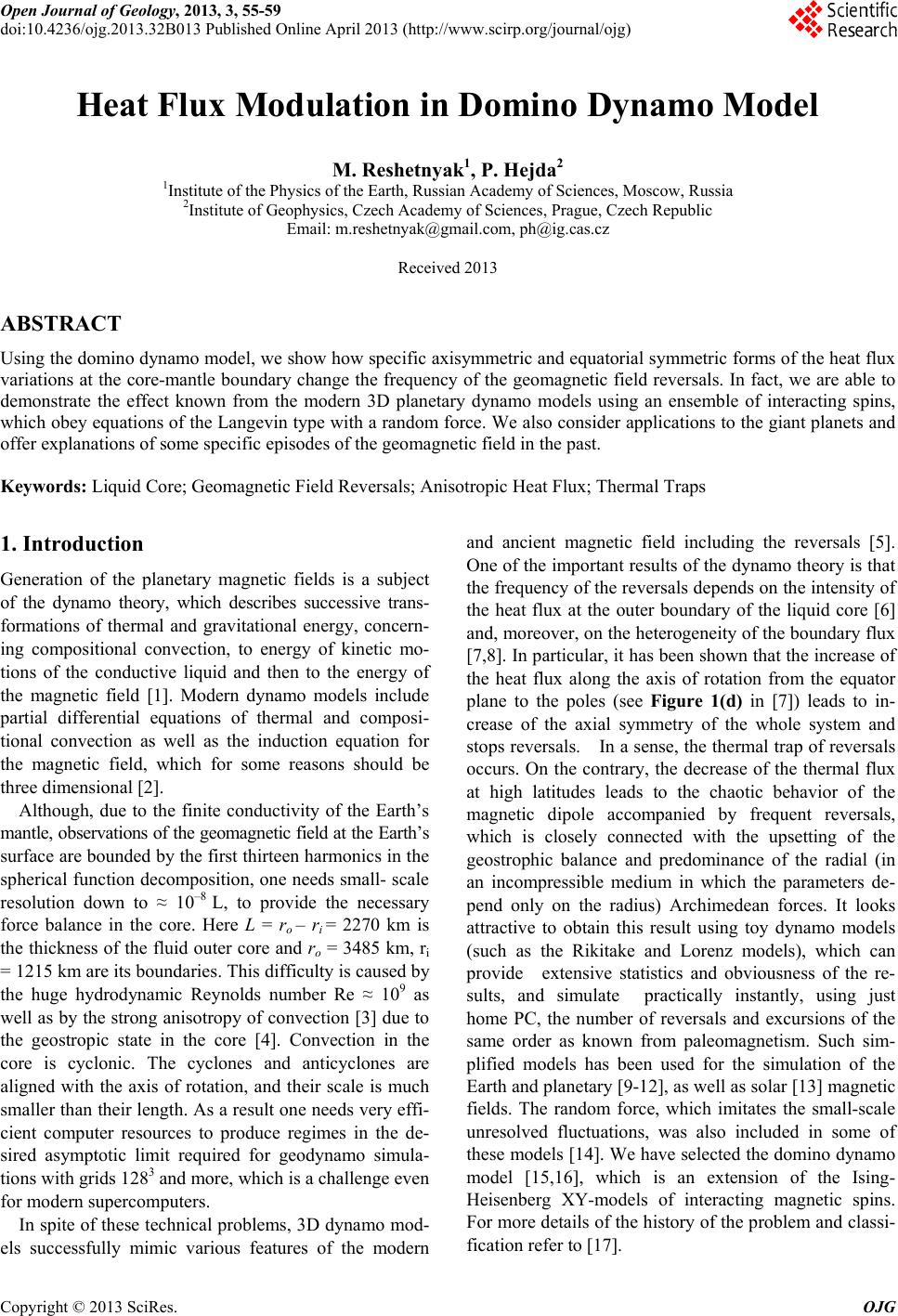
For negative C, when the geostrophy breaks due to
the relative intensification of convection in the equatorial
plane, we get the opposite result, see Figure 1(c): the
regime of the frequent reversals observed in Figure 1(c)
in [7]. In this case force F is directed from the poles and
the equilibrium point at the poles becomes unstable. The
new minimum of the potential energy at the equator leads
to the appearance of a new attractor, so that for C = -5
the axial dipole fluctuates with zero mean value and
maximal amplitude M~0.4. This state corresponds to the
equatorial dipole.
1
1
()sin( ()),
N
e
i
i
M
t
N


t (5)
so that |Me|~1 and does not undergo reversal. Similar
behavior of the magnetic dipole is observed on Neptune
and Uranus; for more details see, e.g. [21].
Now we consider ψ = -cos22
1
θ for which the corre-
sponding force F = -2sin4θ changes sign in each hemi-
sphere, see the example with the second-order zonal
spherical harmonic -, where is associated Leg-
endre polynomials, in Figure 1(e) in [7].
0
4
Pm
l
P
For C > 0, the potential barrier is in the middle lati-
tudes, which prohibits the reversals as observed in Fig-
ure 1(e) in [7]. In one of our runs only one reversal was
observed for C = 2. The other important point is the ex-
istence of the stable point at the equator, where M = 0.
We could then assume a regime with two attractors: near
the poles and at the equator. This regime is really ob-
served in Figure 1(d). The inverse transition was not
observed. Inspection of the state with small M at the be-
ginning of the run leads to a quite large estimate of the
equatorial dipole amplitude Me, see Figure 1(d). Thus, in
principle, this regime can also be related to the giant
planets’ dynamo as well.
The last example corresponds to the case C < 0, when
in addition to the attractors at the poles (related to rota-
tion ), two new attractors appear at the middle latitudes.
The variation of C leads to regimes C = -1 with fre-
quent reversals, observed in Figure 1(f) in [7]. Moreover,
we can get regimes, see Figrue 1(e), when the magnetic
pole stays at the high latitudes, however, ||M

(the
partial synchronization of the spins). There are some
jumps to the unstable state M = 0 with the dipole at the
equator. Note that the decrease of the spatial scale of 
leads to the increase of its amplitude C.
4. Conclusions
To conclude, let us stress that the toy models do not pre-
tend to compete with the known 3D dynamo models.
However, toy models are being developed for better un-
derstanding of physics of the processes. The main point
is that model of the spins does have a background based
on our present knowledge of the flow structure in the
core. The system of the cyclones in the core, which act
like the individual magnets, produces the net magnetic
flux observed outside the volume of generation. These
individual magnets can interact with each other, feel the
direction of angular rotation and are disturbed by the
thermal-compositional convection forces. The domino
model is based on the function decomposition related to
the geostrophic state. It is the geostrophy, which is re-
sponsible for the cyclone formation along the axis of
rotation.
REFERENCES
[1] G. Rudiger and R. Hollerbach, “The Magnetic Universe:
Geophysical and Astrophysical Dynamo Theory,”
Wiley-VCHr, Weinheim, 2004.
[2] C. A. Jones, “Planetary Magnetic Fields and Fluid Dy-
namos,” Annual Review of Fluid Mechanics, Vol. 43,
2011, pp. 583-614.
doi:10.1146/annurev-fluid-122109-160727
[3] P. Hejda and M. Reshetnyak, “Effects of Anisotropy in
the Geostrophic Turbulence,” Physics of the Earth and
Planetary Interiors, Vol. 177, 2009, pp.152-160.
doi:10.1016/j.pepi.2009.08.006
[4] J. Pedlosky, “Geophysical Fluid Dynamics,” Springer-
Verlag, New York, 1987.doi:10.1007/978-1-4612-4650-3
[5] U. R. Christensen, “Zonal Flow Driven by Strongly Su-
percritical Convection in Rotating Spherical Shells,”
Journal of Fluid Mechanics, Vol. 470, 2002, pp. 115-133.
doi:10.1017/S0022112002002008
[6] P. Driscoll and P. Olson, “Superchron Cycles Driven by
Variable Core Heat Flow,” Geophysical Research Letters,
Vol. 38, No. 9, 2011, p. L09304.
doi:10.1029/2011GL046808
[7] G. A. Glatzmaier, R. S. Coe, L. Hongre and P. H. Roberts,
“The Role of the Earth’s Mantle in Controlling the Fre-
quency of Geomagnetic Reversal,” Nature, Vol. 401,
1999, pp. 885-890. doi:10.1038/44776
[8] P. L. Olson, R. S. Coe, P. E. Driscoll, G. A. Glatzmaier
and P. H. Roberts, “Geodynamo Reversal Frequency and
Heterogeneous Core-Mantle Boundary Heat Flow,”
Physics of the Earth and Planetary Interiors, Vol. 180,
No. 1-2, 2010, pp.66-79. doi:10.1016/j.pepi.2010.02.010
[9] I. Melbourne, M. R. E. Proctor and A. M. Rucklidge, “A
Heteroclinic Model of Geodynamo Reversals and Excur-
sions,” Dynamo and Dynamics, a Mathematical Chal-
lenge, Kluwer, Dordrecht, Vol. 26, 2001, pp.
363-370.doi:10.1007/978-94-010-0788-7_43
[10] D. A. Ryan and G. R. Sarson, “Are Geomagnetic Rever-
sals Controlled by Turbulence within the Earth's core?”
Geophysical Research Letters, Vol. 34, 2007, p. L02307.
doi:10.1029/2006GL028291
[11] C. Narteau, J. L. Le Mouel, M. Shnirman, E. Blanter
and C. Allegre, “Reversal Sequence in a Multiple Scale

M. RESHETNYAK, P. HEJDA
59
Dynamo Mechanism,” Physics of the Earth and Plane-
tary Interiors, Vol. 120, No. 4, 2000, pp. 271-287.
doi:10.1016/S0031-9201(00)00145-X
[12] C. Narteau and J. L. Le Mouel, “Transient Evolution
Regimes in a Multiscale Dynamo Model: Timescales of
the Reversal Mechanism,” Journal of Geophysical Re-
search: Solid Earth, Vol. 110, 2005. p.B01104.
doi:10.1029/2004JB002983
[13] D. Volobuev, “Toy Dynamo to Describe the Long-Term
Solar Activity Cycles,” Solar Physics, Vol. 238, No. 2,
2006, pp. 421-430. doi:10.1007/s11207-006-0154-x
[14] P. Hoyng, “Helicity Fluctuations in Mean Field Theory:
An Explanation for the Variability of the Solar Cycle?”
Astronomy
﹠ Astrophysics, Vol. 272, 1993, pp. 321-339.
[15] N. Mori, D. Schmitt, J. Wicht, A. Ferriz-Mas, H. Mouri,
A. Nakamichi and M. Morikawa, “Domino Model for
Geomagnetic Field Reversals,” Physical Review E, Vol.
87, 2013, p. 012108. doi:10.1103/PhysRevE.87.012108
[16] A. Nakamichi, H. Mouri, D. Schmitt, A. Ferriz-Mas, J.
Wicht and M. Morikawa, “Coupled Spin Models for
Magnetic Variation of Planets and Stars,” Monthly No-
tices of the Royal Astronomical Society, Vol. 423, 2012,
pp. 2977-2990. doi:10.1111/j.1365-2966.2012.20862.x
[17] H. E. Stanley, “Introduction to Phase Transitions and
Critical Phenomena,” Oxford University Press, Oxford,
1987.
[18] J. S. Gee and D. V. Kent, “Source of Oceanic Magnetic
Anomalies and the Geomagnetic Polarity Reversals,” In
Treatise on Geophysics, Geomagnetism (ed. M. Kono),
Elsevier, Amsterdam, Vol. 5, 2009, pp. 455-508.
[19] N. Zhang and S. Zhong, “Heat Fluxes at the Earth's Sur-
face and Core-Mantle Boundary Since Pangea Formation
and Their Implications fo the geomagnetic superchrons,”
Earth and Planetary Science Letters, Vol. 306, No. 3-4,
2011, pp. 205-216. doi:10.1016/j.epsl.2011.04.001
[20] A. Abrajevitch and Rob Van der Voo, “Incompatible
Ediacaran paleomagnetic Directions Suggest an Equato-
rial Geomagnetic Dipole Hypothesis,” Earth Planetary
Science Letters, Vol. 293, 2010, pp. 164-170.
doi:10.1016/j.epsl.2010.02.038
[21] A. V. Shatsillo, A. N. Didenko and V. E. Pavlov, “Two
Competing Paleomagnetic Directions in the Late Vendian:
New Data for The SW Region of the Siberian Platform,”
Russian Journal of Earth Sciences, Vol. 7, No. 4, 2005, p.
ES4002. doi:10.2205/2004ES000169
[22] I. Cupal, P. Hejda and M. Reshetnyak, “Dynamo Model
with Thermal Convection and with the Free-Rotating In-
ner Core,” Planet. Space Science, Vol. 50, 2002, pp.
1117-1122. doi:10.1016/S0032-0633(02)00051-X