M. A. CARDENETE, F. SANCHO
280
librium state we can quickly write the reduced form
linking output with instruments as q = (I − A)−1x = Mx,
with M representing the multiplier matrix of the linear
economy. Because of the assumptions on A, the matrix
M is constant. Its entries are independent of the equilib-
rium state. Taking derivatives, it is quite simple now to
relate changes in output with external changes in instru-
ments
1
qx
IA Mx
2
(1)
Multipliers are given directly by the cells in matrix M,
i.e. ∂qj/∂xi = mji. All that is needed to compute (linear)
multipliers is the coefficients matrix A. Since this matrix
is readily available from official statistics, this explains
the popularity of linear models in policy oriented em-
pirical economics. Even more, linear models are so sim-
ple that we need not worry about prices. Prices, in fact,
can be seen to be completely independent from quantities
in linear interindustry models. Notice that if quantities
are not affected by prices, neither are multipliers. End of
the story, all needed multiplier information is contained
in matrix M. But we know that the actual story is bit
more complicated than that since, in general, prices and
quantities are mutually dependent.
3. Applied General Equilibrium Mul tip li ers
In a standard general equilibrium model the interactions
of supply and demand determine, at the same time, prices
and quantities. We use now a general equilibrium frame-
work to elucidate multipliers and compare them to their
linear counterpart. Endogenous variables include now n
output levels q and n prices p, that is, , so in
total we have 2n endogenous variables. Let us consider
again that the government decides how much to buy of
each of the n goods and services; the government’s de-
mand levels are denoted by the vector x representing
policy instruments. The structural function F represent-
ing the equilibrium state would now be of the type
,eqp
2
:nn n
RR
2
:
qn
which in turn can be split in two func-
tions n n
R
R and 2
:
nn n
R
qp
R determin-
ing quantities and prices, respectively. The complete
general equilibrium state is represented by (q, p) = F(q, p,
x), or using the fact that
FF, it can also be seen
as
,,
,,
p
q
pFqpx
qFqpx
(2)
We perform comparative statics on the equilibrium
state represented in Equation (2) considering an exoge-
nous change dx in the instruments x. We would obtain
qq qp qx
pq pp px
dqMdq Mdp Mdx
dpM dqM dpMdx
(3)
where we use, in Equation (3), the notational convention
,,
q
qq
Fqpxq
,
,,
q
qp
Fqpxp , and so
on. Solving for dp in the second expression in Equation
(3) and substituting the result in the first equation would
yield
1
1
1
qq qp qx
qqqp pppq px
qx
qq qppppq
qx qppppx
dqMdq Mdp Mdx
dq MIMMdq Mdx
Mdx
MMIM Mdq
MMIM Mdx
(4)
Solving now for dq in Equation (4) we finally obtain
1
1
1,,
qq qppppq
qx qppppx
dqIMMI MM
MIM Mqpxdx
M
(5)
where
,,qpxM
M
stands for the general quantity mul-
tiplier matrix1. We now proceed to relate the linear mul-
tiplier matrix in Equation (1) with the general multi-
plier matrix
,,xqpM derived in Equation (5).
Recall first that in linear models quantities and prices
are independently determined. Under this assumption the
partial derivative matrices Mpq and Mqp would be such
that Mpq = Mqp = 0 and then Equation (5) can be easily
verified to reduce to
1
qq qx
dqIMM dx
(6)
The simplified expression that appears in Equation (6)
is of course the differential version of the classical linear
multiplier expression picked up in Equation (1) above,
with Mqq = A and Mqxdx = Δx. The chains of interactions,
however, can be seen to be quite more complex in Equa-
tion (5) than in Equation (1), in accordance with the
higher complexity of nonlinear models vis-a-vis linear
ones.
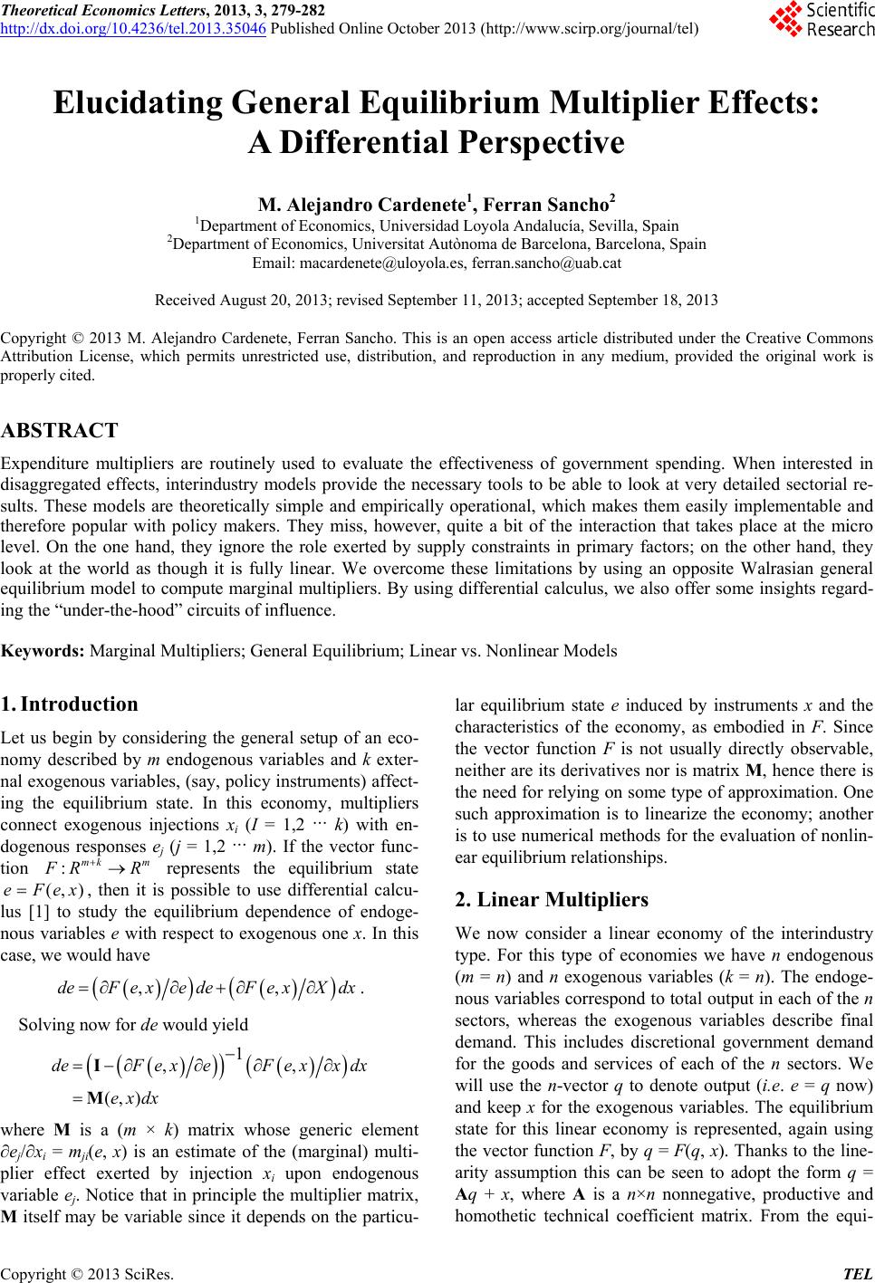
Figure 1 below depicts the way the model’s intercon-
nections work. Facing an external disturbance in x, the
system first reacts with changes in prices and quantities
through matrices Mpx and Mqx. Price effects repeatedly
self multiply through the loop Mpp along the cost struc-
ture which, in turn, are affected by cross effects Mqp from
quantities to prices. Similarly, the initial effect of the
disturbance on quantities gets itself multiplied by the
chain reaction that moves directly from quantities to
quantities, i.e. Mqq, and indirectly from quantities to
looped prices and back to quantities via the combined
1A similar derivation, that we omit, would produce a general price
multiplier matrix.
Copyright © 2013 SciRes. TEL