Journal of Modern Physics, 2013, 4, 1213-1380
http://dx.doi.org/10.4236/jmp.2013.410165 Published Online October 2013 (http://www.scirp.org/journal/jmp)
Stochastic Quantum Space Theory on Particle Physics
and Cosmology
—A New Version of Unified Field Theory
Zhi-Yuan Shen
Received May 14, 2013; revised June 14, 2013; accepted August 1, 2013
Copyright © 2013 Zhi-Yuan Shen. This is an open access article distributed under the Creative Commons Attribution License, which
permits unrestricted use, distribution, and reproduction in any medium, provided the original work is properly cited.
ABSTRACT
Stochastic Quantum Space (SQS) theory is a new version of unified field theory based on three fundamental postula-
tions: Gaussian Probability Postulation, Prime Numbers Postulation, Vacuon Postulation. It build a framework with
theoretical results agree with many experimental data well. Main conclusions of SQS theory are: 1) The 3-dimensional
Space with face-centered lattice structure attached to Gaussian probability is stochastic in nature. 2) SQS theory is
background independent at three levels. 3) Quarks with same flavor and different colors are different elementary parti-
cles. There are 18 quarks in three generations based on 18 prime numbers. 4) There are only three generations of ele-
mentary particles. 5) SQS theory elementary particles table listed 72 particles including 13 hypothetic bosons. Vacuon
is the only elementary particle at the deeper level. 6) Photon has dispersion and special relativity is revised accordingly.
7) Graviton has zero spin. 8) Entangled particles are connected by physics link with limited distance and non-infinite
superluminal speed. 9) All physical events are local, no “spooky action at a distance”. 10) Elementary particle is repre-
sented by discrete trajectories on geometrical model with genus number from 0 to 3. 11) Characteristic points and re-
lated triangles in elementary particle’s model provide its physics parameters. 12) Particles internal movements in a tra-
jectory are deterministic and uncertainty only comes from jumping trajectories. 13) Fermion’s mass exceeds
2
/973.4 cGeVMMax  must pair with anti-fermion serving as a boson state. 14) Fine structure constant is a running constant
2
)71/2(   based on a mathematic running constant

. 15) Converting rules based on Random Walk Theorem are
introduced to deal with hierarchy problems. 16) Logistic recurrent process and grand number phenomena play impor-
tant rules for converting factor in the transmission region between P
L71 and Compton length. 17) Based on
face-centered space structure, 36 symmetries )(rO , )(rC with P
Lr 3 are identified as the intrinsic symmetries serving
as the origin of all physics symmetries. 18) Heisenberg uncertainty principle is generalized with less uncertainty at
sub-Planck scale. 19) There are close correlations between elementary particle theory and three finite sporadic Lie
groups: M, B, Suz. 20) Cosmic structure and evolution are intrinsically correlated to elementary particles and prime
numbers. 21) A part of dark matters is 2-dimensional membranes left over from cosmic inflation driven by e-boson as
the inflaton. 22) After the big bang and before the current cosmic period, there are two cosmic periods with
3
1
1-dimensional space and 2-dimensional space. 23) A cyclic universe model is based on positive and negative prime
numbers. 24) A multiverse includes 22 10~ member universes organized in two levels. 25) The limited anthropic prin-
ciple is introduced. 26) A super-multiverse includes 44
10~ member multi-universes organized in two levels; Total
number of universes in the super-multiverse is 66 10~ . 27) Based on Poincare theorem, SQS theory introduces the ab-
solute black hole without any radiation. 28) A GUT including all four types of interactions occurs at 71 Planck lengths.
29) SQS theory primary basic equations are established based on Einstein equations for vacuum and redefined gauge
tensors attached to Gaussian probability. SQS Theory provides 25 predictions for experimental verification.
Keywords: Unified Field Theory; Space Structure; Elementary Particles; Gaussian Probability; Prime Numbers;
Sporadic Groups; GUT; Dark Matter; Dark Energy; Cosmos Inflaton; Multiverse; Anthropic Principle;
General Relativity; Primary Basic Equations

Z. Y. SHEN 1214
Section 1. Introduction
This paper is the continuation and extension of the au-
thor’s previous paper [1], which was published in Chi-
nese. For people not familiar with Chinese language, a
brief review of the previous paper is included in this paper.
Stochastic Quantum Space (SQS) theory initially was
intended to be a theory of space. It turns out as a unified
field theory including particle physics and cosmology.
In essence, SQS theory is a mathematic theory. Its re-
sults are interpreted into physics quantities by using three
basic physics constants, h, c, G or equivalently P
L,
P
t, )(PP ME . In principle no other physics inputs are
needed.
SQS theory is based on three fundamental postulations,
Gaussian Probability Postulation, Prime Numbers Postu-
lation, Vacuon Postulation, which serve as the first prin-
ciple of SQS theory.
Based on three fundamental postulations, SQS theory
builds a framework.
Based on Einstein’s general relativity equations for
vacuum and redefined gauge tensors attached to prob-
ability, SQS theory established the basic equations in-
cluding two parts. The microscopic part is the primary
basic equations for elementary particles, interactions and
things on upper levels. The macroscopic part as the av-
eraged version includes two sets of basic equations, one
set for gravity and the other set for electromagnetic force.
SQS theory provides twenty five predictions for veri-
fications.
The basic ideas of SQS theory are summarized as the
following:
1) Space is a continuum with grainy structure. It is
stochastic in nature represented by Gaussian probability
distribution functions at discrete points. Elementary par-
ticles and interactions are different types of movement
patterns of the space.
2) Cosmology and particle physics are intrinsically
correlated with mathematics, in which prime numbers
play the central role.
3) The correct way to unify general relativity theory
with quantum theory is to introduce probabilities to Ein-
stein’s original equations for vacuum.
SQS theory laid down the foundations and built a
framework. There are many open areas for physicists and
mathematicians to explore and contribute.
Section 2. Gaussian Probability Assignment
According to Stochastic Quantum Space (SQS) theory,
space is stochastic and continuous with grainy structure
in Planck scale.
The Planck length is:
35
31061625.1
2

c
hG
LP

m, (2.1a)
Based on P
L, Planck time P
t, Planck energy P E
and Planck mass P
M are defined as:
s
c
hG
c
L
tP
P44
51039123.5
2



, (2.1b)
J
G
hc
L
hc
E
P
P10
5
1022905.1
2

, (2.1c)
kg
G
hc
cL
h
M
P
P7
10367498.1
2


. (2.1d)
In which h, c and G are Planck constant, speed of
light in vacuum and Newtonian constant of gravitation,
respectively.
Postulation 2.1A. Gaussian probability postulation.
The relation between different points in space is stochas-
tic in nature. Gaussian probability distribution function is
assigned to each discrete point i x separated by Planck
length. In 1-dimensional case, the Gaussian probability at
point
x
is:


2
2
2
2
1
;


i
xx
iexxp


;







,,0,,x;








,,2,1,0,1,2,,
i
x. (2.2)
The distance between adjacent discrete points is nor-
malized to 1
P
L.
Explanation: The Gaussian Probability Postulation
serves as the first fundamental postulation of SQS theory.
It represents the stochastic nature of space and also
represents the quantum nature of space without sacrific-
ing space as a continuum. The

i
xxp ; serves as the
value at point
x
from the Gaussian probability distribu-
tion function centered at discrete point i x. Postulation
2.1 is for 1-dimensional case as the foundation for
3-dimensional case.
The Standard Deviation (SD)

of Gaussian prob-
ability is selected to let the numerical factor in front of
exponential term in (2.2) equal to 1:
014333989422804.0
2
1


. (2.3)
The reason of selecting such specific value for

will
be explained later.
Substituting (2.3) into (2.2) yields:



2
;i
xx
iexxp


;



 ,,0,,x;

 ,,2,1,0,1,2,,
i
x. (2.4)
Postulation 2.1B. In the 3-Dimensional Case, (2.2) is
Extended as


  
2
222
2
3
2
3
2
1
,,;,,


kji zzyyxx
kjiezyxzyxp


;

Z. Y. SHEN 1215




,,0,,,, zyx ;


 ,,2,1,0,1,2,,,, kji zyx . (2.5)
The values of

are determined by the roots of the
following equation:
01)2( 32/3  
. (2.6)
Equation (2.6) has three roots:


2
1
'0,



2
'
3/2
1
i
e
,



2
'
3/4
2
i
e
. (2.7)
Substituting
 2/1'0 into (2.5) yields:

   
222
,,;,, kji zzyyxx
kji ezyxzyxp 


;



 ,,0,,,,zyx ;


 ,,2,1,0,1,2,,,, kji zyx . (2.8)
In (2.8), only the real root of
 2/1'0 is used.
The meaning of all three roots will be discussed later.
Definition 2.1: The Gaussian sphere centered at
),,( kji zyx is defined as its surface represented by the fol-
lowing equation:
2222 )()()(Rzzyyxx kji  . (2.9a)
The radius of Gaussian sphere is defined as:
932743535533905.0
22
1R. (2.9b)
Explanation: The 3-dimensional Gaussian probability
distribution of (2.8) has spherical symmetry like a sphere
with blurred boundary. The Gaussian sphere is defined
with a definitive boundary. It plays an important role for
the structure of space as shown in Section 22.
For the 1-dimensional case, according to (2.4), the un-
itarity of probability distribution function ),( i
xxp with
respect to continuous variable
x
is satisfied for any dis-
crete point i
x:


1; 2  



 dxedxxxp xx
ii

. (2.10)
In general, the unitarity of probability ),( i
xxp with
respect to discrete variable i x is not satisfied.
Definition 2.2: S-Function. Define the summation of
),( i xxp with respect to i
x as the
 xS-function:
 








i
i
ix
xx
xiexxpxS 2
;

. (2.11)
Theorem 2.1: S-function

 xS satisfies periodic con-
dition:
 xSxS  1. (2.12)
Proof: According to (2.11):

 

)(1
2
22 )1(1 xSeeexS
j
j
i
i
i
i
x
xx
x
xx
x
xx  










.
QED
The values of

 xS in the region 10  x are listed
in Table 2.1 and shown in Fig. 2.1.
Table 2.1: The values of
 xS in region 10


x.
In the region

 1,0 , except two points at 25.0

x and
75.0

x, in general

 xS defined by (2.11) does not
satisfy unitarity requirement, which has important impli-
cations.
0.9
0. 92
0. 94
0. 96
0. 98
1
1. 02
1. 04
1. 06
1. 08
1.1
00.1 0.20.3 0.40.50.60.7 0.80.91
x
S(x)
Figure 2.1.

 xS curve in region 10

x.
Theorem 2.2:

 xS satisfies the following symmet-
rical condition:



 xSxS


1, 10 x. (2.13)
Proof: According to (2.11):




)(1
2
22 )1(1 xSeeexS
j
j
i
i
i
i
x
xx
x
xx
x
xx   










. QED
Def inition 2.3: S

-Function. Define the S

- func-
tion as:

 1)( 


xSxS . (2.14)
Numerical calculation found that
 xS satisfies the
following approximately anti-symmetrical condition:



 xSxS





5.0 , 5.00 x. (2.15)
The symmetry of

 xS with respect to 5.0

x in
region

 1,0 given by (2.13) is exact. The anti-symmetry
of

 xS

with respect to 25.0x in region

 5.0,0
given by (2.15) is approximate with a deviation less
than 5
10. The deviation is tiny, but its impact is signifi-
cant. It plays a pivotal role for SQS theory, which will be
shown later.

Z. Y. SHEN 1216
Numerical calculation found that at the center 25.0

x
of the region
 5.0,0 :
 152889999930253.025.0 S. (2.16)
(2.16) indicates that,
 25.0S has a deviation of
6
107~   from 1 required by the unitarity. Numerical
calculation found a point c
xin region [0, 0.5] satisfying
unitarity:
 1
c
xS, (2.17)

 
5.0
0
0)(11)(
c
c
x
x
dxxSdxxS , (2.18)
73026452499871562.0
c
x. (2,19)
On the x-axis, c
xis located at the left side of
25.0x. It extends the region of
 1xS and shrinks
the region of
 1xS . The special point c
x has a pro-
found effect on elementary particles and unifications of
interactions, which will be given in later sections.
Definition 2.4: Based on c
x, three other special points
a
x,b
x,d x are defined:
3726973550.250012845.0  cd xx . (2.20)
   
 
25.0
0
011
c
a
x
x
dxxSdxxS .
10
10882111819946879.5  
a
x. (2.21)
   
 
25.0
0
0
c
b
x
x
dxxSdxxS ,
-5
10918477191.18218617 
b
x. (2.22)
The physics meaning of four special points, a
x, b
x,
c
x, d x, will be given later.
In 3-dimensional case, according to (2.8), the unitarity
of


kjizyxzyxp ,,;,, with respect to continuous vari-
ables x, y, z is satisfied for any discrete point


kji zyx,, :

   
.1
,,;,,
2
2
2
222
)(
)(
)( 

























dzedyedxe
edzdydxzyxzyxdzpdydx
k
j
i
kji
zz
yy
xx
zzyyxx
kji

(2.23)
In general, the unitarity of probability


kji zyxzyxp ,,;,,
with respect to discrete variables kji zyx ,, is not satis-
fied.
Definition 2.5: Define the summation of the probabil-
ity


kjizyxzyxp,,;,, with respect to kji zyx ,, as:
 
   
 













ijk
kji
ijkxyz
zzyyxx
xyz kji ezyxzyxpzyxS 222
,,;,,,,
3

.
(2.24)
Theorem 2.3:


zyxS,,
3 can be factorized into three
factors:






).()()(
,,
2
2
2
222
)(
)(
)(
3
zSySxSeee
ezyxS
k
k
j
j
i
i
ijk
kji
z
zz
y
yy
x
xx
xyz
zzyyxx










































(2.25)
Proof: The three-fold summation in (2.25) includes
terms for all possible combinations of 2
)( i xx
e , 2
)( j yy
e ,
2
)( k zz
e . The three multiplications in (2.25) include the
same terms. They are only different in processing, the
results are the same. QED
By its definition and (2.12), (2.25),
 zyxS,,
3 satisfies
the following periodic conditions:

 
zyxSzyxS,,,,1 33


, (2.26a)

  zyxSzyxS,,,1, 33


, (2.26b)

  zyxSzyxS ,,1,, 33  . (2.26c)
Definition 2.6: Planck cube is defined as a cube with
edge lengths 1
P
L and with discrete point ),,( kji zyx at
its center or its corner.
The values of

 zyxS,,
3 at 125 points in a Planck
cube with discrete points at its corner are calculated from
(2.24) and listed in Table 2.2.
Table 2.2.

 zyxS ,,
3 values at 125 points in a Planck cu-
be (Truncated at

1000).
Theorem 2.4: Probability Conservation Theorem.
The average value of

 zyxS,,
3 over a Planck cube
equals to unity:
  1,,,, 3
1
0
1
0
1
0
3

zyxSdzdydxdvzyxS
PlanckCube
. (2.27)
Proof: Substitute (2.24) into left side of (2.27):
 






























ijk
kji
ijk
kji
xyz
zzyyxx
xyz
zzyyxx
PlanckCube
edzdydx
edzdydx
zyxSdzdydxdvzyxS
1
0
1
0
])()()[(
1
0
])()()[(
1
0
1
0
1
0
3
1
0
1
0
1
0
3
.
,,,,
222
222


(2.28)
Change variables as:

Z. Y. SHEN 1217
,'xxx i ,' yyy j zzz k'. (2.29)
Substituting (2.29) into (2.28) and changing integra-
tions’ upper and lower limits accordingly yield:
 


.1'''
'''
,,,,
222
222
)'()'()'(
11
)'()'()'(
1
3
1
0
1
0
1
0
3





















kji
ijk
i
i
j
j
kji
k
k
zzyyxx
xyz
x
x
y
y
zzyyxx
z
z
V
edzdydx
edzdydx
zyxSdzdydxdvzyxS


QED
Probability Conservation Theorem is important. It
proved that, even though in general
 zyxS ,,
3 does not
satisfy unitarity requirement, but it does satisfy unitarity
requirement in terms of average over a Planck cube. The
conservation of probability means that, the event carriers
of probability are moving around but they cannot be cre-
ated or annihilated.
Lemma 2.4.1: The average value of
 xS over re-
gion [0,1] equals to unity:


1
0
1dxxS . (2.30)
Proof: Substitute (2.11) into the left side of (2.30):


 




 
i
i
i
i
x
xx
x
xxedxedxxS
1
0
)(
1
0
1
0
2
2
 . (2.31)
Change variables as:
xxx i'. (2.32)
Substituting (2.32) into (2.31) and changing integra-
tion’s upper and lower limits accordingly yield:


 



 
 1' 22 '
1
'
1
0
dxedxedxxS x
x
x
x
x
i
i
i

. QED
Lemma 2.4.2: Planck cube with volume 1

V (leng-
th normalized to 1
P
L) is divided into two parts 1 V
and 2
V:
1
21  VVV , (2.33a)
,1

V
Vdv ,
1
1

V
Vdv .
2
2

V
Vdv (2.33b)
Theorem 2.4 leads to the following equation:
  




12
,,11,, 33
VV
dvzyxSdvzyxS. (2.34)
Proof: According to (2.27) and (2.33):
 


212112
21333 1),,(,,,,
VVVVVV
d
v
dvVVVdvzyxSdvzyxSdvzyxS.
Moving the terms on left and right sides yields (2.34).
QED
Section 3. Unitarity
Unitarity is a basic requirement of probability. As shown
in Section 2, the unitarity with respect to discrete vari-
ables and continuous variables for Gaussian probability
are contradictory. In this section, three schemes are pre-
sented to solve the unitarity problem.
Scheme-1. To Treat All Points in Space Equally
For Scheme-1, Gaussian probabilities are not only as-
signed to discrete points but to every point in the con-
tinuous space. The summations in
 zyxS ,,
3 of (2.24)
introduced in Section 2 become integrations:
  
 
 .1'''
'''',',';,,,,;,,,,
'')'(
3
2 2
























zSySxSdzedyedxe
dzdydxzyxzyxpzyxzyxpzyxS
zzyyxx
xyz kji
ijk

(3.1)
The unitarity problem is solved.
For Scheme-1, the discrete points are no longer special
and all points in the space are on an equal footing. But
Scheme-1 does not represent the space for SQS theory,
instead, it represents the space for quantum mechanics.
To introduce Scheme-1 is for comparison purpose. It
indicates that, the uniform space does not have unitarity
problem. The unitarity problem is caused by space grainy
structure, which SQS theory must deal with.
Let’s go back to the grainy space proposed by SQS
theory. In Appendix 1, A Fourier transform is applied to
probability


xp of (2.4) to convert it into k-space. Ac-
cording to (A1.2), the corresponding Gaussian probabil-
ity function

 kP in k-space is:



4
2
2
1k
ekP   . (3.2)
The standard deviation of


kP is .2  
k Mul-
tiplying (A1.6) with yields:

   xpxk 
. (3.3)
In (3.3), x

and x
pare 1-dimensional displacement
and momentum difference, respectively. The  on right
side is two times greater than the minimum value 2/
from Heisenberg uncertainty principle. The increased
uncertainty is due to the asymmetry of
 2/1 and
 2
k.
The wave function corresponding to

i
xkP ; of (A1.1)
is:

i
ikx
k
iieexkQkPxk



8
2
2
1
);()(;

 ;




,,0,, k;



,,2,1,0,1,2,, 
i
x. (3.4)
Notice that, the wave function (3.4) has following fea-
tures:
1) The relation between

i
xkP ; and

i
xk;

is con-

Z. Y. SHEN 1218
sistent with quantum mechanics:
 
iii xkxkxkP;;;


. (3.5)
2) Only discrete points i
x appear in the phase func-
tion i
ikx
e.
3).

i
xk;

is not an eigenstate of k. The magni-
tude )(kP of

i
xk;

serves as distribution function
for k.
Before explore other schemes, a discussion for the es-
sence of probability unitarity is necessary. Probability is
associated with events. In Section 2, Table 2.2 data show
that, in the vicinity of Planck cube’s center


5.0,5.0,5.0 zyx ,
the sum of probabilities
 1,,
3zyxS. Because the set of
events at these points are incomplete; some events are
missing. These missing evens cause the sum of local
probabilities less than one. In the vicinity of the Planck
cube corners


kji zyx ,, ,
 1,,
3zyxS , because the set
of events over there includes some events belong to other
places. These excessive evens cause the sum of local
probabilities greater than one. In other words, events
associated with their probabilities move around inside
Planck cube causing the unitarity problem. To move
these events back to where they belong will solve the
discrete unitarity problem. But it distorts the Gaussian
probability distribution and jeopardizes the unitarity with
respect to continuous variables based on Gaussian prob-
ability distribution.
To solve the problem requires some new concept. Tra-
ditionally, unitarity is local, which requires the sum of
probability equals to unity at each point in space.
 1,,
3zyxS is caused by events moving around. The
foundation for local unitarity no longer exists. A gener-
alized unitarity is proposed:
1) Recognize the fact that events associated with
probabilities move around;
2) Follow the moving events for probability unitar-
ity.According to Theorem 2.4, the Probability Conserva-
tion Theorem, generalized unitarity is not contradictory
to the traditional unitarity for the Planck cube as a whole
entity. But it does change the rules inside the Planck cube.
For the microscopic scales, as the events inside Planck
cube are concerned, generalized unitarity is necessary.
For the macroscopic scale including many Planck cubes,
the local unitarity is still valid in the average sense.
The following two schemes are based on generalized
unitarity.
Scheme-2. Unitarity via Probability
Transportation on Complex Planes
The complex planes are inherited from the
3-dimensional Gaussian probability. Consider a Planck
cube centered at a discrete point )0,0,0(

 kji zyx as
shown in Figure 3.1. According to (2.5), the
3-dimensional Gaussian probability is:


2
222
2
3
2
3
2
1
0,0,0;,,


zyx
ezyxp


. (3.6)
Normalize the three values of the standard deviations
0
'

,1
'

, 2
'

of (2.7) as:
1'200  
,
3/2
11 '2


i
e ,
3/2
22 '2


i
e . (3.7)
In which two of them 1

and 2

are complex num-
bers. To keep the probabilities as real numbers related to
1

and 2

, it is necessary to extend the x-axis, y-axis,
z-axis into three complex plans x -plane, y
-plane, z
-
plane, respectively.
Figure 3.1. The Planck cube with center at a discrete point
)0,0,0(



kji zyx.
Definition 3.1: Define parameters to build three com-
plex planes associated with x-axis , y-axis, z-axis:

 
 i
exx  2,12,1
, (3.8a)

 

 i
eyy   2,12,1
, (3.8b)

  
i
ezz   2,12,1
, (3.8c)

120
3
2


.
(3.8d)
In which



,, and



,, are real parameters.
Explanation: In (3.8a), 2,1

 represents two straight
lines on complex x -plane intercepting to the real x-axis
at


x
with angles of 
120 
. Continuously

Z. Y. SHEN 1219
change the value of

, 1

 and 2

 sweep across x-axis
to construct the complex x
-plane. Every point on the
complex x
-plane is the intersection of two straight lines
defined by (3.8a). They
-plane and z -plane associated
with y-axis and z-axis are constructed in the same way.
On the complex x
-plane, three straight lines 1

, 2


and x-axis intercept at 0



x with 3-fold rotational
symmetry as shown in Figure 3.2. The 3-fold rotational
symmetry has its physics significance, which will be
discussed later.
Figure 3.2. Three straight lines with 3-fold rotational sym-
metry on complex x
-plane.
Rule 3.1: In order to keep the values of


i
xxp ;,


kji zyxzyxp ,
,;,, and


xS ,
 zyxS ,,
3as real numbers,
in the Gaussian probability exponential part, spatial va-
riables
x
y
x
,, in the numerator choice their path ac-
cording to (3.8) matching the

value in denominator
to keep these values always equal to real numbers.
Explanation: The validity of Rule 3.1 to


i
xxp;,


kji zyxzyxp ,
,;,, is obvious. Its validity for

 xS ,
 zyxS ,,
3 needs explanation. According to the definition
of


xS :


 





i
i
ix
xx
xiexxpxS2
;

. (2.11)
All terms of
 




i
xi
xxpxS ; except

0;xp have
their “tail” in region ]5.0,5.0[ , which are equivalent to
the “tails” of


0;xp in regions of ]5.0,[

 and
],5.0[  :

 

 


 




x
x
x
x
x
x
xx etoequivalente
i
i
i
5.0
,5.0
)0(
5.05.0
;0
)( 2
2
 
. (3.9)


xS in region [−0.5,0.5] can be viewed as a single
probability distribution function
 0;xp with “mul-
ti-reflections” at the two boundaries of region [−0.5,0.5].
Figure 3.3 shows an example for the 0
i
x term along
with two adjacent terms 1
i
x and 1
i
x with their
“tails” in region [−0.5,0.5]. In essence, probability trans-
portation via complex plane for

i
xxp ; is also valid for

 xS . According to Theorem 2.3,


)()()(,,
3xSySxSzyxS ,
the same argument is valid for
 zyxS,,
3 as well.
Figure 3.3. Three adjacent Gaussian probability distribu-
tion functions show the “tails”.
For double check, let’s look it the other way, consider
the


i
xxp; term in


xS :

2
2
)(
;


i
xx
iexxp


. (3.10)
In which i x is a real number and
x
is a complex
number. As long as the point corresponding to


i
xx is
on the lines defined by (3.8a),

i
xxp; is a real number,
and so is

 xS ..
In the Planck cube centered at discrete point
)0,0,0(  kji zyx as shown in Fig. 3.1, a closed sur-
face S is defined by




01,,
3zyxS , which divides
Planck cube in two parts 1
V and 2 V. In the inner region
1
V,



 01,, 1
3

V
zyxS ; in the outer region 2
V,



 01,, 2
3 V
zyxS. By means of probability transportation,
the excessive events associated with probabilities in the
inner region 1
V transport to the outer region 2 V. Ac-
cording to Theorem 2.4 and lemma 2.4.2,


zyxS ,,
3
satisfies generalized unitarity.
Since



 zSySxSzyxS

1113,, and

 xS ,

 yS ,

 zS have the same type of exponential expression, ex-
ploring one,

 xS , is sufficient. (2.13) shows that, in
region [0,1],


xS is symmetry with respect to5.0

x,
to explore

 xS in the half region [0,0.5] is sufficient. In
region [0,0.5], (2.15) shows that
 1)(

 xSxS is
approximately anti-symmetry with respect to 25.0

x.
In the meantime, let’s treat it as exactly anti-symmetry
and consider the difference later.
In Scheme-2, probabilities along with events transport
back and forth to satisfy the discrete and continuous uni-
tarity requirements alternatively.
Fermions and bosons are essentially different particles
with different properties. Their probability transporta-
tions are different. It turns out that, bosons without mass

Z. Y. SHEN 1220
take the straight real path along the real axis; while Dirac
type fermions take the zigzagging path on the complex
plane.
The following rules of probability transportation are
for Dirac type fermions.
Rule 3.2: The probability transportation rules for fer-
mions are as follows.
1) Consider two points

 25.00, 11 xx , 12 5.0xx


)5.025.0( 2 x along the real x-axis, as shown in Fig.
3.4. The excessive probability
 1
1xS at 1
x trans-
ports along a set of complex lines 1

 and 2

 to 2
x
where probability having deficient
 1
2xS. The path
length is:

12
2xxl  . (3.11)
The factor 2 in (3.11) comes from:
  2120cos/1cos/1  
. (3.12)
The probability transportation makes

1
1

xS and
 1
2xS to satisfy unitarity with respect to discrete va-
riable i x. But it distorts the Gaussian probability with
respect to continuous variable
x
.
Figure 3.4. Transporting paths with the same loop lengths
and different routs on complex plane.
2) To reinstall the Gaussian probability distribution, it
transports back from 2
x to 1 xalong another set of
complex lines 1

 and 2


via another path with the
same path length

12
2xxl as shown in Fig. 3.4.
The two paths form a closed loop with loop length:

12
42 xxlL  . (3.13)
The probability following its event goes back and forth
between 1
x and 2 x around closed loops.
3) The path length of (3.11) and the loop length of
(3.13) are valid for all zigzagging paths shown in Fig.3.4.
The multi-path nature has its physics significance, which
will be discussed in later sections
The repetitive probability transportations along closed
loops cause oscillating between two points 1 x and 2
x.
In this way, the two types of local unitarity are satisfied
alternatively, and the generalized unitarity is always sat-
isfied. It provides a kinematic scenario for the oscillation.
The dynamic mechanism and driving force of the oscilla-
tion will be discussed in Scheme-3.
As mentioned in Section 2, the anti-symmetry of



 xSxS





5.0 is only an approximation. In gen-
eral, the unitarity by probability transportation is not ex-
act. The tiny difference between 
1
xS and




2
xS
provides a slight chance for probability transportation
path to go off loop. The off loop path goes to other places
with different values of 1
x and 2 x corresponding to
other particles, which provide the mechanism for interac-
tions between particles and transformation of particles.
This is the scenario of probability transportation on the
complex x
-plan associated with x-axis. The same is for
the complex y
-plane and
z
-plane associated with
y-axis and z-axis.
For Scheme-2, the three real axes in 3-dimensional
real space are extended to three complex planes with 6
independent variables instead of 3. The extended space
with three complex planes is an abstract space. For SQS
theory, the real space is 3-dimensional. The essence of
complex plane is to add the phase angle to real spatial
parameters. The physics meaning of the phase angle will
be discussed later.
Scheme 3. Unitarity in Curved 3-Dimensional
Space
According to general relativity, in 3-dimensional
curved space, the distance between point ),,( zyxP and
discrete point ),,( kjid zyxP is the geodesic length:




kjiGdG zyxzyxLPPL ,,;,,;

. (3.14)
According to (A2.2) in Appendix 2, geodesic length


dGppL ; is determined by following differential equa-
tion:
.,0
2
2
d
cb
a
bc
aPtoP
ds
dx
ds
dx
ds
xd (3.15)
In which, ab
g is the gauge tensor and a
bc
 is Chris-
toffel symbol of second type. Taking

dG PPL ;
2 to re-
place


222 )()()( kji zzyyxx  in (2.24) yields:











ijk
kjidG
xyz
zyxPzyxPL
ePS ),,();,,(
3
2

. (3.16)
As mentioned previously, at point ),,( 1111 zyxP in 1
V
shown in Fig. 3.1, there are excessive events associated
with

 01)( 1
13

V
PS; at point ),,( 2222zyxP in 2
V, there

Z. Y. SHEN 1221
are deficient events associated with
 01)( 2
23

V PS . For
scheme-3, the probability transportation from 1
P to 2 P
takes its geodesic path:
 
),,();,,(, 22221111212121 zyxPzyxPLPPL . (3.17)
To adjust gauge tensor
 zyxgab,, along the path

2121 ,PPL in curved space, the unitarity of probability
 01)(1
13V
PS at 1
P and
 01)( 2
23  V
PS at 2
P are satis-
fied. But the Gaussian probability is distorted. Then the
gained probability at2
P transports back to1 P takes the
geodesic path:
  ),,();,,(, 11112222121212 zyxPzyxPLPPL. (3.18)
It goes back to1
P to reinstall Gaussian probability.
The transportations via


2121 ,PPL and

1212 ,PPL  fin-
ish one cycle of oscillation. The process goes on and on.
In this way, the local unitarity requirement with respect
to discrete variables and continuous variables of Gaus-
sian probability are satisfied alternatively, and the gener-
alized unitarity is always satisfied. This is the scenario of
probability oscillation in 3-dimesional curved space.
Hypothesis 3.1: To adjust the gauge tensor
 zyxgab,, properly makes geodesic paths


2121 ,PPL
such that
 01)(1
13 V
PS and

 01)( 2
23  V
PS are satis-
fied. To adjust the gauge tensor
 zyxgab,, properly
makes geodesic paths

1212 ,PPL  such that the Gaussian
probability is reinstalled. The adjusted
 zyxgab ,, de-
termines the space curvature inside the Planck cube.
Explanation: According to Hypothesis 3.1, the alter-
native unitarity of Gaussian probability with respect to
discrete variables and continuous variables is not only
the driving force for probability oscillation, but also
serves as the driving force to build the curved space in-
side Planck cube. This is the expectation from SQS the-
ory.
Let’ go back to the 1-dimension case.
Definition 3.2: S-equatio n. Define the S-equation
along the x-axis as:
011)( 2
)(  



i
i
x
xx
exS

. (3.19)
Explanation: S-equation is the origin of a set of sec-
ondary S-equations serving as the backbone of SQS the-
ory. It plays a central role to determine particles parame-
ters on their models, which will be discussed in later sec-
tions.
Theorem 3.1: Along the x-axis, the 1-dimensional un-
itarity requires:
011)( 2
))(( 



i
i
x
xxx
exS

for all
x
. (3.20)
The only way to satisfy01)( xS for all
x
is that
)(x


 is a function of
x
as a running constant.
Proof: In Section 2, (2.17) show that,
1)73026452499871562.0()( 

SxSc.
For allother points in region [1,0.5],
 1 c xxS . In
order to satisfy


01


xS for all x, something in the


xS must be adjustable. There are only two constants
e and

in

 xS. In which e as a mathematical
constant does not depend on geometry, while

does.
Therefore, the only way to satisfy unitarity of

 1

xS
for all x is that )(x



is a function of
x
as a run-
ning constant. QED
Explanation: For SQS theory, Theorem 3.1 plays a
central role for the models and parameters of elementary
particles, which will be demonstrated in later sections.
In the 1-dimensional case, what does

 x

mean?
The answer is:

 x

carrying information in curved
3-dimensional space around point
x
,




x indi-
cates space having positive curvature corresponding to
attraction force;




x indicates space having nega-
tive curvature corresponding to repulsive force. The real
examples will be given later.
In Table 3.1, the values of
 x

calculated from
(3.20) are listed along with the types of space curvatures
and corresponding forces.
Table 3.1.

 x

as a function of
x
calculated from (3.20)
(i
x truncated at 1000000

).
Notes: *The precision of values for


5
102.1 x 
is limited by 16-
digit numerical calculation. The lower limits are listed.
The attraction force is the ordinary gravitational force.
The repulsive force means that, in the vicinity of discrete
point gravity reverses its direction. This is one of predic-
tions provided by SQS theory, which is important in
many senses. For one, the repulsive force prevents form-
ing singularity, which solves a serious problem for gen-
eral relativity. For another, without repulsive force to
balance the attraction force, space cannot be stable. The
others will be given later.
Theorem 3.2: At discrete points i
xx , the unitarity
equation of (3.20) requires:



i
x 
, for





,,2,1,0,1,2,,
i
x. (3.21)

Z. Y. SHEN 1222
Proof: Consider the opposite. If

i
x 
is not infinity,
When the summation index 
i
x,



 
i
ii
x
xxx
iexS 2
))((
)(

.
Equation (3.20) cannot be satisfied. The opposite, i.e.
 
i
x 
must be true. QED
Theorem 3.2 is a mathematic theorem with physics
significance, which will be presented later.
For Scheme-2, probability oscillation is to satisfy al-
ternative unitarity, which does not provide the dynamic
mechanism and the driving force. For scheme-3, the re-
pulsive and attraction forces provide the dynamic me-
chanism and the driving force for oscillation. At 1
xx

where 1)( 1x

, the repulsive force pushes the event
associated with its probability towards 2
x. When it ar-
rived 2
xx  where 1)(2x

, the attractive force pulls
it back to 1
x. In this way, the oscillation continues. The
dynamic scenario provides the mechanism of oscillation,
which is originated from space curvature.
As mentioned in Scheme-2, the approximation nature
of anti-symmetry of (2.15) provides a slight chance for
transportation off loop representing interactions, which is
also valid for Scheme-3.
For Scheme-3, the curvature patterns make the Planck
scale grainy structure.
As a summary, Table 3.2 shows a brief comparison of
three schemes.
Table 3.2. Summary of the features for three schemes.
The three schemes are three manifestos of the vacuum
state. Scheme-1 corresponds to the quantum mechanics
vacuum state. Schemes-2 and Scheme-3 are SQS vacuum
states at a level deeper than quantum mechanics.
The probability oscillation in Scheme-2 is the same as
in Scheme-3. It implies that Scheme-2 is equivalent to
Scheme-3. Moreover, in Scheme-2, three complex planes
have 6 independent real variables; in Scheme-3, the
symmetrical 33 gauge matrix of ab
g also has 6 in-
dependent components. The correlation indicates that,
the complex planes of Scheme-2 are closely linked to
curved space of Scheme-3. It confirms that, the three
complex planes associated with three real axes are some
type of abstract expression of the curved 3-dimensional
real space. For SQS theory, there is no additional dimen-
sion or dimensions beyond the real 3-dimensional space
in existence.
In reference [2], Penrose demonstrated the correlation
between Riemann surface and the topological mani-
fold—torus. According to Penrose, 0

, 1

, 2

of (3.7)
are three branch points of the complex function 2/13 )1( z
on the Riemann surface:
1
0
 z, 3
2
1


i
ez ,3
4
2
2


i
ez  .
(3.22)
As shown in Figure 3.5(a), The Riemann surface for
2/13 )1( z has branch points of order 2 at 1,

, 2

and another one at

. Penrose showed that, for Rie-
mann surface’s two sheets each with two glued slits, one
from 1 to

and the other from

to 2

, these are
two topological cylindrical surfaces glued correspond-
ingly giving a torus as shown in Figure 3.5(b). On the
torus surface, there are four tiny holes 1
h, 
h,

h, 2

h
representing 1,

,

, 2

on the Riemann surface,
respectively. The four tiny holes on torus have important
physics significance, which well be discussed in later
sections.
Figure 3.5. (a): Four branch points and two glued cuts on
two sheets of Riemann surface; (b): Four tiny holes on torus
surface.
For SQS theory, the correspondence of Riemann sur-
face and torus is very important. It plays a pivotal rule
for constructing the topological models for quarks, lep-
tons, and bosons with mass and much more, which will
be discussed in later sections.
Section 4. Random Walk Theorem and
Converting Rules
Random walk process is based on stochastic nature of
space. It plays an important role for SQS theory. In this
section, the Random Walk Theorem is proved and con-
verting rules are introduced serving as the key to solve
many hierarchy problems.

Z. Y. SHEN 1223
Definition 4.1: Short Path and Long Path.
In 3-dimensional space, there are two types of paths
between two discrete points. The “short path”
L
from
point ),,( kji zyx to point ),,( '''kji zyx is defined as the
straight distance between them.
  
2
'
2
'
2
'kkjjiizzyyxxL . (4.1a)
The “long path”
L
ˆ from point ),,( kji zyx to point
),,( ''' kji zyx is defined as step-by-step zigzagging path in
lattice space with Planck length P
L as step length
Pi Ll.
P
N
iiNLlL  1
ˆ, nmlN 

. (4.1b)
The random walk from point ),,( kji zyx to point
),,( '''kjizyx takes l, m, n steps along
x
,
y

, z

directions, respectively.
Theorem 4.1: Random Walk Theorem. Short path
L
and long path L
ˆ are correlated by the random walk
formula:
2
ˆ
L
L
; or LL ˆ
. (4.2)
L
andL
ˆ are normalized with respect to Planck
lengt P
L, both are numbers.
Proof: According to (2.8), the probability from point
),,( kjizyx to point ),,('''kji zyx is:

   
2
2
'
2
'
2
'
''',,;,, L
zzyyxx
kjikji eezyxzyxp kkjjii



 . (4.3)
Take a random walk from


kji zyx ,, to


''' ,,kjizyx
with l, m, nsteps along
x

, y, z directions,
respectively. The probability of reaching the destination
is:


 L
lmn
nml
kjikji eeeeezyxzyxp ˆ
111
'''
222
,,;,,
  
nmlL 
ˆ. (4.4)
Combining (4.3) and (4.4) yields 2
ˆ
L
L
. QED
Obviously, Random Walk Theorem is based on Gaus-
sian Probability Postulation introduced in Section 2. As a
precondition, the standard deviation

of
3-dimensional Gaussian probability must take the values
to make the factor in front of exponential term equal to 1.
Otherwise, Random Walk Theorem does not hold. It
means that, the only parameter

in the first fundamen-
tal postulation of SQS theory is determined.
Random Walk Theorem provides the foundation for
conversions, which are governed by a set of converting
rules. Physics quantities can be converted by applying
these converting rules, which serve as the way to dealing
with hierarchy problems.
Definition 4.2: The converting factor for short path
and long path is defined as:
P
LLN /. (4.5)
Lemma 4.1:
L
, L
ˆ and
N
are related as:
P
LNNLL 2
ˆ . (4.6)
Proof: According to Theorem 4.1, the lengths
L
and
L
ˆ in (4.2) are normalized with respect to P
L. Let P L
appears in (4.2):
PPPPPL
L
N
L
L
L
L
L
L
L
L


















2
ˆ. (4.7)
Multiplying P
L to both sides of (4.7) yields:
NLL
ˆ. (4.8a)
According to (4.5), substituting P
NLL  into (4.8a)
yields:
P
LNL 2
ˆ. (4.8b)
(4.8a) plus (4.8b) is (4.6). QED
The basic unit of length in Theorem 4.1 and Lemma
4.1 as well as the step length of random walk is P
L,
which indicate the importance of Planck length.
According to SQS theory, physics quantities at differ-
ent scales have different values determined by converting
factors, which are governed by converting rules origi-
nated from Random Walk Theorem.
Definition 4.3: The conversion factors for general
purpose are defined as follows.
1) For bosons without mass:
P
LN /


. (4.9)

is the wavelength of the boson.
2) For particle s with mass:
PC LN/
 . (4.10)
C

is the Compton wavelength of the particle:
M
c
h
C

. (4.11)
M
is the mass of that particle and c is the speed of
light in vacuum.
Conversion rules for general purpose are given as fol-
lows.
1) For length:
P
LNNLL2
ˆ . (4.12)
L
ˆ, L, and P
L are long path, short path, and Planck
length, respectively.
2) For time interval:
P
tNNtt 2
ˆ. (4.13)
t
ˆ, t, and P
t are long path time interval, short path
time interval, and Planck time, respectively.
3) For energy and mass:
2
//
ˆNENEE P
 . (4.14)
2
//
ˆNMNMM P
 . (4.15)
E
ˆ,
E
, and P
E are long path energy, short path energy,

Z. Y. SHEN 1224
and Planck scale energy, respectively.
M
ˆ,
M
, and P
M
are long path mass, short path mass, and Planck mass,
respectively.
Take the ratio of electrostatic force to gravitational
force between two electrons as an example to show how
converting rules work.
According to Coulomb’s law, the electrostatic force
between two electrons separated by a distance
r
is:
2
0
2
4r
e
fE

. (4.16)
In which, e is the electrical charge of electron, 0

is permittivity of free space.
According to Newton’s gravity law, the gravitational
force between two electrons separated by a distance
r
is:
2
2
r
M
Gf e
G. (4.17)
In which, Gis Newtonian gravitational constant, e
M
is electron mass.
According to (4.16) and (4.17), the ratio of electro-
static force to gravitational force between two electrons
is:
2
0
2
/4eG
E
GE GM
e
f
f
R

 (4.18)
According to (4.15) and (2.1d):
ePe NMM/, (4.15)
G
hc
MP
 2
, or 2
2
P
M
hc
G

. (2.1d)
e
N is the converting factor for electron. P
M is Planck
mass. Substituting (4.15) and (2.1d) into (4.18) yields:
2
2
2
0
2
22
0
2
/424
1
4e
e
P
eG
E
GE N
M
M
hc
e
GM
e
f
f
R










 (4.19)
In (4.19),

is the fine structure constant. At elec-
tron mass scale:
05999084.137
1
2
)(
0
2
hc
e
Me


. (4.20)
In which, )51(035999084.137/1

is cited from
2010-PDG (p.126) according to references [3] and [4].
Electron converting factor is:
23
10501197.1 
e
P
eM
M
N. (4.21)
Substituting (4.20) and (4.21) into (4.19) yields:
42
/10164905.4  GE
R. (4.22)
GE
R/ is one of many hierarchy problems in physics.
By applying conversion rules not only solves the hierar-
chy problem but also reveals its origin and mechanism.
On the right side of (4.19), the first factor is electrically
originated:
4
21084811744.1
4




. (4.23)
The second factor 2
e
N is mass originated:

46
2
23
2
210253593.210501197.1 







e
P
eM
M
N. (4.24)
According to Random Walk Theorem and Lemma 4.1,
converting factor e
N is equal to the ratio of long path
over short path. Keep this in mind, the 46210~
e
N factor
can be explained naturally. For a pair of electron, the
electrostatic force is inversely proportion to the square of
the straight distance
r
(short path) between them;
while the gravitational force actually is inversely propor-
tional to the square of the zigzagging long path rNr e
 ˆ
between them. In terms of force mediators, photon takes
the short path, while graviton takes the long path. Ac-
cording to SQS theory, this is the mechanism of tremen-
dous strength difference between electrostatic and gravi-
tational forces, which is originated from random walk.
It is the first time to show that Random Walk Theorem
and the long path versus short path as well as the con-
versing rules are real and useful. There are more exam-
ples along this line in later sections.
Once the mechanism is revealed, there are more in-
sights to come.
Rule 4.1: Electron’s converting factor )(lNe is a run-
ning constant as a function of length scale l(in this case,
l is the distance between two electrons) with different
behaviors in two ranges.
Range-I: For the length scale Ce
l,  :
.)(,const
LM
M
NlN
P
Ce
e
P
ee 

for Ce
l,  . (4.25a)
Range-II: For the length scale eCP lLl


71
min :
PCee
P
Ce
ee L
ll
M
Ml
NlN 







,,
)(

for eCPlLl




71
min . (4.25b)
In (4.25), Ce,

is the Compton wavelength of electron,
eCP lLl
  71
min is the lower limit of l in Range-II,
which will be given in Section 16.
Explanation: The reason for .)(,constlNCee



in
Range-I is obvious. Otherwise, if)(,Cee lN

 is not a
constant, then electron mass in macroscopic scale varies
with distance, which is obviously not true. Range-II
needs some explanation. According to Lemma 4.1,
P
LLN /

, in this case Pe LlN /, (4.25b) is explained.
Figure 4.1 shows the variation of )(lNe, the )(lNe
versus l profile is made of two straight lines. In Range-
I, )(lNe is a flat straight line with zero slop. In Range-II,
)( lNe is a straight line with slop 1/1
P
L. Two strai-

Z. Y. SHEN 1225
ght lines intersect at Ce
l,

. It shows a peculiar behav-
ior of )(lNe. Most physics running constants vary as-
ymptotically toward end. This one is different. The
straight line with slop 1/1
P
L on left suddenly stops at
Ce
l,

 and changes course to the flat straight line on
right. At two straight lines’ intersecting point, the first
derivative is not continuous. The mechanism of such
peculiar behavior will be explained in Section 16.
There is another factor)4/( 2

in GE
R/, in which
)( M


 is a running constant. The variation of
)(M

makes )( /lRGE different from
 lNe
2. It rounds
the corner of )(
/lR GE versus l curve at intersecting
point show in Figure 4.1.
The )(
/lR GE for two electrons given by (4.19) is just
an example. It can be extended to other charged particles.
For instance, two protons separated by a distance
r
, the
ratio of electrostatic force to gravitational force is:
2
2
2
0
2
22
0
2
/4
)(
24
1
4prot
prot
prot
prot
prot
GE N
M
N
hc
e
GM
e
R



 ;
protPprotMMN /. (4.26)
In which, prot
M, prot N, and )( prot M

are mass, con-
verting factor and fine structure constant at proton energy
scale, respectively.
Figure 4.1. )(lNe and )(
/lRGE versus distance l curves.
(Scales are not in proportion.)
Substituting data into (4.26) and ignoring the differ-
ence between )( prot
M 
and )( e
M

of (4.20) yields
the ratio for protons:
36
/10235343.1 
prot
GE
R. (4.27)
The conversion rules introduced in this section are
subject to more verifications. Other applications of con-
verting rules will be presented in later sections.
Section 5. Apply to Quantum Mechanics and
Special Relativity
In this section, the converting rules introduced in Section
4 are applied to some examples in quantum mechanics
and special relativity.
According to Feynman path integrals theory [5], the
state


22 ;tx

at point 2
x and time 2 t is related to
the initial state


11 ;tp

at point 1
x and time 1
t as:
 


2
1
1122;1,2;
x
x
dltxKtx 

, 12tt ; (5.1a)

 



 allpaths
xx
allpaths
xx
dttxxL
h
i
txS
h
it
t
AeAeK
2121
2
1
;,
1,2
. (5.1b)
In which A is a constant,

)(txS is action,

 txxL;,  is
Lagrangian, 1
x, 2 x,
x
and )(tx are 3-dementional
coordinates with simplified notations. The integral in
(5.1a) and summation in (5.1b) include “all possible
paths” from point 1
x to point 2
x.
Assuming the particle is a photon with visible lights
wavelength of m
7
10~  , it travels with speed c from
1
x to 2 x separated by distancemL 1. The photon
traveling through mL 1

once takes time
scLt9 103.3/   .
The obvious question is: How does photon have time to
travel so many times through “all possible paths” be-
tween 1
x and 2 x? Theorem 4.1 and Lemma 4.1 pro-
vide the answer. According to (4.9), the converting factor
for photon with wavelength m
7
10~ 
is:
28
10~/ P LN  . (4.9)
According to (4.12), the photon’s long path wave-
length is:
lightyearsmN 52128 10~10~10~
ˆ
 . (5.2)
The 28
10~N tremendous difference between long
path wavelength

ˆ and wave length

is originated
from the Random Walk Theorem. From SQS theory
viewpoint, the “all possible paths” in (5.1) of Feynman
path integrals theory are covered by photon’s long path
wavelength m
2128 10~10~
ˆ

. It is sufficient for the
photon to cover through “all possible paths” via many
billions of billions different routes from 1
x to 2
x. This
is the explanation of Feynman path integrals theory for
SQS theory.
But there is a question. If the photon with wavelength
m
7
10~ 
really travels through the long path
m
2128 10~10~
ˆ

, for a stationary observer, it only
takes time interval of st 9 103.3   . The question is:
What is photon speed seen by a stationary observer? If
the stationary observer sees the long path, the speed is
indeed superluminal. For example, photons with wave-
length m
7
10~ 
, it travel along the long path with su-

Z. Y. SHEN 1226
perluminal speed:
smsmcc
L
Ncv
P
/103/1031010~ 3682828 









 .
(5.3)
Question: Does the stationary observer sees the tre-
mendous superluminal speed? According to SQS theory,
the wave pattern of a particle such as photon is estab-
lished step by step with step length P
L during its zig-
zagging long path journey. The short path is the folded
version of the long path. For an ordinary photon, the
folded long path is hidden in its wave pattern. The sta-
tionary observer sees neither the hidden long path nor the
superluminal speed. In case the photon’s long path shows
up from hiding that is another story. It will be discussed
later.
The superluminal speed cNcv 


enhances the
explanation of Feynman path integrals theory for SQS
theory.
The explanation for Feynman’s path can be used to
explain other similar quantum phenomena such as the
double-slot experiment for a single particle and quantum
entanglements.
Take the double slots experiment for a single photon
as an example. Experiments have proved that, when the
light source emits one phone at a time, the interference
pattern still shows up. As mentioned previously, a photon
with wavelength m
7
10~  
has its long path wave-
length m
212810~10~
ˆ
 and superluminal speed for
vacuons (in Section 18, vacuon is defined as a geometri-
cal point in space) to travel along the long path, which
provide the condition to let the vacuons pass through two
slits enormous times to form the interference pattern.
Figure 5.1 shows the double-slit interference pattern for a
single photon.
Figure 5.1. The double-slit interference pattern for a single
photon.
The single photon’s long path builds the wave pattern
step by step in the space between the plate with double-
slit and the screen. The two waves come from two slits to
form the interferential pattern on the screen just like the
regular double-slit interference pattern. The single pho-
ton strikes on the screen at a location according to prob-
ability determined by the interference wave pattern’s
magnitude square. When more photons strike on screen,
the interference pattern gradually shows up. The long
path provides the condition for a single photon’s wave
pattern to interfere with itself. It is possible because of
the long path’s extremely long length and vacuons’ su-
perluminal speed, which allow the vacuons pass through
two slits so many times. In this sense, a single photon
does pass through two slits.
According to the converting factor
PPfLcLN // 


based on the Random Walk Theorem, as photon’s fre-
quency f and energy increase, P
fLcN / decreases.
The difference between long path and short path de-
creases accordingly. As a result, the wave pattern be-
comes coarser and more random. In other words, the
wave-particle duality is a changing scenario with energy,
the particle nature is enhanced and the wave nature is
diluted with increasing energy.
The tremendous difference between short path and
long path is related to special relativity. A stationary ob-
server sees the photon having wavelength

. The pho-
ton travels along its short path with a speed v less than
c and very close to c, according to Lorentz transfor-
mation:
2
)/(1
ˆcv

,

2
/1
1
ˆ
cv



. (5.4)
From SQS theory perspective,

and

ˆ are pho-
ton’s short path wavelength and long path wavelength
originated from Random Walk Theorem. From special
relativity perspective,

versus

ˆ is the result of Lo-
rentz transformation. These two apparently different
scenarios are two sides of the same coin. The key con-
cept is to recognize photon traveling along its short path
with a speed
v
less than c and very close to c. It is
a deviation from special relativity.
Substituting
 /
ˆ
N into (5.4) yields:







22 1
1
/1
1
cv
N. (5.5)

and

are the standard notations in special relativity.
As shown by (5.5), converting factor
N
is closely re-
lated to

and

of special relativity.
Substituting photons’ converting factor P
LN/


from (4.9) into (5.5) yields:

2
/1
1
cv
fL
c
LPP


. (5.6)
Solving (5.6) for photon’s speed
v
as a function of
frequencyfor wavelength

yields:

Z. Y. SHEN 1227

2
/1)(cfLcfv P  , (5.7a)

2
/1)( 
P
Lcv  . (5.7b)
Photon’s speed varying with its frequency or wave-
length means dispersion. (5.7) is the dispersion equation
of photon. The speed of photon decreases with increas-
ing frequency. The constant c is not the universal
speed of photons, instead, it is the speed limit of photon
with frequency approaching zero. This is a modification
of special relativity proposed by SQS theory.
According to the Gaussian Probability Postulation,
space has periodic structure with Planck length P
L as
spatial period. It is well known that, wave traveling in
periodic structure has (5.7) type dispersion. Look at it the
other way: Dispersion is caused by the fact that photon
interacts with space. For SQS theory, space is a physics
substance.
The dispersion effect of visible lights is extremely
small. It is negligible in most cases. According to (5.7),
the speed
v
of a photon with wavelength m
7
10~  
deviates from c in the order of 56
10~ . On the other
hand, for

- ray with extremely high energy, the disper-
sion effect is detectable. It serves as a possible way for
verification.
On May 9th, 2009, NAS A’s Fermi Gamma-Ray Space
Telescope recorded a

-ray burst from source GRB-
090510 [6-8]. The observed data are given as follows.
Low energy

-ray
Energy: JeVE 154
110602.1101 
,
Wavelength: m
10
11024.1 
 
.
High energy

-ray
Energy: JeVE910
210967.4101.3 
 ,
Wavelength m
17
210999.3 
 
.
Distance to

-ray source:
mlyLO259 10906.6103.7  .
Observed time delay (after CBM trigger) for the high
energy

-ray: stO829.0 .
According to (5.7b), the SQS theoretical value for time
delay is:
 






































2
1
2
2
2
2
2
1
2
2
2
1
21
21
12 2
/1/1
/1/1
11



PP
PP
PP
TLL
c
L
LL
LL
c
L
vv
vv
L
vv
Lt .
(5.8)
The approximation is due to1/,1/ 21




PP LL .
Substituting observed data and O
LL  into (5.8) yields:
.10881.1
2
20
2
1
2
2
1s
LL
c
L
tPPO
T




























(5.9a)
Substituting observed data and

OPOOLLNLLL /
ˆ
 
into (5.8) yields:
s
LL
c
LL
N
L
N
c
L
tPP
O PP O
T047.0
2212
2
1
1
2
2
22  
































. (5.9b)
O
L
ˆ is the long path of O
L, P
LN/
11

 and P
LN /
22
 
are converting factors for 1

and 2

, respectively. The
dispersion equation corresponding to (5.9b) according to
some other theories is：



 cfLcLcfvPP/1/1  
. (5.10)
(5.7) and (5.10) can be expressed as one equation：
 
n
P
n
PcfLcLcfv /1/1 

;
1

n, 2

n. (5.11)
In which, 1

n is for (5.10) and 2n is for (5.7).
Superficially, the observed data seem to favor the re-
sult of (5.9b) and 1

n for (5.11). Actually it is not true.
After extensive analysis, the authors of [6-8] concluded:
“… even our most conservative limit greatly reduces the
parameter space for 1

n models. … makes such theo-
ries highly implausible (models with 1n are not sig-
nificantly constrained by our results).”
The observation data from GRB090510 neither con-
firm nor reject dispersion Equation (5.7). In fact, for the
distance of lyLO9
103.7~ , to verify (5.7) directly re-
quires the high energy

-ray burst with energy level
around eVE 20
210~, which is a very rare event.
Quantum mechanics supports non-locality. For a pair
of entangled photons separated by an extremely long
distance, their quantum states keep coherent. Measure
one photon’s polarization, the other one “instantane-
ously” change its polarization accordingly. Einstein
called it: “Spooky action at a distance.”
SQS theory does not support non-locality. For a pair
of entangled photons, SQS theory provides the following
understanding and explanation.
1) There is a real physical link between entangled
photons. They are linked by the long path. In case of en-
tanglement, the long path shows up from hiding with
energy extracting from entangled photons.
2) The transmission of information and interaction
between two entangled photons does not occur instant-
neously, instead, it takes time. Even though the time in-
terval is extremely short, but it is not zero. For ordinary
photons, the long path is folded to form photon’s wave
pattern, the stationary observer only sees the short path
with photon speed of c
v

given by (5.7). For a pair of
entangled photons, the long path shows up serving as the
link. A stationary observer now sees the long path and
superluminal speed. The speed of signal transmitting
along the long path between two entangled photons is
cc
L
NcNvv
P









ˆ. (5.12)

Z. Y. SHEN 1228
For visible light with wavelength m
7
10~  
, accord-
ing to (5.12), cNcv 28
10~
ˆ. This is why territorial
entanglement experimenters found that the interaction
seems instantaneous. Actually it is not. The interaction
between entangled photons is carried by a signal trans-
mitting alone the long path with superluminal speed of
(5.12). Recently, Salart et al report their testing results:
the speed exceeds c
4
10 [9]. Indeed, it is superluminal.
3) In the entanglement system, two entangled photons
and the link connecting them have the same wavelength
to keep the system coherent.
Entanglement provides a rare opportunity to peep at
the long path. It is worthwhile to take a close look.
According to (4.6) of Lemma 4.1 based on the Ran-
dom Walk Theorem, the relations of photon wave-
length

, long path wavelength

ˆ, converting factor
N
and Planck length P
L are:
P
NL

, P
LN/

, (5.13a)
PP LLNN /
ˆ22
  . (5.13b)
The relations given by (5.13) serve as the guideline to
deal with photons entanglement.
Postulation 5.1: For a pair of entangled photons, the
entanglement process must satisfy energy conservation
law and (5.13) relations. Under these conditions, a pair of
entangled photons’ original wavelength 0

changes to
0


 and the original long path wavelength 0
ˆ
 chan-
ges to 0
ˆˆ
  according to the following formulas:

link
NL 2, (5.14a)

link
NLd  2/,

/dNlink , (5.14b)
P
LN /

, (5.14c)
PP LLNN /
ˆ22
  . (5.14d)
Explanation: The distance between two entangled
photons is d. The link has two tracks, one track for one
direction and the other for opposite direction. The total
length of two tracks is dL 2. According to SQS theory,
photon’s geometrical model is a closed loop with loop
length of P
L2. In the entanglement system, two entan-
gled photons and the link connecting them share a com-
mon loop. The link’s double-track structure is necessary
to close the loop. P
LN /

 is converting factor for
photons with wavelength

,

/dNlink  is the number
of wavelengths in one track. Conservation of energy re-
quires total energy for entanglement system kept con-
stant:

hc
NN
N hchc
link
link 222
0
, (5.15a)

1
/1
111
0link
NN
 . (5.15b)
In which, h is Planck constant. The term on (5.15a)
left side is the energy of two photons with original wa-
velength 0

. On (5.15a) right side, the first term is the
energy of two photons with elongated wavelength
0


, the second term is the energy extracted from two
photons to build the link. Substituting link
N and
N
from (5.14) into (5.15b) yields the formula to determine
the elongated wavelength

:
d
dLP

 

ˆ
1
1
1
1
1
12
0


 . (5.16)
A 16-digit numerical calculation is used to solve (5.16)
for

as a function of d for mmm 3 0101 
 
. The
resultsare listed in Table 5.1.
Table 5.1. Entangled photons wavelength )( d

as a function
of d for m
3
010
 
.
The data listed in Table 5.1 show some interesting
features.
1) Maximum entanglement distance: Solve (5.16)
for d:














P
L
d2
0
0
0
0
2
ˆ
2






. (5.17)
It shows that, the distance d between two entangled
photons increases with increasing wavelength

. At the
wavelength 0
2



, the distance d. It seems
no limitation for d. But that is not the case. Because
another requirement is involved: The link as an inte-
grated part of entanglement system must have the same
wavelength of two photons. Otherwise, there is no co-
herency. In this case, 0
2   corresponds to
2/
0
hfhf

. A half (2/12/11 

) of each photon’s
energy is extracted out to build the link. According to
SQS theory, photon’s model is a closed loop with loop
length of P
L2, which corresponds to two wavelengths
and two long path wavelengths inside the photon to build
its wave pattern. The half energy extracted from two en-
tangled photons is only sufficient to provide two wave-
lengths and two long path wavelengths for the link. Un-
der such circumstance, the only way to build the link
with infinite length is to infinitively elongate the long

Z. Y. SHEN 1229
path wavelength as well as the wavelength in the link,
which make them very different from two entangled
photons’. It is prohibited by violating coherency re-
quirement. So the entanglement distance ddoes have its
limit. In fact, only one case satisfies both requirements:
energy conservation and quantum coherency. The unique
case is 
ˆ
 d. According to (5.16),

ˆ
d yields
000 2
3
)
2
1
1(5.1  
corresponding to
0
3
2hfhf .
A third )3/13/21(  of each photon’s energy is
extracted out to build the link. The total energy is just
right to make the original two wavelengths and two long
path wavelengths in each photon becoming three wave-
lengths and three long path wavelengths for the entan-
gled system, in which two are kept for each photon itself
and one extracted out to build one track with length

ˆ
d. In this way, both requirements are satisfied and
self-consistent. Hence, there is a maximum distance
max
dbetween two photons to keep entangled, which is
determined by (5.17) with
005.1
2
3
  :
000
2
2
5.1
0
0
max ˆ
25.2
4
1
2
ˆ
2
3
ˆˆ
2
0






































P
L
d.
(5.18)
When max
dd , the link breaks down and two en-
tangled photons are automatically de-coherent even
without any external interference. The data for
m
3
010
 
are listed in the bottom row of Table 5.1.
2) Energy balance: At the maximum distance
max
dd,
2
3
2
1
1/0 
corresponds to
0
3
2hfhf.
It indicates that, one third of each photon’s energy is
extracted out to build the link. Because the double-track
link extracts energy from tow photons,
003
2
)
3
2
1(2 hfhf ,
the link has the same energy of each photon’s energy.
The link acts like another photon with the some energy
and the same wavelength of each entangled photon. In
other words, at the maximum entanglement distance
max
dd, the entanglement system is seemingly made
of three photons, in which two are entangled real photons
and the third one makes the link to connect them. It
serves as evidence that, the link is a physics substance
with energy. At shorter distance max
dd , the extracted
energy gradually increases to build the link and to push
the link for expansion. At distance beyond maximum
distance, max
dd , the entanglement system breaks
automatically, because it lacks sufficient energy to main-
tain the over expanded link. In this way, both require-
ments are satisfied and everything is consistent. The key
is to recognize the long path serving as the physics link
for entanglement.
3) Entanglement red shift: The wavelength )(d

increases with increasing distance d. The red shift is
caused by the fact that, a portion of the entangled pho-
tons energy is extracted out to build the physics link. It is
the energy conservation law in action. According to
(5.16), the red shift continuously increases with increas-
ing distance. The maximum red shifted wavelength at
max
dd

is.
00max5.1)
2
1
1(  . (5.19)
The entanglement red shift happens gradually. For a
pair of photons separated by distance much shorter than
the maximum distance, the tiny red shift is very difficult
to detect. As listed in Table 5.1, for a pair of photons
with wavelength m
3
10   
at distance 6
10dm,
the relative red shift is only 16
10~ . For entangled pho-
tons with visible light wavelength m
7
10~  
, the red
shift is many orders of magnitude less than 16
10~ .
This is why entanglement experiments with limited dis-
tance haven’t found the red shift effect yet. But it is out
there. Otherwise, the physics link energy has nowhere to
come from.
4) De-coherent blue shift: When a pair of entangled
photons is de-coherent, the outcomes depend on the
de-coherence location. If the location is right at the mid-
dle 2/d, the physics link is broken evenly and each
photon gets back equal share of the link energy to resume
original wavelength corresponding to a blue shift. Accord-
ing to (5.16), the two de-coherent photon’s wavelength is
shortened from

to



0 causing the blue shift.
d
d
dL
dL
P
P






ˆ
2
ˆ
1
2
1
2
2
0





. (5.20)
At 
ˆ
max  dd , the blue shift is:
3
2
12
11
ˆ
0









 


d. (5.21)
In terms of frequency, the blue shift is:
5.1
2
3
ˆ
0
ˆ
0



















d
d
f
f. (5.22)
If the de-coherent location is at the close vicinity of
one photon, this one does not gain energy to change its

Z. Y. SHEN 1230
wavelength and shows no blue shift. The other one gets
all energy of the link and has the maximum de-coherent
blue shift to the wavelength 0
' 
shorter than the original
wavelength 0

. According to energy balance of (5.15):












dL
hchchc
NN
N
hchc
P
link
link
2
01
22
',
or
dL
dL
dL P
P
P
2
2
2
01
3
1
2
1
' 

 





 .
For photon at distance d from de-coherent location,
its wavelength is shortened to 0
' 
:
d
d
dL
dL
P
P






ˆ
3
ˆ
1
3
1
'
2
2
0





. (5.23)
For de-coherence at locations between 2/d and d,
the blue shift for the far away one is between the two
values given by (5.20) and (5.23). At the maximum en-
tanglement distance

ˆ
max dd, according to (5.23),
the maximum blue shift in terms of frequency is:
2
11
13
'
'
ˆ
0
max,0










 


d
f
f. (5.24)
max,0
'f is the blue shifted frequency of the photon at
the distance max
dd from the de-coherence location.
For de-coherence at locations between 2/d and d, the
blue shift is between the two values given by (5.22) and
(5.24). The de-coherent blue shift happens suddenly with
a large frequency increase, which is relatively easy to
detect, but the problem is the uncertainty of de-coherent
timing.
The above analyses show that, entangled photons are
connected by a physics link, interactions and information
between them are transmitted with superluminal speed
ccLNcNvv P)/(
ˆ

.
It is much faster than c but not infinite. From SQS the-
ory standpoint, the physics link and the non-infinite su-
perluminal speed serve as the foundation for locality.
After all, Einstein was right: No spooky action at a dis-
tance.
Conclusion 5.1: Entanglement has limited distance.
The distance between entangled particles cannot be infi-
nitely long.
Proof: Conclusion 5.1 is not based on Postulation 5.1.
It is based on basic principle. Consider the opposite. If a
pair of entangled particles is separated by infinite dis-
tance, the physics link between them must have nonzero
energy density, energy per unite length. Then the total
energy of the link equals to infinity. That is impossible,
the opposite must be true. QED
Explanation: According to Conclusion 5.1, the max-
imum entanglement distance max
d given by (5.18)
serves only as an upper limit. Whether a pair of entan-
gled photons can be separated up to max
dor not, it also
depends on other factors. For entangled photons with
very long wavelength, their quantum has very low energy.
As the link stretched very long, the energy density be-
comes lower than the vacuum quantum noise. The link
could be broken causing de-coherence with distance
shorter than the maximum distance max
d. The other
factor is external interferences causing do-coherence,
which is well known and understood.
According to SQS theory, photons travel along the
short path with speed of c
v
with dispersion given
by (5.7); the signals between entangled photons transmit
along the long path with superluminal speed
NcNvv


ˆ of (5.12). These are the conclusions derived
from converting rules introduced in Section 4. The key
concept is the long path, which is defined by (4.12) based
the converting factor and originated from the Random
Walk Theorem. If the existence of long path is confirmed,
so are these conclusions as well as its foundation.
If photon’s long-path is confirmed, the non-locality of
quantum mechanics must be abandoned. Moreover, long
path is based on converting rule. If it is confirmed mean-
ing photon does have dispersion. Special relativity
should been revised as well.
The dispersion equation of (5.7) is not the final version.
In Section 26, a generalized dispersion equations will be
introduced, in which the Planck length in (5.7) is re-
placed by longer characteristic lengths. It makes easier
for experimental verifications.
In this section, special relativity is revised. For most
practical cases, the revision for photon’s speed in vac-
uum is extremely small, but its impact are huge such as
the introduction of superluminal speed
 ccLNcNvv P



/
ˆ

.
Is it inevitable? Let’s face the reality: Experiment [9]
carried out by Salart et al proved that, the speed of signal
transmitting between two entangled photons exceeds
10000c. It leaves us only two choices: One is to intro-
duce non-infinite superluminal speed as we did in this
section; the other is to accept “spooky action at a dis-
tance”. Obviously, the second choice is much harder for
physicists to swallow. Therefore, the superluminal speed
is indeed inevitable. Besides, the superluminal speed
introduced in this section is within special relativity
framework. The key concept is that, the long path and the
superluminal speed are hidden, they only show up in
very special cases such as entanglement.
The converting factor seemingly has two different
meanings: One is from random walk; the other is from

Z. Y. SHEN 1231
Lorentz transformation. Actually, they are duality. Such
duality is common in physics. One well known example
is wave-particle duality. In the meantime, the mechanism
of the random-walk versus Lorentz duality is not clear,
which is a topic for further work; and so it the mecha-
nism of the wave-particle duality. In fact, the long path
concept digs into the mechanism of wave-particle duality
down to a deeper level: The vacuons’ movement builds
the wave-pattern step by step.
Section 6: Electron.
Define the DS-function as:
     
 
1
2
1
5.011
2
122 5.0 





 





i
i
i
i
x
xx
x
xx eexSxSxDS 
.
(6.1)
According to definition,
 xDS is symmetrical with
respect to 25.0x in region

 5.0,0 :
 xDSxDS 5.0 ; 5.00  x. (6.2)
 xDS satisfies the periodic condition:
 xDxDS  5.0 . (6.3)
Fig. 6.1 shows


xDS versus
x
curve in region
 25.0,0. The other part in region  5.0,25.0 is the mir-
ror image of this part with respect to 25.0x.
-8
-6
-4
-2
0
2
4
6
8
00.025 0.050.0750.10.125 0.150.1750.20.225 0.25
x
DS(x)x10^6
Figure 6.1.
 xDS versus
x
curve in region

 25.0,0.
Definition 6.1: Define the DS-equation as a member
of the S-equation family:


01
2
122 5.0





  





i
i
i
i
x
xx
x
xxeexDS 
(6.4)
In region
 5.0,0 ,
 0xDS has two roots:
125.0
1x, 375.0 2

x.
According to (3.11), the path length of probability
transportation from 1 x to 2 x via complex x
-plane
is:

PPe LLxxl 5.0212 . (6.5)
In (6.5), P
L appears as the unit length hidden in
(3.11). The reason for the factor 2 in (6.5) has been ex-
plained mathematically in Section 3. Physically, accord-
ing to the spinor theory proposed by Pauli, electron as
Dirac type fermion has two components, which move in
the zigzagging path called “zitterbewegung” phenome-
non [10].
According to (3.13), the loop length corresponding to
path length for 1
x and 2 x is:
Pee LlL

2. (6.6)

 0

xDS means that the probabilities compensation
between excess and deficit is exact. The oscillation be-
tween 125.0
1

x and 375.0
2x does not decay,
which corresponds to a stable fermion. Electron is the
only free standing stable elementary fermion, which nei-
ther decays nor oscillates with other particles. It is the
most probable candidate for this particle.
Assuming the resonant condition for the lowest excita-
tion in a closed loop with loop length e
L is:
cM
h
LCe ˆ  
. (6.7)
In which,
M
ˆ and C

are the mass and Compton
wavelength of the particle, respectively. Substituting (6.6)
into (6.7) and solving for the mass of this particle yield:
.10367498.1
ˆ7kg
cL
h
M
P

 (6.8)
It is recognized that P
MM 
ˆ is the Planck mass.
According to 2010 PDG data, the mass of electron is:
kgMe31 10)45(10938215.9   . (6.9)
M
ˆ is 23
10~ time heavier than e
M, which is one of
the hierarchy problems in physics. It can be resolved by
applying conversion rule. According to (4.10), the con-
verting factor for electron is:
cLM
h
L
N
PeP
Ce
e ,

. (6.10)
The mass of (6.8) after conversion is:


.
/
/
ˆ
e
Pe
P
e
M
cLMh
cLh
N
M
M (6.11)
The particle is identified as electron. Of cause, this is a
trivial case, but it serves as the basic reference for non-
trivial cases given later.
The reason for miscalculating the mass with 23 10~
times discrepancy is mistakenly using Compton wave-
length C

in (6.7). In reality, the resonant condition in
Planck scale closed loop should be:



,3,2,1; mmL P

. (6.12)
PCP LN /

. (6.13)

Z. Y. SHEN 1232
N is the converting factor for that particle. PP L


is
defined as the Planck wavelength. The number m in (6.12)
is related to the spin of particle. For electron, 1

m
corresponds to spin 2/h. In general, the spin of a parti-
cle equals to 2/hm . Odd m corresponds to fermions,
and even m corresponds to bosons. m is the first numeri-
cal parameter introduced by SQS theory.
Electron as a Dirac type fermion, its trajectory has two
types of internal cyclic movements, one contributes to its
spin and the other one does not. In (6.12), the loop with
length P
mL

 is the main loop celled loop-1 and the
other loop is loop-2. The dual loop structure of electron
corresponds to two components. The dual loop structure
is not only for electron but also for other Dirac type fer-
mions, which will be discussed in later sections.
The basic parameters for electron are listed below.
Mass:
231 /)13(510998910.010)45(10938215.9 cMeVkgMe 
(6.14)
Compton wavelength:
mcMh eeC 12 1042631022.2)/(   
. (6.15)
Converting factor:
23
10501197.1/  ePe MMN . (6.16)
Loop parameters:
125.0
1x, 375.0 2x, 5.0 e
l, 1
e
L. (6.17)
At 125.0
1x, 375.0 2x, )(11)(21xSxS  , the
probability compensation is exact corresponding to elec-
tron as a stable particle. At other locations, the probabil-
ity compensation is not exact corresponding to unstable
particles.
Electron is unique. Its mass servers as basic unit used
for calculating other fermion’s mass. The general for-
mula to determine )( 12 xx  for fermion with mass
M
is:
 M
M
xx
xx
xx
xx e
e




)(4
1
)(4
)(4
)(4
12
12
12
12 . (6.18)
The reason for (6.18) is that, loop length
)(4 12 xxL 
is inversely proportional to mass.
According to (6.18), the values of 1
x and 2 x of the
fermion with mass
M
are:








 M
M xx
xe
8
25.0
2
25.0 12
1, (6.19a)
125.0xx  . (6.19b)
Along the x-axis, according to (2.19) and (2.20), the
region between two special points c
x and d
x is:
  3726973550.25001284 ,73026452499871562.0,
dc xx
(6.20)
Inside region


dc xx,, both
 1
1xS and

 1
2

xS ,
probability transportation for unitarity does not make
sense.
Rule 6.1: The special points c
x sets a mass upper
limit Max
M for standalone fermions:
2
/97323432.4
25.0
125.0 cGeVM
x
Me
c
Max 

. (6.21)
A fermion with mass heavier than Max
M cannot stand
alone. It must associate with an anti-fermion as compan-
ion to form a boson state.
Rule 6.2: A particle with 1
x and 2 x inside region


dc xx, belong to gauge bosons with spin .
Rule 6.3: The region


cc xx','

belongs to scalar bo-
sons with spin 0. Point c
x' is defined as:
5
10552843726973.1
73026452499871562.025.025.0'







ccxx . (6.22)
The meaning and the effectiveness of these rules will
be given in later sections.
This section serves as the introduction of electron for
SQS theory. It will be followed by later sections in much
more details.
Section 7: DS-Function on k-Plane as
Particles Spectrum
In Section 6, the)(xDS as a function of x is defined as:

 
1
2
122 5.0





 





i
i
i
i
x
xx
x
xx eexDS 
. (6.1)
Taking Fourier transformation to convert )(xDS into
)(kDSk on complex k-plane yields:
 



  .
4
1
1
2
1
2
1
2
1
5.0
4
5.0
2
22
keee
dxeeedxexDSkDS
j
kjiijk
k
ikx
j
xjxjikx
k
































(7.1)
Summation index i
x in (6.1) is replaced by index j in
(7.1) for simplicity. In (7.1), k is the wave-number on
complex k-plane. Normalize k with respect to

2 as:


2/kk

. (7.2)
In terms of k, the )(kDSk function (7.1) becomes:


 
.
4
15.022
2keeekDS
j
kjikjik
k









 


 (7.3)

 kDSk and

 kDSk are the DS-functions on the
complex k-plane and k-plane, respectively. Because
x
and i
x in (6.1) are normalized with respect to Planck
length P
L as numbers. In the Fourier transformation
process, xk and kxi are also numbers, so k and k

Z. Y. SHEN 1233
are normalized with respect to P
L/1 .
Definition 7.1: The real part r
k and imaginary part
i
k of k are related to particle’s complex mass as:
e
i
e
irM
M
i
M
M
kikk  . (7.4)
M
and i
Mare the real mass and the imaginary mass
of the particle, respectively. e
M is electron’s mass
serving as the basic mass unit.
Explanation: Definition 7.1 is based on the concept
that, k-plane serves as the spectrum of particles. Ac-
cording to (7.4), particle’s mass
M
and its decay time t
are:
er MkM, (7.5a)
i
eC
kc
t

. (7.5b)
In which, e
M and eC 
are the mass and Compton
wavelength of electron, respectively.
Formula (7.5a) is derived from real part of (7.4).
Formula (7.5b) is derived from imaginary part of (7.4)
as:
cthc
hf
hc
E
h
cM
M
M
keCieCieCieC
e
i
i





.
(7.6)
i
E andi
f are imaginary part of energy and frequency of
the particle, respectively.
Numerical calculations of
 kDSk found the follow-
ing results.
1)
 01 kDSk, 1k is a root of

 0kDSk.
According to (7.5a) and (7.5b):
e
MM , t. (7.7)
 0kDSk at 1k corresponds to electron as a
fermion.
2)
  0kDSk, 0k is a pole of

 kDSk.
According to (7.5a) and (7.5b):
0M, t. (7.8)
 0kDSk, 0k corresponds to photon as a
boson.
Rule 7.1: In general, the local minimum of

 kDSk
corresponds to a fermion, while the local maximum of
 kDSk corresponds to a boson. At the local minimum
or local maximum of
 kDSk, k with real value corres-
ponds to a stable particle, k with complex value corre-
sponds to an unstable particle.
Explanation: Rule 7.1 is the generalization of
 01 kDSk for electron as a fermion and
  0kDSk for photon as a boson.
Consider the factor
2
4
1k
e



in (7.3):
iririr kkikkkik
keeee



2)()( 222
2
4
1
4
1
4
1
 (7.9)
In (7.9), for 4
r
k and
rikk

,
 22
10
4
122 
 
ir kk
e


,
which drastically suppresses the magnitudes of local
minimum and local maximum of
 kDSk and makes
numerical calculation difficult. In (7.3), the

-function

 k

does not contribute except for
0

k. Let’s disregard the factor )4/(
2

 k
e and
drop the


k

term to define the simplified version
of

 kDSk as:








j
kjikji
keekDS 5.022

. (7.10)
In terms of the k value at local minimum or local
maximum of

 kDSk, the error caused by simplifica-
tion is evaluated in Appendix 3, which is negligible in
most cases.
The simplified

 kDSk of (7.10) is taken for technical
reasons. It does not mean ignoring the importance of the
factor )4/(
2

 k
e and the term 
k

in the original

 kDSk of (7.3). In fact, the factor )4/(
2

 k
e serves as
the suppression factor for the original
 kDSk of (7.3).
The suppression factor plays an important role in Section
15 for unifications. In addition, as the suppression factor
value decreases to extremely low level, the magnitudes
of the local minimums and local maximums are sup-
pressed too much and no longer distinguishable from the
background noise. This scenario may relate to the early
universe with extremely high temperatures. The term


k

in the original

 kDSk of (7.3) comes from the uni-
tarity term “1” in


xDS of (6.1). In Section 9,

 kDSk
is extended based on the extension of the

 k

term.
Then the extended version is Fourier transformed back to
the complex x
-plane, a number of new things show up,
which will be discussed in Section 9.

 kDSk serves as particles spectrum with fermions at
local minimum and bosons at local maximum. Particle’s
mass and decay time can be calculated from ir kikk 
according to (7.5). The summation index j in (7.10) must
be truncated at integer n. The rules for truncation are:
For odd n:
 




 2/)1(
2/)1(
)5.0(2
n
nj
kjikji
keekDS

, (7.11a)
For even n:
 


 2/
)12/(
)5.0(2
n
nj
kjikji
keekDS

,
or

Z. Y. SHEN 1234
 




 12/
2/
)5.0(2
n
nj
kjikji
keekDS

. (7.11b)
The numerical parameter n assigned to particles is
from the mass ratio:
r
e
k
M
M
n
p. (7.12)
For
 kDSk serving as spectrum, the number n for
truncation in (7.12) must be integer, if the n-parameter in
(7.12) is not an integer, multiplication is taken to convert
it into an integer for the truncation in (7.11).
In (7.12), n and p are the second and third numerical
parameters introduced after the first one of m introduced
in Section 6. For a particle, the set of three numerical
parameters m, n, p plays important roles for particles
models and parameters, which will be explained in later
sections.
As examples, (7.11) is used to calculate the parameters
of muon and taon. The results of 16-digit numerical cal-
culation are listed in Table 7.1. In which, the reason for
taking the values of numerical parameters m, n, p will be
given in later sections.
Table 7.1. The calculated parameters of muon and taon.
*The listed i
k value corresponds to particle’s lifetime. **The relative dis-
crepancy of mass is calculated with the medium value of 2010-PDG data.
For the truncated
 kDSk of (7.11), the locations of
local minimums and local maximums depend on the val-
ue of n, which must be given beforehand. In other words,
different n values give different mass values for different
particles. Fortunately, the n value of a particle can be
determined by other means. For instance, quarks’ n is
selected from a set of prime numbers and it is tightly
correlated to strong interactions. It can be determined
within a narrow range and in many cases uniquely. The
details will be given in later sections.
Look at the spectrum from another perspective,
 kDSk actually provides a dynamic spectrum for all
particles. As the value of n-parameter increases, the loca-
tions of local maximums and minimums change accord-
ingly corresponding to different particles. It is conceiv-
able that, for the full range of n-parameter,

 kDSk ser-
ves as the spectrum of all elementary particles. Whether
it includes composite particles or not, which is an inter-
esting open issue.
Using 16-digit numerical calculations found that, for a
given value of r
ksuch as
30777692307692.206

r
k
for muon, there are a series of local minimums located at
different values of i
k. Table 7.2 shows muon twenty
three i
k values over a narrow range from
15
1068348.3  
i
k to 15
1068387.3 
i
k.
there are 6 local minimums corresponding to 6 possible
decay times.
Table 7.3 shows )(kDSk profile as a function of i
k
over a broad range of i
k alone
30777692307692.206

r
k
line.
As shown in Table 7.3 muon i
kvalues from 0

i
k to
1

i
kdivided into three regions. In Region-1


18
100  i k, average values of )(kDSk as base line
keep constant. In Region-2


1418 1010  i
k, )(kDSk
base line is in the global minimum region. Region-2 is
the effective region of muon’s decay activities. In which,
15
10683739.3 
i
k
corresponds to muon’s mean life of
s
6
10197034.2   
.
In Range-3


110 14 
i
k, )(kDSk base line increases
monotonically.
Table 7.2. Muon decay data in narrow range*.
*The parameters m, n, p and r
k are the same as those listed in Table 7.1.

Z. Y. SHEN 1235
Table 7.3. )( kDSk over broad range for muon*.
*The parameters m, n, p and r
kare the same as those listed in Table 7.1.
**2010-PDG listed muon’s mean life

 s
6
10000021.0197034.2  
.
Table 7.4 listed some samples of local minimums dis-
tribution at 11 locations, which are used to estimate the
average value of the separation between two adjacent
local minimums.
Table 7.4. Samples of local minimums of )(kDSk for
muon at 30777692307692.206
r
k*.
*The parameters m, n, p and r
kare the same as those listed in Table 7.1.
A distinctive feature of these theoretical results is that,
along a constkr straight line, )(kDSk has a series
of local minimums corresponding to a series of possible
decay times for a particle such as muon. Does it make
sense? From the theoretical viewpoint, it does. According
to the first fundamental postulation, SQS is a statistic
theory in the first place. A series of )(kDSk local mi-
nimums corresponding to a serious of possible decay
times should be expected. On the practical side, muon’s
mean life having a definitive value s
6
10197034.2   
is for large numbers of muons as a group. For an indi-
vidual muon,

is the statistical average value of many
possible decay times, it by no means must decay exactly
at


t.
As shown in Table 7.4, the 121 local minimums are
taken as samples from 18
101 
i
k to 12 101  
i
k
with 21
10as variation step. It shows that, local mini-
mums behavior randomly. The average separation be-
tween two adjacent minimums is calculated from these
samples as
20
20
20
10389.1
10641.1
10909.3 




 i k,
which roughly kept constant over a broad region. These
data is used to estimate the total number of local mini-
mums in Region-2 between18
1, 101 

i
k and
14
2, 101

i
k as:
5
1,2,10558.2 



i
ii
k
kk
N. (7.13)
Region-2 with decay time from st 7 100933.8  
to st 3 100933.8   is the effective region of muon’s
decay activity. There are 5
10558.2N local mini-
mums in this region, each one corresponds to a possible
decay time. The locations of local minimums determine
the values of possible decay times. Besides Region-2,
there are local minimums in Region-1 and in part of Re-
gion-3, which will be discussed later.
By counting all local minimums of )(kDSk, in prin-
ciple, the theoretical mean life

of muon can be calcu-
lated by extensive number crunching. But it requires a
tailor made program. In the meantime, let’s take a rough
estimate.
According to (7.5b), the separation tof two adja-
cent possible decay times and corresponding decay
time’s density (number of possible decays per unit time)
N

are:
ck
k
ck
t
i
ieC
i
eC
2










. (7.14a)
ieC
ik
ck
t
N 



2
1. (7.14b)
In the i
k domain, the local minimums have roughly
even distribution as shown in Table 7.4. In the time do-
main, because of the inverse relation 2
/1i kt  of
(7.14a), the local minimum of )(kDSk in the i
k do-
main corresponds to the temporal response as the local
maximum in the time domain. As shown by (7.14a), the
local maximums in time domain are unevenly distributed
caused by the 2
i
k factor in denominator of t.

Z. Y. SHEN 1236
The effective Region-2 is divided into four sub-re-
gions:
Region-2a: 17181010i
k with center at 18
105  
i
k;
Region-2b: 1617 1010 i
k with center at 17
105 
i
k;
Region-2c: 1516 1010   i
k with center at 16
105  
i
k;
Region-2d: 1415 1010   i
k with center at 15
105 
i
k.
The values of i
k, t, t, N and Nt at center
of each sub-regions calculated according to (7.14) and
Table 7.4 are listed in Table 7.5.
Table 7.5. Parameters in the center of four sub-regions.
The values at the center of each sub-region are treated
as the average values for that sub-region. Take

d
ajjj NN/as the probability for muon decay in
),,,( dcbajj sub-region, muon’s mean life is roughly
estimated as:
s
N
tN
td
aj j
j
d
aj j6
10838.1 

 


. (7.15)
The value of t

is 83.7% of muon’s measured
mean life s
6
10197034.2  
, which is in the ballpark.
Since only the activity in Region-2 is counted, the 16.3%
discrepancy is understandable. The ballpark agreement
shows that, the spectrum does contain the information of
mean lifetime in the muon’s case and Region-2 is the
effective region.
The rough estimation is based on the assumption that,
Region-2 is the effective region for muon’ decay activity.
The effects of other two regions are not taken into ac-
count, which need justification.
The local minimums are not restricted in Region-2,
they extended to Region-1 from 19
10~ 
i
k to 23 10~ 
i
k.
According to (7.14b), the decay time density N

is
proportional to 2
i
k, in Region-1, N value decreases
rapidly as i
k value decreasing. For instance, the N

value at the boundary of Region-1 and Region-2,
18
10 
i
k, is roughly less than 7 10  of the N value
at the center of Region-2 where muon’s mean life is
close by. In other words, muon rarely decays in Region-1
with extremely low probability.
Prediction 7.1: The probability of muon decay time
longer than
st3 100933.8  
corresponding to
18
101 
i
kis less than 7
10 of the
probability of muon decay at
st 6 10197034.2   
corresponding to
15
10684.3  
i
k.
Explanation: According (7.14b), N is proportional
to 2
i
k. The ratio of decay probabilities at 18 101  
i
k
and at 15 10684.3  
i
k is estimated as:
78
2
15
18
1010368.7
10684.3
101 










. (7.16)
For Region-1 with 18
101 
i
k, the ratio of decay
possibilities is much less than 8
10368.7  , which can be
estimated the same way. So the rough estimation of
t


disregarding Region-1 is justified.
The local minimums are also extended in Region-3
with rapidly increasing density. However, it does not
mean that muon decays more frequently in Region-3. In
fact, muon decays rarely in Region-3, which needs ex-
planation. )(kDSk serves as spectrum with fermion at
local minimum. In the spectrum, the tendency for muon
as a fermion to reach minimum value of )(kDSk actu-
ally is in two senses, locally and globally. The former
was considered, now it’s the time to consider the latter.
In Region-1 and Region-2, as shown in Table 7.3, the
base line of )(kDSk is almost flat with minor variations.
The vast numbers of local minimums with different den-
sities compete for the possible decay time. The base line
of )(kDSk increases monotonically in Region-3 and the
bottom values of local minimums increase with it. In
most part of Region-3, the bottom values of local mini-
mums are higher than the base line level in Region-1 and
Region-2. The turning point is probably at the vicinity of
13
101  
i
kcorresponding to st 8
100933.8   . muons
have very low probability for decay times shorter than
st 8 100933.8   despite the fact that the values of
N

are many orders of magnitudes larger than those in
Region-2. The abrupt drop of decay probability in Re-
gion-3 is caused by the local minimums disqualified in
the global sense, because their bottom values are higher
than the base line in Region-1 and Region-2. So the
rough estimation of t


disregarding Region-3 for
muon is also justified.
Moreover, according to (7.14a), the time separation
t

is proportional to the inverse of 2
i
k. In Region-3, as
i
k increases, t

decreases rapidly. At certain point, the
extremely crowded local maximums in time domain are
overlapped and no longer distinguishable.
Prediction 7.2: Muon has zero probability to decay at
times shorter than st 13
min 102 
.
Explanation: The disappearance of local maximums
in Region-3 happens at the point that, separation t

becomes shorter than the width of the response in time
domain for muon. At that point, individual response in
time domain is no longer distinguishable. Muon’s decay
is caused by weak interaction mediated by gauge bosons

W or 0
Z
with mean lifetime of s
ZW 25 ,102 
 
. The

Z. Y. SHEN 1237
muon’s decaying process must complete before its me-
diators’ decay, which roughly determines the width of
individual response in time domain. The criterion is
ZW
t,

. According to (7.5b) and (7.14a), the min
tfor
muon is:
s
kckc
t
k
tc
ckc
t
i
ZWeC
i
eC
ieC
eC
i
eC 13
,
min 10075.2 













(7.17)
In which 20
10909.3   i k is the medium average
value cited from Table 7.4.
As another example, electron’s )(kDSk profile over
broad range is sown in Table 7.6. The reason for taking
such values of numerical parameters m, n, p for electron
will be given in later sections.
Table 7.6. )( kDSk over broad range for electron at 1

r
k
with m = 2, n = 1, p = 1.
The distinctive features of electron’s )(kDSk profile
over broad range are the disappearance of Region-2 and
Region-1 becoming global minimum region with only
one local minimum of 0)0(
k
DS at 0
i
k corre-
sponding to t. It is consistent with the fact that
electron is stable. This is an important check point to
verify that, the rough estimation of mean life based on
the global minimum concept for muon is correct. It also
increases the credibility of )( kDSk serving as particles
spectrum with information of decay times and in some
way related to mean life. But nuon and electron are just
two examples, which are by no means sufficient to draw
a conclusion. The real correlation between )( kDSk as
spectrum and particle’s mean life is still an open issue.
More works along this line are needed.
As illustrated in this section, )(kDSk as a member of
the S-equation family has rich physics meanings. In gen-
eral, )(kDSk serving as particle mass spectrum is con-
ditional. It subjects to a prior knowledge of numerical
parameters. Even though, it does provide useful informa-
tion. More importantly, )(kDSk serves as the base for
an extended version, which reveals more physics signifi-
cance. Details will be given in later sections.
In this section, muon and taon are used as examples
for )(kDSk serving as particles spectrum on the com-
plex k-plane. More details of muon and taon will be giv-
en in later sections.
Section 8: Electron Torus Model and
Trajectories
As mentioned in Section 6, electron has two-loop struc-
ture. Loop-1 is the primary loop with loop length1 L.
Loop-2 perpendicular to loop-1 is the secondary loop
with loop length2
L. Loop-2 center rotates around loop-1
circumference to forms a torus surface. According to
SQS theory, all Dirac type fermions’ models are based
on torus. Torus is a genus-1 topological manifold with
one center hole and four tiny holes 1
h,  h,

h, 2

h
corresponding to four branch points on Riemann surfaces
described in Section 3.
To begin with, torus as a topological manifold has
neither definitive shape nor determined dimensions. The
four tiny holes 1
h,  h,

h, 2

h without fixed loca-
tion can move around on torus surface. To represent a
particle such as electron, the torus model must have de-
finitive shape and determined dimensions, and the loca-
tion of four tiny holes must be fixed as well. To deter-
mine these geometrical parameters, additional informa-
tion is needed, which comes from SQS theory first prin-
ciple.
Fig. 8.1 shows the torus serving as electron model.
There are three circles on x-y cross section shown in Fig.
8.1a. The two solid line circles represent the inner and
outer edges of torus, and the dot-dashed line circle
represents loop-1 and the trace of rotating loop-2 center.
In Figure 8.1b, the right and left circles shown torus two
cross sections are cut from line GO1 and line HO1on
x-y plane, respectively.
According to SQS theory, a set of three numerical pa-
rameters, m, n, p is assigned to each fermion defined as:
1
2
L
L
m
n, (8.1a)
e
M
M
n
p (8.1b)

Z. Y. SHEN 1238
In which,
M
and e
M are the mass of the fermion
and electron, respectively.
For electron, its original m, n, p parameters are se-
lected as:
2m, 1n, 1p. (8.2)
Substituting (8.2) into (8.1) yields:
2
1
1
2
L
L, (8.3a)
1
1

e
M
M. (8.3b)
The torus surface is divided into two halves as shown
in Figure 8.1b. The outer half has positive curvature and
the inner half has negative curvature. According to S-
equation of (3.20), unitarity requires:


0112
)(  


N
Nj
xjx
exS

. (8.4)
In (8.4), the original summation index i x is replaced
by
j
for simplicity. The lower and upper summation
limits are truncated at
N
j
 for numerical calcula-
tion. A sufficient large
N
is selected for

 1

xS to
converge. As discussed in Section 6, the two points on
real r
x-axis of Figure 3.4 representing electron are:
125.0
1x, and 375.0 2x. (8.5)
Substituting (8.5) into (8.4) and solving for )(x

yields:


 200378771029244.3)125.0( 1 x; (8.6a)


 543918645924982.2)375.0( 2 x. (8.6b)
)(1 x 
and )(2
x 
serve as the messengers to transfer
information from S-equation to torus model.


)(1 x
corresponds to negative curvature on the inner half of
torus; and


)( 2 x corresponds to positive curvature
on the outer half of torus.
The distance between two loops’ centers is d, which
is the radius of loop-1. For electron, loop-1 circumfer-
ence equals to one Planck wavelength, 1
1


PP LL

,
which corresponds to


2/12/
1 Ld . For conven-
ience, let’s set 1d as the reference length for other
lengths on the torus models, and consider its real value
later.
According to (8.3a) and 1

d, the radius of loop-2 for
electron is determined as:
5.0
2
1
1
2
2 dd
L
L
a. (8.7)
The two dimensions of torus as electron model are de-
termined as 1d, 5.0
2a. The next step is to fix the
locations for four tiny holes 1
h,  h,

h, 2

h shown
in Fig. 3.5b.
Figure 8.1. Electron torus model: (a) x-y cross section; (b)
Right is cross section along line GO1, left is cross section
along line HO1.
In fact, the electron torus model is shared with its an-
ti-particle, the positron. For the four tiny holes 1
h,  h,

h, 2

h, two of them belong to electron and the other
two belong to positron. The values of )(2
x

and
)( 1 x

determine the locations of two characteristic
points
A
,B for electron.




543918645924982.2)( 2 x of (8.6b) corre-
sponds to the torus outer half with positive curvature like
a sphere. On the GO1 cross section at the right of Fig
8.1b, the location of point 2
A at 22 ,ZzXx

 with
origin at cross section center 2 O is determined by
)( 2 x

according to the following formulas:

0
)(2
cossin
22
2
2
2
2
2
2



xZ
dttbta




, 22 ab

, (8.8a)
2
2
2
cos a
X
 
, (8.8b)
01
2
2
2
2
2
2

















b
Z
a
X, 22 ab. (8.8c)
As shown in Fig. 8.1b, point 2
A and two loops’ cen-
ters 1
O, 2
O form a triangle 212OOA. The three inner
angles 2

, 2

, 2

of triangle 212 OOA are deter-
mined by:

Z. Y. SHEN 1239
2
2
2
tan X
Z
 
, 22 180


 , (8.9a)
2
2
2
tan Xd
Z

 
, (8.9b)
222



 . (8.9c)
On x-y plane shown by Fig. 8.1a, the location of point
G at 33,YyXx  with origin at 1
O is determined
by angle 3

from )(2
x

according to following for-
mulas:
0
)(sin)(
)(
232
32 


xad
ad




, (8.10a)
2
2
2
3
2
3)( adYX  . (8.10b)
The three inner angles 3

, 3

,3

of triangle
21OGO are determined by:
dX
Y


3
3
3
tan 
, 33 180


 , (8.11a)
3
3
3
tan X
Y
 
, (8.11b)
333
  . (8.11c)


 44200373.87710292)(1 x of (8.6a) corresponds
to the inner half of torus with negative curvature like a
saddle surface with sinusoidal variation. The parameters
of saddle surface are determined by )( 1
x

according to
following formulas:


0
2
2cos21
1
2
0
2







x
dttAm, (8.12a)

12
cossin
2
0
2
1
2
1





dttbta
A
A
m
, 11 ab . (8.12b)
m
A and
A
are the amplitudes of saddle sinusoidal
variation on circles with radius 1 and radius 1 a, re-
spectively. The locations of points 1
B and point D are
determined by the following simultaneous equations:


0
22
1
2 RaAR, 22 1aadR 

, (8.13a)
01
2
2
1
2
2
2

















b
b
a
Aa , 11ab , 22 ab . (8.13b)
Equation (8.13a) represents a circle with radius R
centered at 1
O. The location of point D at
1
),(ayARx  with origin at 1
Ois determined.
Equation (8.13b) represents the circle with radius 2 a
centered at 2 'O on the HO1 cross section in Fig. 8.1b.
The location of point 1 B at 12 ),(byAax

 with
origin at 2
'O is determined.
In the HO1 cross section in Fig. 8.1b, the three inner
angles 1

, 1

, 1

of triangle 21 'DOB and angle 1

are determined by:
Aa
b


2
1
1
tan 
, (8.14a)
A
b1
1
tan  
, (8.14b)
111 180






, (8.14c)
A
R
b

1
1
tan 
. (8.14d)
On the x-y plane shown by Fig. 8.1a, The three inner
angles 0

, 0

, 0

of triangle 2
'DEO and angle 0

are determined by:
A
a1
0
tan  
, 00 180
  , (8.15a)
Aa
a


2
1
0
tan 
, (8.15b)
000
  , (8.15c)
A
R
a

1
0
tan 
. (8.15d)
According to the torus model and two characteristic
points A, B determined by )( 1
x

and )( 2
x 
from the
S-equation, electron parameters calculated with the above
formulas are listed in Table 8.1.
Table 8.1. Parameters for electron torus model*.
*All data are from 16-digit numerical calculations, only 8-digit after the
decimal point is presented. **The reduced numerical parameters are the
original numerical parameters divided by m.
In Table 8.1, notice that:

24442009.24
32 

, (8.16a)

45987086.28
23222

, (8.16b)

257547.55
10 

, (8.16c)

88107155.29
01 

. (8.16d)

Z. Y. SHEN 1240
Let’s consider the meanings of (8.16a). 2

is the an-
gle at the center of loop-2 between line GO2 and line
22AO as shown in Fig.8.1b, which serves as the initial
phase angles of cyclic movements along loop-2. 3

is
the angle at the center of loop-1 between the x-axis and
line GO1on x-y cross section shown in Fig. 8.1a, which
serves as the initial phase angles of cyclic movements
along loop-1. 32
  means that the two cyclic move-
ments around loop-2 and loop-1 are synchronized in
phase. (8.16b) indicates that the phase angles’ differences
of 23
  and 22


 both equal to

45987086.28
2

,
which is close to the Weinberg angle W

. This is the
first hint that, the characteristic points such as point
A
and the triangle 212 OOA have something to do with par-
ticle’s interaction parameters. (8.16c) and (8.16d) indi-
cate that, the some types of synchronizations as (8.16a)
and (8.16b) hold between angles 0

and 1

as well as
between 1

and 0

in the inner half of torus shown by
Fig. 8.1a and Fig. 8.1b on left side.
These types of synchronizations are interpreted as the
geometrical foundation of electron’s stability. It is the
first conclusion drawn from electron’s torus model.
The torus model represents electron, it must have all
electron parameters expressed in geometrical terms. This
is the job a model supposed to do. But the torus has only
two geometrical parameters dand 2 a to determine its
shape and size, which are by no means sufficient to rep-
resent all parameters. )( 1
x

and )(2
x

come to help.
They serve as the messengers to transfer information
from S-equation to torus model to define the locations of
characteristic points and the triangles associated with
them. In this way, the torus model with defined charac-
teristic points and triangles is capable to represent all
parameters of electron. The details will be given later.
For the standard model, particle is represented by a
point. A point carries no information except its location
and movement. That is why twenty some parameters are
handpicked and put in for standard model. For SQS the-
ory, parameters are derived from the first principle and
represented by geometrical model. In which, two mes-
sengers )( 1
x

, )(2
x

, the characteristic points and
triangles play pivotal roles.
The torus model provides a curved surface to support
the trajectory of electron’s internal movement. Electron
internal movement includes three types: (1) cyclic
movement along loop-1; (2) cyclic movement along
loop-2; (3) sinusoidal oscillation along trajectory. Fig.
8.2a and Fig. 8.2b show the projections of electron’s tra-
jectory on x-y plane and x-z plane, respectively. On x-y
plane shown in Fig. 8.2a, the top trajectory is for electron,
and the bottom trajectory is for positron. Because these
two trajectories are symmetrical, to explain the one for
electron is sufficient to understand the other.
Figure 8.2. Electron and positron trajectories on torus mo-
del: (a) Projection on x-y plane; (b) Projection on x-z plane.
The trajectory is a closed loop. It can start anywhere
on the loop as long as it comes back to close the loop.
Let’s look at trajectory starting at point A on torus out-
er half bottom surface represented by the short dashed
curve shown in Fig. 8.2(a). It passes through the torus
outer edge and goes to the upper surface shown by solid
curve. It passes the top center line getting into the inner
half and reaches point B on torus inner half top surface
to complete its first half journey. The second half journey
starts from point
B
. At the torus inner edge, it goes back
to the bottom surface shown by dashed curve. It passes
through the bottom center line and comes back to point
A to complete a full cycle. The trajectory repeats its
journey again and again. The x-z plane projection of the
trajectory is shown in Fig. 8.2(b).
The trajectory shown in Fig. 8.2 is a rough sketch. Its
exact shape is determined by two geodesics on the torus
surface. One from point A to point
B
; the other from
point
B
back to point A to close the trajectory loop.
The characteristic points A and
B
not only carry the

Z. Y. SHEN 1241
parameters information to define the triangles but also
serve as the terminals for the two geodesics to form the
trajectory.
Notice that, in Figure 8.1 and Figure 8.2(a), the three
points
A
, 1
O,
B
are not aligned. The difference be-
tween two angles 0

and 3

is:
 01312691.13942.2444200257547.55
30 

.(8.17)

 is the angle deviated from 
180 representing a
perfect alignment of three points
A
, 1
O,
B
. It is impor-
tant to point out that,
A
and
B
are not fixed points.
Instead, they define two circles, circle-A and circle-B,
with radius AO1 and BO1, respectively. The trajectory
may start at a point on circle-A halfway through a point
at circle-B and comes back to point A. The trajectory is
legitimate as long as it kept the same angle of BAO1
:
 98687309.166180
1
 BAO. (8. 18)
There are many trajectories on torus surface with the
same angle BAO1
 given by (8.18), all of them contain
the same information carried by )(1
x

and )( 2
x

.
These trajectories spread over torus entire surface. As
shown in later sections, trajectories are discrete in nature
and the number of trajectories is countable, which form a
set of discrete trajectories on torus surface. At a given
time, electron is represented by a trajectory. As time
passing by, it jumps to other trajectories. The scenario is
dynamic and stochastic. Physically, jumping trajectories
on the same torus surface corresponds to emitting and
absorbing a virtual photon by the electron.
For the x-y projection shown in Figure 8.2a, the tra-
jectory on the bottom for positron goes through two cha-
racteristic points 'A and 'B with anti-clockwise direc-
tion. As shown in Figure 8.2b, the x-z projections of two
trajectories are coincided with opposite directions: an-
ti-clockwise for electron and clockwise for positron.
In essence, the S-equation determine the value of
)( 1 x 
and )(2
x 
from 1
x and 2 x; )( 2 x 
and )( 1
x 
determine the location of characteristic points A and
B
on torus model; Points
A
,
B
and two geodesics be-
tween them define a trajectory on torus surface; Rotating
points
A
and
B
defines circle-A and circle-B along
with a set of discrete trajectories on torus model.
The sinusoidal oscillation along trajectory path is rep-
resented by a term in two ad hoc equations. Figure 8.3
shows two orthogonal differential vectors


d and

da 2 ':
2
2
2
2
2'
'
'a
ad
da
d



, (8.19a)


cos'2 ad  . (8.19b)
The oscillation on trajectory is represented by a sinu-
soidal term:



sin'2 a, (8.20a)






























1
2
22
2
L
L
M
M
m
n
n
p
m
p
e

. (8.20b)
Figure 8.3. Differential vectors on torus model.
In which,
M
and e
Mare the mass of the particle and
electron, respectively. For electron1// npMM e,
2/1// 12  mnLL and 1


, (8.20a) becomes:
)sin(')sin('22


aa

. (8.20c)
As shown by (8.20), the sinusoidal oscillation term
)sin(' 2

a is related to mass, it is called the “mass
term”. Adding the mass term of (8.20c) to the numerator
on right side of (8.19a) yields:
2
2
2
2
2
2'
sin''
'a
aad
da
d




, (8.21a)
or

  daadd sin'' 2
2
2
2 . (8.21b)
According to Figure 8.3 and (8.21b), the combined
differential vector length is:
   daadaddadl 2
2
2
2
22
2
22
2sin'''' . (8.22)
Take the integral of (8.22) from 0 to

2:



 


2
0
2
2
2
2
22
2
2
0
sin''' daadadlL . (8.23)
According to (8.21b) and (8.19b), the differential an-
gle along the

-direction is:






 d
ad
aad
d
aad
dcos'
sin''sin''
2
2
2
2
2
2
2
2
2




. (8.24)
Take the integral of

d from 0 to

2:
 







2
02
2
2
2
2 2
0cos'
sin'' d
ad
aad
d. (8.25)
Definition 8.1: Define the Angle Tilt (AT) equation
and the Phase Sync (PS) equation as:

Z. Y. SHEN 1242
1) AT-equation:





2
02
2
2
2
2
22
20
'2
sin'''
2
1
a
d
daada
d; (8.26a)
2) PS-equation:








2
02
2
2
2
2
01
cos'
sin''
2
1d
ad
aad . (8.26b)
In (8.26a), the factor 2 in the denominator of second
term comes from Section 3:
2
)120cos(
1
)cos(
1


 
. (3.12)

120 
is the separation angle of three lines on the
complex plane shown in Figure 3.2.
For 1d, solving the two equations of (8.26) for 2 'a
yields:
222154918171173.0'2a. (8.27)
AT and PS are two independent equations with one un-
known 2 'a. Both equations are satisfied simultaneously
with the same solution
222154918171173.0'2a.
It indicates that they are self consistent and mean
something.
22
'aa  means that, the torus original circular cross
section is distorted. To keep loop lengths ratio
mnLL // 12  unchanged, the original cross section pa-
rameters, 2
a and 22 ab must be changed accord-
ingly, which makes the torus cross section elliptical.
Definition 8.2: The Modification Factors (MF) of the
f-modification are defined as:
2
2
'
a
a
fa, (8.28a)
2
2
'
b
b
fb. (8.28b)
For electron, 5.0
2a, 5.0 2

b,
222154918171173.0'2a, and 2 'b
is determined by:
dttbtadttbta  
 2
0
22
2
22
2
2
0
22
2
22
2)(cos)(sin)(cos)'()(sin)'( , (8.29a)
197555081164600.0' 2b. (8.29b)
Explanation: In essence, the f-modification is intro-
duced to satisfy (8.26) and to keep loop-2 length2
L un-
changed as shown by (8.29a). It is important to keep loop
length ratio mnLL // 12  unchanged, because it is re-
lated to interactions.
According to Definition 8.2, the modification factors
of electron are calculated as:
4443039836342346.0
'
2
2 a
a
fa, (8.30a)
39510162329200.1
'
2
2 b
b
fb. (8.30b)
After the f-modification, the geometrical parameters
are changed accordingly. The rules are to keep the initial
phase angles unchanged as the originals:
22
'



, (8.31a)
33
'



, (8.31b)
11
'



, (8.31c)
00
'   . (8.31d)
The other geometrical parameters of the modified to-
rus model change accordingly. The rules are: (1) To keep
the initial phase angles given by (8.31) unchanged; (2)
The torus cross section becomes elliptical with 2
'a and
2
'b given by (8.27) and (8.29b), respectively. The rest is
from geometry.
The modified point 2
'A and triangle 212 'OOA re-
lated angles are determined by:
222 180'180'


  , (8.32a)
2
2
2'
'
'tan Xd
Z

 
, 222'''



 , (8.32b)

2
2 2
2
2
2
2'tan'/1'/1
1
'
 ba
X , (8.32c)
222 'tan''

XZ

. (8.32d)
The modified point 'G and triangle 21
'OOG related
angles are determined by:
dX
Y


3
3
3'
'
'tan 
, 33'180'


 , (8.33a)
33
'  , 333 '''   , (8.33b)

3
2
2
3'tan1
'
'
 

ad X, (8.33c)
333 'tan''

XY

. (8.33d)
The modified point 1
'B at 11',' ZyXx with origin
at 2
'O and triangle 21 ''' ODB related angles are deter-
mined by:
12
1
1''
'
'tan Xa
Z



, (8.34a)
11
'



, 111''180'
  , (8.34b)
1
1
1'
'
'tan Xd
Z

  , (8.34c)

1
2
2
2
2
2
1'tan'/1'/1
1
'
 ba
X , (8.34d)
111 'tan''

XZ

. (8.34e)
The modified point 'D at 00',' YyXx  with ori-
gin at 1
O and triangle 2 ''' OED related angles are de-
termined by:

Z. Y. SHEN 1243
0
0
0'
'
'tanXd
Y

 
, (8.35a)
0
0
0'
'
'tan XR
Y

 
, 00 '180'
  , (8.35b)
000 '''
  , (8.35c)
00
'  , (8.35d)

0
2
0'tan1
'
 
R X, (8.35e)
000 'tan''

XY . (8.35f)
The modified data for electron are listed in Table 8.2.
In which the effective parameters after f-modification are
marked with the ‘ sign.
Table 8.2. Modified parameters for electron torus model*.
*All data are from 16-digit numerical calculations, only 8-digit after the
decimal point is presented. **The reduced numerical parameters are the
original numerical parameters divided by m.
After modification, despite the change of
428.4794845''2

 
W
from original 628.4598708
2

 
W, as shown in Table
8.2, three out of four synchronizations still hold with one
slightly off:

24442009.24''32  
, (8.36a)

47948454.28''''' 23222  
, (8.36b)

257547.55'' 10  
, (8.36c)

44799569.30'06432177.30' 0
0
1

. (8.36d)
It indicates that electron stability is persistent and ro-
bust.
To understand the meaning of f-modification, in the
AT-equation, let’s set the mass term 0sin'2


a to
see its effect, (8.26a) and (8.28) become:









2
02
2
022
2
2
2
22
20
'2
1
1
'22'2
''
2
1
aa
d
d
d
d
a
d
dada
d
,
22 5.05.0' ada



, 22 5.0' bb 

; 1

baff. (8.37)
1


ba ff means no f-modification. It clearly shows
that the effect of f-modification is caused by the added
mass term of

sin'2 a, which represents the mass ef-
fect.
In the standard model, particle acquires mass through
symmetry broken. Likewise, in SQS theory, the mass
term of

sin'2 a breaks the 3-fold symmetry with

120 
on the complex plane. This analogue plus the
simultaneous satisfaction of two independent equations
with the same solution 2
'a give some legitimacy to
AT-equation and PS-equation despite their ad hoc nature.
Let’s look at the geometrical meaning of the f-modi-
fication. As shown in Section 3, the angle separates three
lines on complex plane is:

120
3
2


. (3.8d)
The f-modification causes the angle having a slight tilt
from

to '

:
a
f
a
ad


















4443159836342346.0
)120cos(
'
'
arctan180cos
cos
'cos 2
2
2
2




(8.38a)
 224600855504.119
'
'
arctan180'
2
2
2
2









 a
ad

,(8.38b)

785399144495.0'  
. (8.38c)


is the tilting angle deviated from 
120 
. It indi-
cates that, original 
120 
3-fold symmetry is slightly
broken by tilting angle


for electron having mass.
After f-modification, AT-equation and PS -equation are
satisfied simultaneously. It indicates that, the two cyclic
movements of two loops and the sinusoidal oscillation
along the trajectory are synchronized perfectly for elec-
tron as a stable particle.
Numerical calculations found that, AT-equation of
(8.26a) has only one root 2
'a given by (8.27) with the
a
f value given by (8.30a). On the other hand,
PS-equation of (8.26b) has a series of roots. Start from
4443039836342346.0

a
f, varying its value with 16
10 
steps calculate the values of )( a
f

as a function of a
f:










2
02
2
2
2
2
1
cos'
sin''
2
1
)( d
ad
aad
fa,

Z. Y. SHEN 1244
aa fafa 5.0'22  . (8.39)
A sample of numerical calculated results are listed in
Table 8.3.
In Table 8.3,
 0
0





means phase precisely
synchronized, and
 0
0



means off sync.
The results of Table 8.3 are interpreted as that, electron’s
torus model is dynamic and stochastic in nature. It
changes its loop-2 tilting angle constantly corresponding
to different a
f, b
f and 2
'a, 2 'b values representing
different torus surfaces. Electron’s trajectory changes
accordingly. The tilting angle changes discretely, so does
the trajectory, which means that trajectories are quan-
tized. At a given time, electron is represented by a tra-
jectory on a torus surface. As time passing by, it jumps to
other trajectories on another torus surface. It is a stochas-
tic scenario of jumping trajectories on different torus
surfaces. Physically, it corresponds to interactions such
as emitting and absorbing a photon. As mentioned pre-
viously, jumping trajectories on the same torus surface
corresponds to emitting and absorbing a virtual photon
by electron.
Table 8.3. Some roots of equation (8.26b).
*Note: )( a
f


 and )4443039836342346.0( 00  a
f


.
As shown in Table 8.3, PS-equation has 23 roots in re-
gion 15
1050  
a
f 
corresponding root density of:
15
15 106.4
105
23 

 D. (8.40)
The root density D roughly kept constant in the effec-
tive region
 1,
a
f. For orders of magnitude estimation,
the total number of roots for PS-equation in region

 1,
a
f
is:



1315
1984.0 10544.7106.49836.01  DfN a. (8.41)
As mentioned previously, there is a set of discrete tra-
jectories on the same surface of a torus surface. Now on
top of it, there is another set of discrete trajectories on
13
10544.7 N different torus surfaces caused by
f-modifications. At a given time, the real trajectory is the
one randomly chosen from these two sets of discrete tra-
jectories. In other words, electron trajectories are dy-
namic and stochastic in nature, which spread like clouds
around the torus surfaces. The term “electron clouds”
was used to describe electron’s behavior around a nu-
cleon according to quantum mechanics wave function.
Here the clouds appear in a deeper level, which should
not be a surprise.
As shown in Figure 3.4 of Section 3, the loop on the
complex plane connecting 1
x and 2 x has many dif-
ferent paths with the same loop length. That scenario is
consistent with the different trajectories with the same
length on different torus surfaces and different locations.
It shows the consistency of the theory.
In Table 8.3, the step ofa
f

variations and step of 2
'a

and 2
'b 
variations are in the order of 16
10to 15 10
Planck length corresponding to 51 10 to 50
10  meters.
The step of torus surface variations is extremely tiny. As
the torus’ loop-2 tilts, the electron’s trajectory jumps
from one torus surface to the other. In fact, this dynamic
picture is expected from quantum theory. The three types
of movement for electron described in this section all are
deterministic in nature. Without trajectory jumping, the
deterministic movements are contradictory to the uncer-
tainty principle. Moreover, the Gaussian Probability
Postulation of SQS theory is stochastic in the first place.
The trajectory jumping is ultimately originated from the
Gaussian probability assigned to discrete points in space.
The


0





fluctuating data listed in Table 8.3 is
an indication of the stochastic nature of SQS theory, even
though the PS-equation of (8.26b) is not derived from the
first principle.
Figure 8.4 shows the right side of Figure 8.1b in de-
tails. Points
A
,
F
,2
O define a right triangle 2
AFO ,
which contains two additional right triangles:
A
F
K
and
2
FKO . The triangle 2 AFO is indentified as the Gla-
show-Weinberg-Salam triangle, GWS-triangle for short.
In the 1


c unit system, the sides of GWS-triangle
are related to electroweak coupling parameters:
eFK

,gAF

,'
2gFO,22 2'ggAO  . (8.42)
e, and
g
, 'g are electric charge and two weak cou-
pling constants, respectively. The following formulas are
from geometry:
22 '
'
sin gg
g
g
e
W
 
, (8.43a)
'
cos g
e
W

. (8.43b)
Combining (8.43a) and (8.43b) yields:
22'
cossin gg
e
WW 
 
. (8.44)

Z. Y. SHEN 1245
Formula (8.44) is used extensively in later sections as
the criterion to construct the model for other fermions.
Figure 8.4. Glashow-Weinberg-Salam triangle.
According to 16-digit numerical calculation, the
original and effective Weinberg angles of electron are:
Original:
64113828.4598708
o2

 
We , (8.45a)
Effective:
3780828.4794845'2

 
WeM . (8.45b)
One of SQS theory final goals is that, all parameters of
an elementary particle should be derived from its model.
To identify the GWS-triangle with Weinberg angle in the
torus model is a step toward the final goal. Some other
characteristic triangles will be introduced in later sec-
tions.
From Einstein’s unified field theory viewpoint, every-
thing including all elementary particles and interactions
are originated from geometry. For SQS theory, the model
plays that role. Torus as a genus-1 topological manifold
has one center hole, its shape and size are arbitrary to
begin with. In order for the torus model to represent a
particle with its parameters, additional steps must be
taken. Take electron as an example. As the first step, the
shape and dimensions of torus are determined by loop-2
to loop-1 length ratio of 2/1// 12 mnLL and
dL

2
1. The second step is to fix the locations of cha-
racteristic points
A
and B on torus surface by utiliz-
ing the curvature information carried by )( 2
x

and
)(1 x

from the S-equation. In this way, the triangles
such as the GWS-triangle are determined and the pa-
rameters are determined as well. The process shows ma-
thematics at work. The mathematics at work viewpoint
will be enhanced further in later sections.
Recall in Section 3, the four tiny holes 1
h,  h,

h,
2

hserved as four branch points 1, ,

, 2

on the
Riemann surface. Moreover, the way Penrose built the
torus is to glue a pair of slits on two sheets of Riemann
surface together [2]. In fact, there are infinite sheets of
Riemann surface corresponding to a general form of
(3.22):


2
0
in
ez  , 









2
3
2
1
ni
ez ,










2
3
4
2
2ni
ez ,



 3,2,1,0n. (8.46)
These sheets can be combined into pairs to build many
genus-1 torus surfaces, which serve as the topological
base of many torus surfaces with slightly different pa-
rameters 2
'a and 2 'b derived from PS-equation as
discussed earlier. After all, there are enormous numbers
of torus surfaces provided by (8.46) for trajectory to
jump on. This argument gives more credit to the ad hoc
PS-equation.
Moreover, the torus with four tiny holes shown in Fig.
8.5a is topologically equivalent to a pair of trousers with
a large hole in their waistband shown in Figure 8.5b. The
four tiny holes on torus with their edge extended out-
wards form four tubes as the four ports. According to
[11], if the loops around trousers shrink to points, the
trousers with four ports degenerate to a Feynman dia-
gram with one closed loop and four branch lines shown
in Figure 8.5c. Feynman diagram is correlated to interac-
tions. Therefore, the triangles such as GWS-triangle de-
fined by characteristic points carry interactions informa-
tion are natural.
Figure 8.5(a). Torus with four tiny holes; (b) Four tiny
holes’ edge extended into four tubes; (c) De generated into a
Feynman diagram with one loop.
In summary, electron’s torus model is built on three
bases:
1) Loop lengths ratio 2/1// 12  mnLL and masses

Z. Y. SHEN 1246
ratio 1/1//  npMM e are determined by a set of three
numerical parameters, 2m, 1n, 1p.
2) The 3-dimensional Gaussian probability’s 0

, 1

,
2

plus  are identified as four branch points on the
Riemann surface, which are topologically equivalent to
four tiny holes on torus.
3) The four tiny holes on torus correspond to charac-
teristic points A, Band '
A
, '
B
. Their locations are
fixed according to the information carried by )( 1
x

and
)( 2 x

, which are the solutions of the 1-dimensional
S-equation.
In the three bases, No.2 and No.3 are originated from
SQS theory first fundamental postulation, the Gaussian
Probability Postulation. No.1 is a set of three numerical
parameters. It is related to the second fundamental pos-
tulation of SQS theory, which will be introduced in later
section. These are the only things needed to build the
model for a particle such as electron to carry all its pa-
rameters. It shows the power and the simplicity of the
first principle of SQS theory.
The electron torus model introduced in this section
serves as the basic building block. It is not the final ver-
sion. The details will be given in Section 12.
Section 9. Complex x
-Plane and Fine
Structure Constant

kDSk of (7.1) is the Fourier transformation of

 xDS
of (6.1):


  .
4
15.0
4
2
keeekDS
j
kjiijk
k
k









 



 (7.1)
 kDSk serves as particles spectrum. The local mini-
mums of

kDSk correspond to fermions and the local
maximums of

kDSk correspond to bosons. In this sec-
tion,
 kDSk is extended as  kEDSk. Then

 kEDSk is
Fourier transformed back to the complex x
-plane and
compared with
 xDS to find some physics implica-
tions.
Definition 9.1: Define the
 kEDSk function as the
extension of
 kDSk function


   
 












'
4
5.0
45.0'4'4
4
1
22
j
k
j
kjiijk
k
kjkjkeeeekEDS



(9.1)
Explanation: In the

 kEDSk, the original term

 k

in
 kDSk of (7.1) is extended by the second summation
terms with two sets of

-functions. The first term with
0' j in the second summation, )()'4( 0' kjkj
  
is the original delta function )(k

in
 kDSk, and all the
other terms in the second summation are newly added
delta functions. The extension adds a series of additional
local maximums for

 kEDSk representing bosons.
Look at (9.1) closely, the added

-functions also affect
fermions in (7.1). For instance,

2k (12/



kk )
in

 kDSk is a root of
 0kDSk represents electron
as a fermion. In

 kEDSk, the1'j,

2k term
  )0())5.0'(4( 2,1' 
 kj
jk
causes

   1'1' 12 j
k
j
kkEDSkEDS

.
It represents a boson.
Using Fourier transform to transfer
 kEDSk back to
the complexx
-plane:
 




dkekEDSxEDS ikx
kx
. (9.2)
Substituting (9.1) into (9.2) yields the

 xEDSx
- func-
tion on the complex x
-plane:
 


 

 




 
'
5.0'45.0'4'4'45.0 2
2 22
2
1
)(
j
xjijxjij
j
xjxj
xeeeeeexEDS


.
(9.3)
In the

 xEDSx
, the first summation is

 1

xDS as
expected; the second summation includes the unitarity
term:


1
0'
'4'4 2

 j xjij ee 
.
The other terms in the second summation correspond
to bosons representing interactions, which are originated
from delta functions added in
 kEDSk.
Numerical calculations found that:
In general on x
-plane:

 )5.0( xEDSxEDS xx


 . (9.4a)
On the real x-axis:

 xSxEDSx

1
. (9.4b)
Errors of approximations are around 15
10and 5
10 for
(9.4a) and (9.4b), respectively.
Definition 9.2: Define the SS-function and SS- equa-
tion on the complex x
-plane as:








 

  






















j
xjijxjij
j
xjxj
m
xjixjxjij
j
xjxj
xx
eeeeee
eeeeee
xEDSxEDSxSS
,
2
1
2
1
5.0
5.05.045.045.0445.05.05.0
5.045.04445.0
2 2 22
2
2
22



(9.5a)





 05.0


xEDSxEDSxSS xx  . (9.5b)
According to (9.4a) and (9.5a),
 0xSS . The val-
ues of


xSS fluctuate around 1715 10~10  and oc-
casionally equal to zero,
 0xSS , which are the roots
of

 0

xSS .
As shown in Section 6,
 0xDS is a real equation
on the real x-axis. It has a root at 125.0
1x on the

Z. Y. SHEN 1247
x-axis corresponding to electron. On the other hand,
 0xSS is a complex equation and 125.0
1x is not
its root. Instead, a root of
 0xSS is found by nu-
merical calculations at:
W
i
exx

11'
, (9.6a)
78213151240811255.0'1x, (9.6b)

1384598708641.28
W
 . (9.6c)

1384598708641.28
W

is electron original Weinberg
angle of (8.45a) before f-modification.
78213151240811255.0'1x
is slightly less than 125.0
1x. According to (6.19a),
78213151240811255.0'1x correlates to the mass e
M'
slightly less than e
M:
)'25.0(8
1 '
1
xM
M
e
e

. (9.7)
As shown in Appendix-4, charged particle mass sub-
jects to electromagnetic modification. According to
(A4.5) and (9.7):

306879927026474.0
'25.08
1
1
'
1




xM
MM
M
M
e
EMe
e
e

.
(9.8)
In which

is “fine structure constant” of electron.
Solving (9.8) for

yields:

50359990834.137
'25.08
1
1
1
1
1










x

. (9.9)
According to references [3,4], 2010-PDG (p.126) pro-
vides the experimental data:
)51(035999084.137
1 

. (9.10)
The relative deviation of SQS theoretical value and
2010-PDG data medium value is
12
10013.4   
. (9.11)

xSS is also used for calculating the 1 
values
for electron quantum states with fractional charges. Ac-
cording to (8.44) with assumption of constgg  22 ',
the Weinberg angle FW ,

for particles with fractional
charges are determined by:
F
WW
FWFW 



cossin
cossin ,, . (9.12)
3/1F, 3/2F, are for fractional charges, e/3, 2e/3,
respectively. Formula (9.12) and

1384598708641.28
W

are used to calculate the values of FW,

.
The definition of fine structure constant

is:
hc
e
0
2
2 

. (9.13)
According to (9.13),

is proportion to 2
e. For the
electron states with fractional charges 3/e, 3/2e,
(9.8) and (9.9) are changed accordingly as.

1
2
'25.08
1
1x F  
, (9.14)

1
1
21
'25.08
1
1








 x F 
. (9.15)
The SQS theoretical values of 1

, W

and FW ,

for electron states with different charges from 16-digit
numerical calculations are listed in Table 9.1.
Table 9.1.

, W

, FW,

for electron with different char-
ges.
*Note:

is the relative deviation from 2010-PDG medium value of
035999084.137
1 

.
In fact, the electron fractional charge states did show
up in the quantum Hall effect experiments.
The

effect on mass is originated from electro-
magnetic interaction. It is consistent with the fact
that

 xDS does not include interactions and


xSS
does. It also explains why 125.0
1x on the real x-axis
does not require mass correction with

and
78213151240811255.0'1

x
with phase angle 
1384598708641.28
W

on the
complex x -plane does.
The values listed in Table 9.1 are not unique. In fact,


0xSS has a series of roots corresponding to a series
of different

values. The multi-value behavior re-
flects the fact that

is a running constant and the sto-
chastic nature of SQS theory. The details will be dis-
cussed in later sections.
The

 xEDSx
 function introduced in this section is
not only used to define


xSS function but also has oth-
er important applications, which will be given in Section
15.
Section 10. Muon and Taon Torus Model
and Parameters
Muon and taon belong to the second and third genera-
tions of lepton family. Their torus model is similar to
electron torus model except that the x-z cross section is
elliptical for the original version. Instead of one radius
2
a for the circular cross section of electron torus model,
the elliptical cross section has two radii 2
a and 2 b. To

Z. Y. SHEN 1248
determine the parameter 2
b requires an additional equ-
ation. The option taken in this section is to keep the
original (before f-modification) Weinberg angle the same
for all three charged leptons:
WeOWO


. (10.1a)
WeO

is the original Weinberg angle for electron,
WO

is the original Weinberg angle for muon or taon.
According to (10.1a) and (8.45a), the original angle
WeOWO




2 for muon and taon is determined:

1384598708641.28
2 WeOWO

. (10.1b)
The original numerical parameters m, n, p for
muon and taon are selected as:
Muon:
18m, 4
1
29n, 6048p; (10.2a)
Taon:
42m, 120n, 417270p. (10.2b)
The reasons for selecting such values of m, n, p
will be given in later sections.
The values of 1 x and 2 x for muon and taon are
calculated according to (6.19):
p
n
M
M
xe
8
25.0
8
25.0
1
,
(10.3a)
12 5.0xx  . (10.3b)
In (10.3a), )8/()8/(pnMMe is according to
npMM e//  of (8.1b). Substitute the values of p and n
given by (10.2) into (10.3) yields:
Muon:
13095240.24939546
1x,
86904760.25060453
2x; (10.4a)
Taon:
20526280.24996405
1x,
79473720.25003594
2x. (10.4b)
Substituting 1
x,2 x of (10.4) into the S-equation
(3.20) and solving for )( 1
x 
and )( 2
x

yield:
Muon:
424961436156775.3)( 1x

,
40639671394911815.3)( 2x

; (10.5a)
Taon:
268531416714823.3)( 1x

,
14241414262265.3)( 2x

. (10.5b)
Most formulas of electron torus model to determine
characteristic point
A
, point B locations and other
geometrical parameters in Section 8 are valid for muon
and taon except some differences caused by the cross
section change from circular to elliptical.
The formula to calculate loop length ratio
mnLL//12

is:
m
n
L
L
d
dttbta  

1
2
2
0
2
2
2
2
2
)cos()sin(


.
(10.6)
For the torus outer half, formulas (8.8b), (8.9a)
through (8.9c), (8.10a) through (8.10b), (8.11a) through
(8.11c) are also valid for muon and taon. The changes are
(8.8a) and (8.8c), in which 22 ab  is replaced by
22 ab

.
For the torus inner half, formulas (8.12a), (8.13a),
(8.14a) through (8.14d), (8.15a) through (8.15d) are valid
for muon and taon. The changes are: in (8.12b), 11 ab

is replace by 11 ab; in (8.13b), 11 ab  and 22ab

are replaced by 11 ab

and 22 ab .
For the f-modification, (8.26a) and (8.26b) are for
electron. For other fermions including muon and taon,
they are generalized as:
AT-equation:






2
02
2
2
2
2
22
20
'2
)sin('''
2
1
a
d
daada
d
; (10.7a)
PS-equation:








2
02
2
2
2
2
01
cos'
)sin(''
2
1d
ad
aad ; (10.7b)
Mass term’s

:
e
M
M
L
L
n
p
m
n
m
p





















1
2
22
2

. (10.7c)
The

cos in the denominator of PS-equation does
not change, because it is originated from geometry rela-
tion of (8.19b) and has nothing to do with mass.
The rest of formulas for the f-modification, (8.28a),
(8.28b), (8.29a), (8.31a) through (8.31d), (8.32a) through
(8.32d), (8.33a) through (8.33d), (8.34a) through (8.34e),
(8.35a) through (8.35f), angle tilt formulas (8.38a)
through (8.38c) and (8.39) all are valid for muon and
tuaon without change. The GWS-triangle and related
formulas (8.40), (8.41) and (8.42) are also valid for muon
and tuaon.
Table 10.1 and 10.2 list the calculated parameters for
muon and taon, respectively. In these tables, the parame-
ters with the ‘mark are effective, i.e. after the f-modi-
fication and the parameters without the mark are original,
i.e. before the f-modification.
The synchronization related angles in Table 10.1
are:
 63018464.3'15808314.52' 32 

, (10.8a)
 91156239.18''''6163361.29' 23222
 , (10.8b)

Z. Y. SHEN 1249
 38022705.34'40080232.9' 10 

, (10.8c)
 45108237.9'833.0215193' 01 

. (10.8d)
The synchronization of two loops cyclic movements
for electron described in Section 8 no longer holds for
muon. It indicates that, muon is not a stable particle. In
fact, muon has a mean life of
s 10)000021.0197034.2(6  
(2010-PDG data).
Table 10.1. The calculated parameters of muon torus mo-
del*.
Table 10.2. The calculated parameters of taon torus mo-
del*.
*All data are from 16-digit numerical calculations, only 8-digit after the
decimal point is presented. **The reduced numerical parameters are the
original numerical parameters divided by m.
The synchronization related angles in Table 10.2 are:
 02150092.1'89177471.51' 32 

, (10.9a)
68251145.21''''18776233.29' 23222 

, (10.9b)
 86247726.24'3.27752516' 10 

, (10.9c)
35382497.3'424.2338133' 01 

. (10.9d)
The synchronization of two loops cyclic movements
for electron described in Section 8 no longer holds for
taon. It indicates that, taon is not a stable particle. In fact,
taon has a mean life of
s 10)001.0906.2(13  
(2010-PDG data).
The parameters listed in Table 10.1 and Table 10.2 for
muon and taon are calculated according to the formulas
in Section 8 for electron with modifications introduced in
this section, in which some of them are optional and
subject to verification. If some of them are replaced by
other options, related parameters should be changed ac-
cordingly.
The characteristic points, the trajectory, the circle-A,
circle-B, the tilt angle


breaking 
180 
3-fold
symmetry, the jumping trajectories, the torus model with
four tiny holes equivalent to trousers with a large hole in
the waistband and 4 ports degenerated to Feynman dia-
gram, these and related issues discussed in Section 8 for
electron are also valid for muon and taon.
The torus models for muon and taon introduced in this
section serve as the basic building blocks, which are not
the final version. The final version of models will be in-
troduced in Section 12.
Section 11. Quarks Model and Parameters
Quarks torus model has elliptical x-z cross section. The
formulas for muon and taon in Section 10 are valid for
quarks with exception that formula (10.1) is replaced by
following formulas for quarks with fractional charges.
For up-type quarks:
0
3
2
cossin
cossin ,2,2 
WeOWeO
uOuO



,

2139796740885.16
,2  uO

; (11.1a)
For down-type quarks:
0
3
1
cossin
cossin ,2,2 
WeOWeO
dOdO



,

03841092834194.8
,2 dO

. (11.1b)
In which, uO,2

and dO,2

are original values of the
angle 221 OAO as shown in Figure 8.1 before the
f-modification for up type and down type quarks, respec-
tively. Formulas (11.1) is based on an assumption:
constgg 22 ', which is optional.
There is another difference. The top quark is different

Z. Y. SHEN 1250
from the other quarks. Because its mass exceeds the up-
per limit set by (6.21), top quark’s model is spindle type
torus with covered center hole as shown in Figure 11.1.
The inner half of spindle shape torus also has positive
curvature, which is consistent with top quark’s



)(1 x.
This difference makes top quark’s inner half two trian-
gles with different definitions and different physics
meanings.
Figure 11.1. Spindle type torus model for top quarks.
As shown in Figure 11.1, the location of points D
and B are determined by
 )(1 x the same way as
points G and A determined by


)( 2 x.
On x-y cross section:
0
)(sin10
0 xR
R




, daR  2, (11.2a)
0
22
0
2
0RYX. (11.2b)
On HO1cross section:

0
)(2
cossin
11
2
2
2
2
1
1


xZ
dttbta




, 22 ab , (11.3a)
2
1
1
cos a
X
 
, (11.3b)
01
2
2
1
2
2
1

















b
Z
a
X, 22 ab . (11.3c)
In Figure 11.1a, the triangle 21'ODO related angles
are:
0
0
0
tan X
Y
 
, (11.4a)
0
0
0
tan Xd
Y

 
, (11.4b)
00 180
 . (11.4c)
000





. (11.4d)
In Figure 11.1b, the triangle 211 'OOB related angles
are:
1
1
1
tan X
Z
 
, (11.5a)
dX
Z


1
1
1
tan 
, (11.5b)
11180
  , (11.5c)
111





. (11.5d)
The generalized AT- and PS-equations of (10.7) are
applicable to all quarks except the top quark. The top
quark’s model must have 1'2 da to qualify as the
spindle type torus. The f-modification reduces 1
2

da
to 15.0'2 da , that is not valid for spindle type torus.
The effectiveness of f-modification for top quarks is lim-
ited to the 1'2da part, which does not includes the
root for the AT-equation.
Before going further, one question must be answered:
How many quarks are there?
Postulation 11.1: Quarks with the same flavor and
different colors are different elementary particles. There
are eighteen quarks in three generations.
Explanation: Elementary particles are distinguished
from each other according to their different intrinsic pa-
rameters. Quarks with the same flavor and different col-
ors have at least two different intrinsic parameters: one is
color and the other is mass. To recognize them as differ-
ent elementary particles is inevitable and legitimate.
According to Postulation 11.1, there are eighteen dif-
ferent quarks instead of six, in which six flavors each has
three colors as shown in Table 11.1. Postulation 11.1 has
important impacts beyond quarks, which will be shown
in later sections.
Postulation 11.2: Prime Numbers Postulation. Pri-
me numbers are intrinsically correlated to elementary
particles’ parameters as well as cosmic space structure
and cosmic evolution.
Explanation: Prime Numbers Postulation serves as

Z. Y. SHEN 1251
the second fundamental postulation with importance next
to the first fundamental postulation of Gaussian probabil-
ity. It provides a principle. The details are given by cor-
responding rules.
Definition 11.1: A pair of two consecutive odd prime
numbers with average value equal to even number is de-
fined as an even pair. A pair of two consecutive odd
prime numbers with average value equal to odd number
is defined as an odd pair.
The numerical m-parameters of 18 quarks are selected
by the following rule.
Rule 11.1: The eighteen least odd prime numbers in-
cluding 1 are assigned as the m-parameters of eighteen
quarks as shown in Table 11.1. The m-parameters of
eighteen quarks are paired of up-type and down-type for
each color. All nine pairs are even pairs.
Table 11.1. 18 Prime numbers assigned to 18 quarks m-
parameters*.
*The m-parameters listed are their magnitude; the signs are defined by
(11.6).
Conclusion11.1: There are only three generations of
quarks.
Proof: As shown in Table 11.1, for the nine pairs of
quarks in three generations, their m-parameters: 1 & 3, 5
& 7, 11 & 13, 17 & 19, 23 & 29, 31 & 37, 41 & 43, 47 &
53, 59 & 61 all are even pairs. The next prime numbers
pair of 67 & 71 is not an even pair, which violates Rule
11.1. The fourth generation quarks are prohibited based
on the Prime Numbers Postulation and the prime num-
bers table. QED
In fact, no quarks beyond three generations have found
in experiments.
The numerical parameters n and p of quarks are se-
lected in the following rules.
Rule 11.2: The quarks’ n-parameters are selected from
prime numbers. The values of quarks n-parameter are
closely related to strong interactions among them, which
will be discussed in Section 13.
Rule 11.3: For a quark, the p-parameter is determined
by e
MMnp // , in which,
M
and e
M are the mass
of the quark and the mass of electron, respectively. The
ratio mp /2 equals to an integer.
The reasons for such rules will be explained later.
Definition 11.2: The signs of numerical parameters m,
n, p for fermions and anti-fermions with different hand-
edness are defined as:
Fermion with right handedness:
0m, 0n, 0p, (11.6a)
Fermion with left handedness:
0

m, 0n, 0p, (11.6b)
Anti-fermion with right handedness:
0m, 0

n, 0p, (11.6c)
Anti-fermion with left handedness:
0

m, 0n, 0p. (11.6d)
Explanation: According to definition 11.2, for all four
cases, the ratios np / for mass are always positive as
they should be. Loop ratios are different: 0/ mn for
fermions and 0/

mn for anti-fermions, which serve
as the mathematical distinction for fermions and an-
ti-fermions. For all fermions, 0m represents right
handedness, and 0

m represents left handedness.
The verifications and applications of Definition 11.2
will be given later.
The geometry parameters of quarks calculated by us-
ing above formulas and rules are listed in Table 11.2. In
which, for up, down, strange, charm, bottom quarks, the
parameters with the ‘mark are effective, i.e. after the
f-modification, and the parameters without the ‘ mark are
original, i.e. before the f-modification. All parameters for
top quarks listed in Table 11.2 are original.
Table 11.2. Calculated parameters for 18 quarks*.

Z. Y. SHEN 1252

Z. Y. SHEN 1253

Z. Y. SHEN 1254
*All data are from 16-digit numerical calculations, only 8-digit after the
decimal point is presented;**Except n/m and p/n, all other parameters in
quarks summary are average value of three colors.
The mass values for six quarks as the average values
of three colors for each flavor listed in Table11.2 are all
within 2010-PDG data error ranges. The PDG data are
not from direct measurements; they are extracted from
experimental data of baryons made of quarks. So the
agreements are indirect.
The three inner angles of the triangle 21 ''' ODB for six
quarks are listed in Table 11.3, which is averaged over
three colors for each flavor cited from the summary table
of Table 11.2.
Table 11.3. Three inner angles 1

, 1

, 1

of triangle 21 ''' ODB.
According to 2010-PDG (pp. 146-151)experimental
data, in the Cabibbo-Kobayashi-Maskawa (CKM)
triagles the three inner angles of the unitarity triangle are:



2.4
4.4
0.89

 
, (11.7a)



879.0
904.0
15.21

 
, (11.7b)



25
22
73 

 
. (11.7c)
Other five CKM-triangle all are elongated.
Comparing Table 11.3 to 2010-PDG data shows close
similarities:
1) The 21 ''' ODB triangle of up quark is very close to
the unitarity triangle given by (11.7). In fact, the SQS
theoretical values of two angles 1  and 1  are within
PDG data error ranges. The relative deviation of

922.0900584
1

from 2010-PDG medium value

15.21 
is -2
104.3  at its error range’s upper edge.
2) The experimental data show that, except for the un-
itarity triangle of (11.7), five other CKM-triangles are
elongated. In Table 11.3, except for 21 ''' ODB triangle of

Z. Y. SHEN 1255
the up quark, other four quarks’ 21 ''' ODB triangles are
elongated and the one for top quark is not valid.
3) Required by unitarity of probability, the side be-
tween angle

and angle

of CKM-triangle is nor-
malized to unity. The side ''2DO of triangle 21''' ODB
is normalized to unity for the other two sides represent-
ing probabilities.
According to SQS theory, there are fifteen 21 ''' ODB
triangles comparing to five CKM-triangles for five fla-
vored quarks except the top quark. This difference may
provide an important clue for the question regarding
CKM-triangle: Is the unitarity CKM-triangle really a tri-
angle? This is a serious question. If the answer is no, the
standard model must be revised. As shown by (11.7), two
angles

and

have large error ranges, and the sum
of three inner angles medium values equals to

15.183 instead of 
180 . From SQS theory standpoint,
the problem can be naturally resolved by recognized the
fact that, there are eighteen quarks with different flavors
as well as different colors. As a result, the unitarity
CKM-triangle isn’t a single triangle, it is a set of three
triangle corresponding to three different colored quarks
r
u, g
u, b
u. As listed in Table 11.2, three up quarks
r
u, g
u, b
u have

61137029.88
,1  ur

,
37440598.70
,1  ug

,
77604761.56
,1  ub

,
respectively. The large error range of 252273 

give by (11.7c) is the result of attempting to combine
three different triangles into one. The same argument is
applicable to angles

and

. So the large error
ranges of CKM-triangle data have a reasonable explana-
tion based on Postulation 11.1.
There are other reasons to identify triangles 21 ''' ODB
as the CKM-triangles. Quarks are represented by their
torus models and characteristic points carry information
from the S-equation to torus model. In principle, all pa-
rameters including the CKM-triangles should be derived
from the model. Moreover, if the angles are kept the
same, the triangles are similar. As one side is normalized,
the other two sides of the similar triangles also represent
the same information. In this way, the converting prob-
abilities among different quarks via weak interactions
indicated by the other two sides of the CKM-triangle
should be transferred to the 21 ''' ODB triangle as well.
For all these reasons, the 21 ''' ODB triangles are identi-
fied as the CKM-triangles. It is another step towards the
final goal: All physics parameters of an elementary parti-
cle are derived from its model.
The generalized AT- and PS-formulas of (10.7) are
used to calculate the angle tilt and phase sync data for
fifteen quarks listed in Table 11.4. Three top quarks are
excluded, because for them the f-modification is not fully
applicable. The data for three charged leptons are listed
for comparison.
Table 11. 4. Phase sync data for 15 quarks and 3 charged
leptons*.
*1.The data are from 16-digit numerical calculations. Only three effective
digits are listed. 2. The listed a f vary in -15
101  steps within range of
-15
10100  .
The features of these results are summarized as fol-
lows:
1) Electron, three up quarks and three down quarks
have perfect phase synch among two loops’ cyclic
movements and the sinusoidal oscillation of the mass
term indicated in Table 11.4 as “PS values at 0

AT ”
equal to zero. Their angle tilt equation (10.7a) and phase
sync equation (10.7b) are satisfied simultaneously. The
perfect synchronization is interpreted as electron, up
quarks and down quarks are stable fermions. In fact,
these three types of particles are stable and serve as the
building blocks of all atoms and molecules in the real
world.
2) The other particles listed in Table 11.4 namely
muon, taon, and strange, charm, bottom quarks are not
perfectly synced indicated by their “PS values at 0

AT ”
equal to nonzero values. According to the same reason, it
can be interpreted as they are not stable particles. In fact,
muon, taon, and all hadrons composited with strange,
charm, bottom quarks are unstable and subject to decay.
3) All fifteen quarks and three charged leptons have
fluctuation phase variations noted as the “PS value varia-
tion” in Table 11.4. It means that all these particles have
the trajectory jumping behavior similar to electron’s tra-
jectory jumping behavior described in Section 8.
Formulas of (8.38) are used to calculated the tilted an-
gle


deviated from 
120 
. The

 data along
with 2
a, 2 'a and a
f for three charged leptons and
fifteen quarks are listed in Table 11.5. Three top quarks

Z. Y. SHEN 1256
are excluded, because the f-modification is not fully ap-
plicable.
It is interesting to find out that, for the fifteen quarks
despite of their more than three orders of magnitude mass
differences, the values of  00001.053990.0 

are
within 5
10  degree, which corresponds to the values of
   120 within the same range. This is possible
because despite their very different mass and 2
a values,
the f-modification is capable to bring back the 2
'a val-
ues within a very narrow range of
0000001.04918172.0'2a.
These results are related to the )3(SU group symmetry
associated with quark’s flavors and colors, which will be
discussed in Section 22 and Section 24.
Table 11.5. Calculated a
f, 2 'a,

 data for 3 charged
leptons and 15 quarks*.
*The data for leptons are based on trefoil type model in Section 12.
The results shown in Table 11.4 and Table 11.5 indi-
cate that, even though the AT- and PS-equations are ad
hoc equations, they catch the essence of these particles.
Postulation 11.1 is important for SQS theory. To rec-
ognize quarks of same flavor with different colors as
different particles plays pivotal roles in many areas.
There are at least two facts to support Postulation 11.1.
As mentioned previously, the large error ranges of

and

for the unitarity triangle shown in (11.7) can be
explained naturally by three up quarks with different
colors as three particles instead of one. It serves as evi-
dence. The other evidence is quarks mass values. As
shown in the PDG data book, most of the weighted av-
erage curves for quarks’ mass have more than one peaks
corresponding to a flavored quark made of mul-
ti-components with different mass values. According to
Postulation 11.1, the multi-peak behavior corresponds to
quarks with the same flavor and different colors having
different masses. Moreover, compared to the 2008-PDA
data, the 2010-PDA data show more evidences of mul-
ti-peak behavior for quarks mass curves. This argument
is also supported by other evidence. In the PDG data
book, most weighted average mass curves for hadrons
made of quarks (anti-quarks) with different flavors show
similar multi-peak behavior as they should be. Quarks
with different flavors having different mass values are
recognized as different elementary particles, with the
same reason, so are quarks with different colors having
different mass values.
Experiments found that, a hadron is composed of
point-like constituents named “partons”. There are three
valence partons identified as three quarks, u, u, d as the
constituents of proton. According to Postulation 11.1,
proton is composed of nine quarks: r
u, g u, b u for an
u quark, r
u, g
u, b u for another u quark, r d, g
d, b
d
for the d quark. The question is: How the nine quarks
show up in a proton? There are two possible options.
Option-1: There are three smaller point-like constitu-
ents inside a valence parton simultaneously. If this is the
case, a flavored quark’s mass equals to the sum of three
constituents quarks. It is contradictory to fact that, as
shown by quark multi-peak weighted average mass curve,
a flavored quark’s mass equals to the average of con-
stituents’ mass. So this option is ruled out.
Option-2: For a quark with the same flavor and dif-
ferent colors such as r
u, g u, b
ueach one takes turns
to show up. At a given time, only one out of three shows
up. A flavored quark’s mass equals to the average of its
three constituent colored quarks’ mass. It fits the mul-
ti-peak weighted average mass curve well. This option is
accepted. But it raises a question: Does each colored
quark show up with different time intervals? If the an-
swer is yes, then the flavored quark’s mass equals to the
weighted average of three constituents mass. In this way,
the average mass for favored quark and the theoretical
value 
922.0900584
1

listed in Table 11.3 should be
re-calculated to include the weighting factors. The results
with weighting factors proportional to the reciprocal of
three colors’ mass values are as follows.
Weighted up quark mass value:
2
/3276313.2 cMeVMu, (11.8a)

Z. Y. SHEN 1257
Weighted up quark 1

value:

93059933.21
1

. (11.8b)
Both results are within 2010PDG data error ranges.
The importance of Postulation 11.2 and Rule 11.1 has
been shown by Conclusion 11.1. In fact, Postulation 11.2
as the second fundamental Postulation of SQS theory has
many important impacts far beyond quarks, which will
be given in later sections.
Section 12. Trefoil Type Model for Charged
Leptons
In this section, a broad view is taking to look at leptons.
Based on Prime Numbers Postulation and intrinsic rela-
tion between leptons and quarks, a new type of model
with torus as building blocks is introduced for charged
leptons.
In Section 11, nine even pairs of prime numbers are
assigned as the m-parameters for nine pairs of up type
and down type quarks as listed in Table 11.1.
Postulation 12.1: The original (before reduction)
m-parameter of a lepton is an even number equal to the
average value of the m-parameters of associated up type
quark and down type quark.
Explanation: In fact, this is the unstated reason in
Section 8 and Section 10 to select 2, 18, and 42 for the
original m-parameters of electron, muon and taon, re-
spectively.
22/)31(2/)( drure mmm , (12.1a)
182/)1719(2/)(  srcrmmm

, (12.1b)
422/)4143(2/)( brtr mmm

. (12.1c)
According to Postulation 12.1, the results for six lep-
tons are listed in Table 12.1. The m-parameters of eight-
een quarks are also listed for reference.
Table 12.1. The Leptons and quarks with assigned
m-parameters*.
*The m-parameters are their magnitude; signs are defined by (11.6).
Conclusion 12.1: There are only three generations of
quarks and leptons. The fourth generation is prohibited.
Proof: In the “End” column of Table 12.1, the average
of two m-parameters, 67 & 71, is an odd number:
692)7167(



. According to Postulation 12.1, the
fourth generation leptons are prohibited. According to
Conclusion 11.1, the fourth generation quarks are pro-
hibited. QED
Conclusion 12.1 is the extension of Conclusion 11.1
based on the Prime Numbers Postulation and the intrinsic
relation between quarks and leptons.
On the experiment side, according to 2010-PDG data,
the number of light neutrino types from direct measure-
ment of invisible Z width is 05.092.2 . The number
from ee colliders is 0082.09840.2 . Both results
show no trace of fourth generation neutrino existence.
These experimental data support Conclusion 12.1.
Notice that, there are vacant cells marked with “?” in
Table 12.1. The question is: Are there any undiscovered
leptons? In the three generations, there are twelve lepton
vacancies, in which six are e,

,

type, and the other
six are e

,


, 

type. If these vacancies correspond
to undiscovered leptons, the six e,

,

type would be
charged leptons with mass ranging from a few 2
/cMeV
to a few thousands 2
/cMeV . That is impossible, because
charged particles in such mass range should be discov-
ered already. The neutrinos e

, 

,


are intrinsi-
cally associated with their companions leptons, e,

,

respectively. If there are no undiscovered charged lep-
tons, so are no undiscovered neutrinos associated with
them.
To fill the vacancies with undiscovered leptons isn’t
the only way. The other way is that, these vacancies
serve as a hint for new structure of existing leptons.
The first generation fermions are divided into four
categories including two types of leptons e and e

, and
two flavors of quarks each with three colors, r
u, g
u,
b
u and r
d, g
d, b
d. The second and third generations
have the same structure. Should leptons also have colors?
This is the initial thought inspired by the vacancies in
Table 12.1.
The basic idea is that, leptons’ new model has three
branches. Each branch separately is a torus model. The
three branches combine to form the new model.
Leptons’ torus model has spin 2/. The new model
made of three torus should also have spin 2/. There
are two options to deal with the spin problem.
Option-1. Let two branches have spin 2/, and one
branches has spin 2/

. The sum of three branches spin
is 2/)2/(2/2/ 




. But this option makes the
new model lost three-fold circular symmetry. More seri-
ously, the opposite spin in one branch abruptly reverses
loop-1 movement direction, which violates the require-
ment for smooth trajectory. It is not acceptable.
Option-2. Let each branch has spin 6/. It can be
done by selecting the reduced m-parameter 3/1

m for
each branch. According to SQS theory, the lepton’s spin

Z. Y. SHEN 1258
equals to 2/m. For the new model as a whole entity,
the reduced m-parameter add up to
13/13/13/1 

m
corresponding to the spin 2/. This option is accepted
Next step is to find out how the three torus branches
and three trajectories are combined. According to Pen-
rose [12], there are two types of topological structures
with three branches. The trefoil-knot-type shown in Fig-
ure 12.1(a) is a single loop self-knotted to form a trefoil
structure. It fits the job to combine three trajectories on
three torus models into one trajectory on the trefoil type
model. The Borromean-ring-type structure shown in Fig.
12.1(b) is irrelevant to leptons model, because its three
loops do not combine into one.
In Figure 12.2, the three loop-1 circles shown by
dot-dashed lines touch each other tangentially from one
circle to the other circle with continuous first order de-
rivatives. In this way, loop-1 goes smoothly from one
branch to the other. The total length of combined loop-1
equals precisely the sum of three branches’ loop-1
lengths representing 2/6/6/6/ h  spin for
electron as a whole entity.
Figure 12.2 shows how the three branch trajectori-
escombined into a trefoil trajectory. As mentioned in
Section 8, on the electron torus surface, point-A and
point-B in Fig.8.2 actually represent two circles, circle-A
and circle-B. A trajectory may start at a point on circle-A
and halfway through at a point on circle- B to keep the
angle BAO1
:
 98687309.166180
1
 BAO. (8.18)
This rule is originated from the S-equation and strictly
related to)( 1
x

, )( 2
x

to determine curvatures of the
torus model. To construct the trefoil trajectory, (8.18) is
used to determine the location of point-B from the loca-
tion of point –A for each branch.
Figure 12.1. Three-branch patterns: (a) Trefoil-knot-type;
(b) Borromean rings type.
The other rules for the trefoil trajectory are:
1) The trefoil trajectory must go through points-A and
point-B of three branches to satisfy the requirements of
)(1 x

and )( 2
x

for each branch.
2) The trajectory is the geodesics between adjacent
point-A and point-B on trefoil type model surface.
3) The three branches of trefoil trajectory have the
same shape separated by 
120 for the 3-fold circular
symmetry.
In Figure 12.2, the trajectory on top surface is shown
by solid curve and on bottom surface is shown by dashed
curve. Electron’s trajectory goes anti-clockwise through
six characteristic points and back to close one cycle:
rrgbbrggbr ABBABBABBA  . (12.2)
Indeed, the trajectory is a trefoil type closed loop with
the correct topological structure and the 3-fold circular
symmetry.
The Weinberg angle 428.4794845'

W

is the same
for all three branches as well as for electron as a whole
entity. It needs explanation. As mentioned in Section 8,
Weinberg angle is a phase shift between loop-1 and
loop-2 periodic movements:
-222






W. (12.3)
For the trefoil trajectory, 2



W repeats three times
at three locations, r
A, g
A, b
A. The repetition means
the same phase shift kept no change along trajectory at
three locations. Therefore, the three angles should not be
added up toW

3. Look at it the other way, the combined
trajectory is the same one on the original genus-1 torus
surface, which is reconfigured to fit the genus-3 manifold.
The combined trajectory has one Weinberg angle
428.4794845''2

 
Wcorresponding to the charge of
e for electron.
Figure 12.2. The x-y plane cross section of electron trefoil
type model and trefoil trajectory projec tion on x-y plane.

Z. Y. SHEN 1259
The trajectory shown in Figure 12.2 is a samples se-
lected from two sets of discrete possible trajectories. The
jumping trajectories described in Section 8 for electron
torus model are also valid for the trefoil type model. As
long as the trajectories meet all rules, they are legitimate.
In other words, the “electron clouds” is also a visualized
description of electron behavior for the trefoil type model.
The same is true for the trajectories on trefoil type mod-
els of muon and taon.
Introducing the trefoil type model solves the vacancies
problem in Table 12.1. Table 12.2 shows the vacancies in
Table 12.1 are filled with leptons’ branches.
Table 12.2. The m-parameters of quarks and leptons with 3
branches*.
*The m-parameters listed are their magnitude; their signs are defined by
(11.6). **The number in parenthesis is the reduced m-parameter.
For three generations of charged leptons, the formulas
given by (12.1) of Postulation 12.1 are generalized for
the original m-parameters (before reduction) of trefoil
type model’s each branch and as a whole entity based on
the original m-parameters of corresponding up type quark
ji
quptype
m,
,and down type quark ji qdowntyp
m,
,.
For each branch:






23
1,,,,
,
jiji qdowntypquptype
ji
mm
m,
3,2,1i,bgrj,,. (12.4a)
For lepton as a whole entity:



bgrj jii mm ,,
,, 3,2,1

i. (12.4b)
The factor 3/1 in (12.4a) is introduced to make each
branch with spin 6/. The index 3,2,1i is for three
generations and the index bgrj ,, is for three
branches.
The rule to select the n-parameters for the trefoil type
model is to make the loop ratio mn/ identical for all
three branches. The formulas to determine the original
n-parameters (before reduction) of trefoil type model
each branch and as a whole entity are based on the
m-parameters of (12.4) and the torus model original
n-parameter torus
n.
For each branch:
torus
ri
ji
ji n
m
m
n






,
,
,3
1, 3,2,1

i,bgrj ,,, (12.5a)
For lepton as a whole entity:



bgrj jii nn ,,
,, 3,2,1i. (12.5b)
The rule to select the p-parameters for the trefoil type
model is to make the mass ratio np/ identical for all
three branches. The formulas to determine the original
p-parameters of the trefoil model each branch and as a
whole entity are based on the m-parameters of (12.4) and
the torus model original p-parameter torus p.
For each branch:
torus
ri
ji
jip
m
m
p






,
,
,3
1, 3,2,1i,bgrj ,,, (12.6a)
For lepton as a whole entity:



bgrjjii pp ,,
,, 3,2,1

i. (12.6b)
The original numerical parameters are reduced to
make the m-parameter for the trefoil type model as a
whole entity equals to 1 corresponding to spin 2/. The
way of reduction is that, the original m, n, p are divided
by the original m for each branch.
In Table 12.3, the numerical parameters calculated
according to formulas (12.4), (12.5), (12.6) are listed for
each branch as well as for lepton as a whole entity for
electron, muon and taon with trefoil type model.
As shown in Table 12.3, all reduced numerical pa-
rameters m, n, p are identical for three branches. It indi-
cates that, the trefoil type model three branches are ma-
thematically identical. After reduction, their differences
in the original parameters no long show up.
Table 12.3. Numerical parameters for three generations of
charged leptons.
The calculated parameters for electron, muon and taon
with trefoil type model are listed in Table 12.4, Table
12.5 and Table 12.6, respectively. In which, the parame-
ters with the ‘mark are effective, i.e. after f-modification
and the parameters without the ‘mark are original, i.e.
before f-modification.
The generalized AT-equation and PS -equation of (10.7)
are also valid for leptons’ trefoil model.
As listed in Table 12.4, Table 12.5 and Table 12.6,

Z. Y. SHEN 1260
except the original numerical parameters differences, all
reduced numerical parameters as well as other parame-
ters for electron, muon and taon trefoil type model are
the same of those for their torus model listed in Table 8.2,
Table 10.1 and Table 10.2. The consistence is expected.
The torus models and trajectories serve as the building
blocks for trefoil type models and trajectories. The three
torus models and three trajectories combine into one tre-
foil type model and one trefoil trajectory. In the combi-
nation process, the only thing changed is their dimen-
sions shrunk to one third. Therefore, all angles as well as
all normalized lengths are kept the same.
There is an apparent problem. As listed in the tables,
the values of np/ ratio for each branch are the same
for the lepton as a whole entity. Since np / ratios equal
to mass ratios: e
MMnp // , the question is: Does the
mass of each branch equal to the mass of the lepton? Of
cause not, but it deserves an explanation. As shown by
(10.7c) for the generalized AT-equation and PS-equation,
the mass term is:























 
e
M
M
L
L
n
p
m
n
m
p
1
2
2sin2sin
2
sinsin (10.7c)
The mass term is oscillating along the entire trefoil
trajectory. There is no way to define another mass term
for each branch different from the one for the whole tre-
foil model. The situation is similar to the Weinberg angle
discussed earlier. The e
MMnp//  as mass ratio is not for
each branch separately; it is for the lepton as a whole entity.
It must emphasis that, lepton trefoil type model as a
whole entity represents the lepton. The red, green, blue
three branches are not separated particles. This is the ma-
jor differences between leptons’ colors and quarks’ colors.
Table 12.4. Parameters for electron with trefoil type model*.
Table 12.5. Parameters of muon with trefoil type model*.
Table 12.6. Parameters of taon with trefoil type model*.
*All data are from 16-digit numerical calculations, only 8-digit after the
decimal point is presented. **With different normalizations, the listed values
of length parameters are the same for each branch and for taon as whole
entity.

Z. Y. SHEN 1261
For SQS theory, the trefoil type is the real model for
leptons. Otherwise, the vacancies in Table 13.1 cannot be
filled. However, the study for leptons’ torus model is
not a waste effort. It serves as a rehearsal for the real
show.
Section 13. Gluons and Strong Interactions
The strong interactions between quarks are mediated by
eight gluons, which are gauge bosons with spin h and
zero mass. In this section, the gluons and the strong in-
teractions are treated in terms of mathematics.
Definition 13.1: Eight gluons are made of eight pairs
of quark and the same type anti-quark:
rrddg  1, ggddg 
2, gguug 
3, bbddg  4,
bbuug  5, rrssg  6, ggssg  7, bbssg  8; (13.1a)
Or jji qqg; 8,7,6,5,4,3,2,1i;
bgrbbggr sssududdj ,,,,,,,. (13.1b)
According to Definition 13.1:
ijjjijji gqqqqqqg  ;
8,7,6,5,4,3,2,1i, bgrbbggr sssududdj ,,,,,,,.
The anti-particle of gluon is itself:
iigg , 8,7,6,5,4,3,2,1i. (13.2)
Definition 13.2: The gluons numerical parameters are
defined as follows:
1) The original m-parameter of gluon is defined as:
q
mm 2 . (13.3)
q
m is the m-parameter of gluon’s constituent quark.
2) The n parameter of gluon is defined as:
2
2
m n. (13.4)
3) The gluons handedness is defined as:
For right handed gluons:
0m and 0n; (13.5a)
For left handed gluons:
0m and 0n. (13.5b)
4) The gluon effective m-parameter as gauge boson
with spin  is defined as:
2)2( nmmEff . (13.6)
5) The p-parameter of gluon equals to zero for zero
mass:
0p. (13.7)
The numerical parameters of eight gluons are listed in
Table 13.1.
Table 13.1. The numerical paramete r s of eight gluons*.
Explanation: The definitions of gluons numerical pa-
rameters are based on their geometrical model. For con-
venience, the following discussions are referring to glu-
ons with right handedness. According to SQS theory, the
model of a gluon as a boson without mass is a single loop
with its m-parameter given by (13.3). As listed in Table
13.1, the original m-parameters for all eight gluons are
6m corresponding to spins of  32/  ms , which
is contrsdictory to gluon as gauge boson with spin 

s.
The problem can be solved by their model. As shown in
Figure 13.1(a), the gluon loop’s two traces on opposite
sides are merged into one and leave two small circles at
two ends. Then the merged portion is twisted into
2/)2(


mn turns akin to a spring shown in Figure
13.1(b). The loop unmerged portion is evenly divided
into two small circles. Each circle’s circumferential
length equals to PP L


corresponding to spin 2/
with the same orientation. Two circles contribute the spin
of 



2/2/s for the gluon. This scenario is con-
sistent with the number parameters listed in Table 13.1.
The effective m-parameter of
2)1
2
(22  m mnmmEff
corresponds to the spin of   2/
Eff
ms . The n-para-
meter equals to the number of turns shown in Figure
13.1(b). The p-parameters of gluons all equal to zero for
zero mass.
Figure 13.1. Gluon’s model.

Z. Y. SHEN 1262
Rule 13.1: The strong interaction between two quarks
(two anti-quarks, a quark and an anti-quark) 1
q and 2 q
with parameters 11,nm and 22,nm is mediated by a
link made of gluons with numerical parameters i
m, i n
satisfies the following equations:


 N
iiimamm 1
21 , (13.8a)


 N
iiinann 1
21 . (13.8b)
N is the number of gluon types in the link; i
a is the
number of gluons of typei.
Explanation: In (13.8), 1N means more than one
types of gluons participating in the link; 1
i
a means
more than one gluons of type i participating in the link.
Definition 13.3: The strong interactions between two
quarks (two anti-quarks, a quark and an anti-quark) are
classified into two categories.
Regular type: All gluons in the link have the same
handedness, i.e. all i
mand all i
n
have the same sign.
Weakened type: Some gluons in the link have differ-
ent handedness, i.e. i
mand i n having different signs.
Explanation: In a link, all gluons share the same mo-
mentum orientation. Gluons are bosons. The gluons with
same handedness and same spin orientation have a ten-
dency of condensation, which represents a strong attrac-
tive force to enhance the link. The gluons with opposite
handedness and opposite spin orientations weaken the
link.
Unless stated otherwise, strong interactions are refer-
ring to the regular type.
Theorem13.1: The regular type strong interaction
between two members in a pair of quarks (anti-quarks, a
quark and an anti-quark) with numerical parameters
11,nm and 22 ,nm satisfy:





 1
2
1
2121 mmnn . (13.9)
Proof: For the regular type strong interaction, accord-
ing to Definition 13.3, (13.9) is subjected to the condition
that, all gluons participated in the link have the same
handedness. According to (13.4), and (13.8):
 1
2
1
2
1
2
2
1
212121  mmammmanann
ii iiii ii
;1

ii
a.
Formula (13.9) is proved for all gluons participated in
the link with 0
i
m and 0
i
n or all gluons partici-
pated in the link with 0
i
m and 0
i
n, which belong
to the regular type. QED
Lemma 13.1: A pair of quarks (anti-quarks, a quark
and an anti-quark) with numerical parameters 11 ,nm and
22 ,nm violating (13.9) is prohibited to have the regular
type strong interaction between two members in the pair.
The strong interaction belongs to the weakened type.
Proof: Lemma 13.1 is the reversed opposite of Theo-
rem 13.1. QED
According to Theorem 13.1 and Lemma 13.1, the
strong interactions among quarks (anti-quarks, a quark
and an anti-quark) have prohibitions meaning no regular
type strong interactions between certain specific quarks
(anti-quarks, a quark and an anti-quark). The selectivity
of regular type strong interactions based on Theorem
13.1 and Lemma 13.1 plays an important rule for com-
paring the theoretical results with experimental facts.
The possible gluons links serving as mediators for the
regular strong interaction among quarks (anti-quarks)
are given in Table 13.2 and Figure 3.2. The form for nu-
merical parameters used in Table 12.2 is:



linkg
N
ii
pairq
linkg
N
ii
pairq
mamm
nann






















1121
1121
,


N
iii ga 1
;
(21 mm, 21 nn ). (13.10)
In which, 11 ,nm and 22,nm are the m-parameter
and n-parameter of two quarks (two anti-quarks or a
quark and an anti-quark) involved; N is the number of
gluon types in the link; i
a is the number of gluons for
type i; i
m is the m-parameter of gluon type i; i n is
the n-parameter of gluon type i. In the “Facts” row of
Table 13.2, the “


/ type” and “ / type” represent
the two

signs in numerator and denominator for the
q-pair part in (13.10) take the same sign; the “


/ type”
and “


/ type” represent the two  signs in the nu-
merator and denominator for the q-pair part in (13.10)
take opposite signs.
Table 13.2A. Gluons links between up quarks.
Table 13.2B. Gluons links between dow n quarks.

Z. Y. SHEN 1263
Table 13.2C. Gluons links between str a nge quar ks.
Table 13.2D. Gluons links between charm quarks.
Table 13.2E. Gluons links between bottom quarks.
Table 13.2F. Gluons links between up and down quarks.
Table 13.2G. Gluons links betwee n up and str a nge quarks.
Table 13.2H. Gluons links between up and c har m quar ks.
Table 13.2I. Gluons links between up and bottom quarks.
Table 13.2J. Gluons links between down and strange quarks.
Table 13.2K. Gluons links between down and charm quarks.
Table 13.2L. Gluons links between down and bottom quarks.

Z. Y. SHEN 1264
Table 13.2M. Gluons links between strange and charm quarks.
Table 13.2N. Gluons links between strange and bottom quarks.
Table 13.2O. Gluons links between charm and bottom quarks.
Three top quarks r
t, g
t, b
t are not listed in Table
13.2, because there is no regular type strong interaction
among them and with other types of quarks.
Figure 13.2. Regular type strong interactions among quarks.
The multi-link of the same type between two quarks listed
in Table 13.2 is represented by a single line.
According to Table 13.2, Figure 13.2 shows the regu-
lar strong interactions among quarks and anti-quarks.
The solid line represents links between quark with quark
or anti-quark with anti-quark (the “ / type” and “


/
type”). The dashed line represents links between quark
with anti-quark (the “


/ type” and “ / type”). The
dot-dashed lines represent the weakened links between
top quark and top anti-quark, which will be discussed later.
The strong interactions shown in Table 13.2 and Fig.
13.2 have following features:
1) In general, the hadrons consist of u, u, d, d,
s
,
s
, c, c, b, b can be constructed with the gluons
links shown in Table 13.2 and Fig. 13.2 , which are
agreed with known experimental facts as shown in the
“Facts” row of Table 13.2.
2) For the three lighter quarks u, d, sshown in Fig.
13.2, there are only solid line links for quark with quark
or anti-quark with anti-quark among different colors in
the same flavor. It means that, the same flavor quarks are
permitted to form baryons such as uuu , ddd and
sss . But the quark and anti-quark with same flavor are
prohibited to form standalone mesons such as uu , dd ,
ss . In fact, experiments confirmed these conclusions.
3) The neutral meson 2/)(
0dduu

is special.
Table 13.3 provides a possible explanation for the forma-
tion of 0

. The gluons links consist of gluons with
mixed “+” and “-” signs for uu and ddto form
2/)(
0dduu

via weakened strong interaction. In
fact, the weakened strong interaction may explain why
0

has a much shorter mean life s
17
104.8   comparing
to 

, 

mean life s
8
106033.2  .
Table 13.3A. Some gluons links between up quarks with weak-
ened strong interaction.
Table 13.3B. Some gluons links between down quarks with
weakened s tron g inte raction.

Z. Y. SHEN 1265
4) As shown in Fig. 13.2, for the two heavier quarks,
c quarks have only dashed line links between different
colors, and bquarks have only one solid line links be-
tween different colors. It means that, the same flavor
quarks and anti-quark are permitted to form mesons such
as cc and bb ; and the same flavor quarks are prohib-
ited to form baryons such as ccc or bbb. Experi-
ments confirmed these conclusions.
5) There is no link from top quark or top anti-quark to
any other quarks or anti-quarks, which means no strong
interaction among them. It is confirmed by experiments.
No hadrons made of top quark or top anti-quark with
other type of quarks or anti-quarks have found. There is
no regular link among three top quarks or three top an-
ti-quarks either. As mentioned in Section 11, top quark
and top anti-quark are produced in pairs. Table 13.4 pro-
vides a possible explanation. In which, the links are
weakened by the mixed “+” and “-” signs in gluons links.
The result of such mixed links is a weakened strong in-
teraction between t and t, which may contribute to
tt pair’s very short lifetime of s
24
105.0  .
In essence, Table 13.2 and Fig. 13.2 provide mathe-
matical explanations for strong interactions among
quarks, which agreed with known experimental results.
The reason for such agreement is due to careful selection
of then-parameters for quarks. According to definition
13.1 and Rule 13.1, there is still some room for alterna-
tive selections of n-parameters for quarks. But in order
to meet all known experimental facts of strong interac-
tions among quarks and anti-quarks to forming hadrons,
the room for selecting correct n-parameters is limited.
Table 13.4. Weakened gluons links betw een top quarks and
top anti-quarks.
High energy experiments have shown quarks con-
finement. When the gluons link between two quarks is
broken, a quark and an anti-quark are created at the bro-
ken ends. This phenomenon can be explained naturally
by SQS theory. According to Definition 13.1, all gluons
are made of quark and anti-quark pairs. The broken parts
of gluons link are naturally a quark and an anti-quark.
According to Definition 13.2, gluons have nonzero
n-parameters corresponding to 0/ mn . Does
0/ mn mean gluons having loop-2? The answer is: No.
The n-parameter assigned to gluon does not represent
loop-2, instead, n is the number of turns of the “spring”
made of the loop-1 merged portion as shown in Figure
13.1. However, there is a trick. When a gluon serve as
the mediator of strong interactions, its n does act like
regular n-parameter as shown in (13.8b). But gluon doing
loop-2 job is not necessary mean itself having loop-2.
Rule 13.2: The strong interaction between two gluons
with parameters aa nm,and bb nm, by transmitting
and receiving gluons with parameters i
m,i
n satisfies the
following equations:


 M
iiiba mamm 1
, 83,2,1,, iba , (13.11a)


 M
iiiba nann 1
, 83,2,1,, iba . (13.11b)
In (13.11), M is the number of gluon types in the link
and i
a is the number of gluons of type i.
According to Rule 13.2, there are trivial cases with
2

M
, a
mm

1, b
mm

2 and a
nn 
1,b
nn

2. Be-
sides these trivial cases, there are other possibilities,
which serve as the mediator for strong interaction be-
tween gluons. Table 13.5 and Fig. 13.3 show some ex-
amples of strong interactions between gluons.
According to Rule 13.2 and as shown by Table 13.5
and Fig.13.3, the strong interactions among gluons have
the following features.
 The existence of strong interactions among gluons
means that strong interactions are nonlinear in nature
as expected.
 In the second column from left, the strong interac-
tions are regular type represented by all gluons in the
link with the same “+” sign.
 In the third column from left, the strong interactions
are weakened type represented by the gluons in the
link with mixed “+” sign and “-” sign.
The strong interaction mechanism introduced in this
section is based on a link made of gluons sequence,
which is a simplified concept. In reality, the scenario is
more complicated. Inside a hadron, its valence quarks
(valence anti-quarks) are surrounded by a network of
gluons including many links. The strong interactions are
dominated by the strongest link in the network.
As shown in Table.13.2A, in certain cases such as
gr uu

, there is only one link for regular strong interac-
tion. In other cases such as bguu  and rb uu

, each
has two links for regular strong interaction in parallel.
Besides, there are weakened links among r
u, g u, b u
listed in Table 13.3A not shown in Table 13.2A. Among
three top quarks r
t, g t, b t, there is no link for regular
strong interaction. Under such circumstance, the next
best option is to find the weakened link. So the overall
scenarios are very rich and complicated, but the simpli-
fied concept does catch the essence of strong interactions
evidenced by its results agreed with experiments.

Z. Y. SHEN 1266
Table 13.5. Some examples of strong interactions between
gluons*.
Figure 13.3. Some strong interactions among 8 gluons.
The strong interaction mechanism introduced in this
section by SQS theory has some similarities as well as
differences with quantum chromodynamics (QCD) of the
standard model.
1) Both theories have eight gluons serving as the me-
diators for strong interactions.
2) Both theories explain the known experimental facts
of strong interactions for hadrons.
3) Both theories indicate that strong interactions are
nonlinear due to the fact that, there are strong interac-
tions among gluons.
4) Both theories explain the confinement of quarks and
anti-quarks.
5) According to QCD, gluons exhibit )3(SU symme-
try. According to Definition 13.1, the eight gluons are
made of eight quark and anti-quark pairs. They also ex-
hibit )3(SU symmetries for flavors as well as colors like
their constituent quarks.
6) According to QCD, the eight gluons are specifically
assigned to a pair of quarks (anti-quarks) to transfer their
colors. According to SQS theory, as described in this
section, the eight gluons’ function is not specialized. To
serve as mediator for a specific strong interaction, a
combination of gluons is lined up to make the link. This
difference between two theories can be explained by
proper combinations of gluons.
7) According to QCD, gluons are represented by com-
plex parameters. On the other hand, as presented in this
section, the gluons are represented by real numerical pa-
rameters. According to SQS theory, the phase of a com-
plex number represents intrinsic time. Taking this factor
into account, the difference is understandable.

Z. Y. SHEN 1267
Theorem 13.2: For a hadron made of quarks (an-
ti-quarks) and gluons, the gluons’ m-parameters cancel
out and the gluons’ n-parameters also cancel out, which
do not contribute to the hadron. In other words, only va-
lence quarks (valence anti-quarks) m-parameters and
n-parameters count for hadron as a composite particle.
Proof: The strong interactions are mutual in nature.
For a pair of quarks (a pair of anti-quarks, or a quark and
an anti-quark), a
q and b q, when a q sends a sequence
of gluons with summed parameters 
ii
mand 
ii
n to b
q,
in return b
q sends the same sequence of gluons with
summed parameters 
ii
m and 
ii
n back to a
q with
the “-” sign representing opposite direction. As a result,
the net changes of parameters for the hadron are:








ii
ii
iimmm 0,








ii
ii
iinnn 0. QED
The argument is also applicable to strong interactions
between gluons and gluons.
Theorem 13.2 greatly simplifies the m-parameters and
n-parameters of hadron as a composite particle. In es-
sence, for hadron’s m-parameters and n-parameters, only
its valence quarks (valence anti-quarks) count, gluons do
not count. Theorem 13.2 plays important roles for com-
posite particles, which will be presented in Section 19.
The set of n-parameters for quarks used in Table 13.2
and Fig.13.2 is a specific selection cited from Table 11.2.
It by no means the only selection. In fact, other selections
are possible, which is worthwhile to explore further.
In this section, a framework is built for strong interac-
tions based on mathematics. More works are needed for
detailed quantitative results.
The basic idea of this section is to treat gluons and
strong interactions in terms of mathematics and geometry.
It is a step toward the final goal of SQS theory.
Section 14. W Z Bosons and Weak
Interactions
In this section, SQS theory provides a framework for
weak interactions based on mathematics. It includes a
model for gauge bosons 
W and 0
Z
along with other
mediators associated with weak interactions.

W and 0
Z
particles are gauge bosons with mass
heavier than 2 /973.4 cGeVM Max  of (6.21). Their mod-
el should have topological structure similar to the model
of top quarks. But top quarks are fermions, and 
W and
0
Z
are bosons. This problem can be solved by assuming
two fermion states 1
Y and 2 Y as constituents. 
W and
0
Z
are treated as two mixed states of 1
Y and 2 Y.
Postulation 14.1: Two fermion states1
Y and 2 Y
with spin 2/ and charges 2/e serve as the compo-
nents of 
W and 0
Z
.
The mass of 1
Y and 2 Yexceeds max
M, according to
Rule 6.1, they must appear in pair serving as the con-
stituents of 
W and 0
Z
. In this way, the fractional
charge does not show up.
According to 2010-PDG data, 
W, 0
Z
and top quark
t have a mass relation:
GeVM W023.0399.80


, (14.1a)
GeVM Z0021.01876.91
0


, (14.1b)
GeVM t9.0172


. (14.1c)
GeVMGevMM tZW 9.01720251.05866.171
0



.
(14.1d)
The mass relation implies that, they are correlated.
This is the first clue to determine the parameters of 1
Y
and 2
Y.
The second clue is 
W to 0
Z
mass ratio correlated
to Weinberg angle )( ZW M

:
  87667.0757.28cos)(cos88169.0
1876.91
399.80
0


ZW
Z
WM
M
M


757.28)( 
ZW M

(14.2)
and

 )12(23146.0)(si 2
ZW Mn

are cited from
2010-PDS (p. 101). To combine (14.1d) and (14.2) yields
an approximate mass relations for 
W,0
Z
and top quark:
W
t
ZM
M
 cos1 
, W
W
t
WM
M 

cos
cos1 
. (14.3)
The third clue comes from an apparent symmetry in
the Elementary Particles Table of Table 18.2 of Section
18, in which 
W,0
Z
are located at right end and photon

, graviton
g
at left end. According to SQS theory,

is correlated with electron and
g
is correlated with up
red quark. Accordingly, 0
Z
and 
W should be corre-
lated with taon and top blue quark.
Keeping these clues in mind, the number parameters
are selected for 1
Y and 2 Y as:
For 1
Y:
53
1m, 371 1n, 33102475 1p, (14.4a)
For 2
Y:
61
2m, 427 2

n, 38099075
2p. (14.4b)
Formula (11.1b) is used to calculate YO,2

for 1
Y
and 2
Ywith 3/1 replaced by 2/1 .
The calculated parameters of 1
Y and 2 Y are listed in
Table 14.1.
1
Y and 2 Yare not free standing particles, they serve
as two branches of 
Wand 0
Z
. According to Table
14.1, except the original numerical parameters m, n, p
difference, all other parameters are the same for 1
Y and
2
Y, which is similar to the three branches of charged
leptons trefoil model.

Z. Y. SHEN 1268
1
Y and 2 Yboth have mass exceeding Max
M. Their
model belongs to the spindle type torus akin to top
quarks model shown in Fig. 11. 1. The 33406113.1
2a
is greater than 1d. The f-modification makes 1'2

a,
which is not fully applicable to 1
Y and 2 Y.
Table 14.1. Parameters for fermion states 1
Y and 2
Y.
According to SQS theory, 
W and 0
Z
are two dif-
ferent combinations of1
Y and 2 Y. Their parameters are
listed in Table 14.2.
Table 14.2.  W and 0
Z
parameters based on 1
Y and 2
Y.
*The Weinberg angle 
45987086.28 eOW 
is original without f-modi-
fication, which causes the large deviations for
W
M and ).(sin2W 
According to SQS theory, 
W or 0
Z
serve as the
intermediate state for weak interactions; there are other
mechanisms and particles involved in weak interactions.
As indicated in Section 12, the reduced n-parameters
of charged leptons e,

,

is fractional: electron:
2
1

e
n, muon: 8
5
1

n, taon: 7
6
2

n, which neither
match to 
W, 0
Z
with evenn  nor match to quarks
with oddn . The solution for n-parameters mismatch
problem is the key to treat weak interactions mathemati-
cally.
Rule 14.1:The Leptons Pairing Rule. To participate
in weak interactions, charged leptons e,

,

are
paired with corresponding anti-neutrinose

,


,


and
charged anti-leptons 
e, 

, 

are paired with corre-
sponding neutrinose

,


,


to form companion pairs.
For  e
e  &, 

 &, 

 &:
2


ll mm 
,


,,el ; (14.5a)
,0


llnn 


,,el

; (14.5b)
For e
e  &, 

 &, 

 &:
2



l
lmm

, 
  ,,el ; (14.5c)
,0


l
lnn


  ,,el . (14.5d)
The arrows and  indicate right and left handed-
ness, respectively.
Explanation: Rule 14.1 serves as the basic rule for
leptons participated in weak interactions. It solves lep-
ton’s fractional n-parameter problem and makes lepton
pairs with evenm

, 0

n different from quarks with
oddm

,oddn

. It lays the mathematical foundation
for baryon number conservation and lepton number con-
servation including lepton family number conservation.
Examples will be given later in this section.
In Table 14.3, different types of mn / for particles
involved in the weak interactions are listed.
Table 14.3. The value of mn/ for particles involved in
weak interactions.
According to the types of mn / listed in Table 14.3,
except some rare events, in order to meet baryon number
conservation and lepton number including lepton family
number conservation, the mediators to make the links
between the paired particles involved in weak interaction
and 
Wor 0
Z
must be the evenevenmn //  type.
According to SQS theory, the link between
quark-antiquark pair and 
Wor 0
Z
is made of gluons.
Gluons also participate in weak interaction! Is it true?
No rule prohibits gluons participating in part of weak
interaction, as long as the other part has specialized fea-
ture for weak interaction. The other part is the link be-
tween lepton pair and 
Wor 0
Z
, which is specialized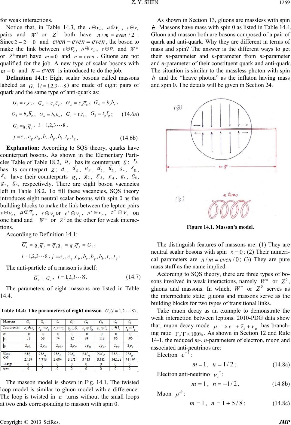

Z. Y. SHEN 1269
for weak interactions.
Notice that, in Table 14.3, the e
e

,



,




pairs and 
Wor 0
Z
both have 2// evenmn.
Since 022 and eveneveneven  , the boson to
make the link between e
e

,



,

  and 
W
or 0
Z
must have 0m and evenn . Gluons are not
qualified for the job. A new type of scalar bosons with
0m and evenn is introduced to do the job.
Definition 14.1: Eight scalar bosons called massons
labeled as i
G (83,2,1i) are made of eight pairs of
quark and the same type of anti-quark as:
rrccG  1, ggccG 
2, bbccG

3, rr bbG 
4,
gg bbG  5, bbbbG 
6, rrttG 7, ggttG 
8; (14.6a)
jjiqqG , 83,2,1 i,
grbgrbgr ttbbbcccj ,,,,,,,. (14.6b)
Explanation: According to SQS theory, quarks have
counterpart bosons. As shown in the Elementary Parti-
cles Table of Table 18.2, r
u has its counterpart
g
; b
t
has its counterpart
Z
; r
d, g
d, g u, b
d, b u, r
s, g
s,
b
s have their counterparts 1
g, 2
g, 3
g, 4
g, 5
g, 6
g,
7
g, 8
g, respectively. There are eight boson vacancies
left in Table 18.2. To fill these vacancies, SQS theory
introduces eight neutral scalar bosons with spin 0 as the
building blocks to make the link between the lepton pairs
e
e

,



,



or e e  
,

 
,

 
 on
one hand and 
W or 0
Z
on the other for weak interac-
tions.
According to Definition 14.1:
ijjjjjjiGqqqqqqG  ,
83,2,1i,grbgrbgr ttbbbcccj ,,,,,,,.
The anti-particle of a masson is itself:
ii GG, 83,2,1 

i. (14.7)
The parameters of eight massons are listed in Table
14.4.
Table 14.4: The parameters of eight masson )82,1(




iGi.
The masson model is shown in Fig. 14.1. The twisted
loop model is similar to gluon model with a difference:
The loop is twisted in n turns without the small loops
at two ends corresponding to masson with spin 0.
As shown in Section 13, gluons are massless with spin
h. Massons have mass with spin 0 as listed in Table 14.4.
Gluon and masson both are bosons composed of a pair of
quark and anti-quark. Why they are different in terms of
mass and spin? The answer is the different ways to get
their m-parameter and n-parameter from m-parameter
and n-parameter of their constituent quark and anti-quark.
The situation is similar to the massless photon with spin
h and the “heave photon” as the inflaton having mass
and spin 0. The details will be given in Section 24.
Figure 14.1. Masson’s model.
The distinguish features of massons are: (1) They are
neutral scalar bosons with spin 0s; (2) Their numeri-
cal parameters are 0// evenmn

; (3) They are pure
mass stuff as the name implied.
According to SQS theory, there are three types of bo-
sons involved in weak interactions, namely 
W or 0
Z
,
gluons and massons. In which,  W or 0
Z
serves as
the intermediate state; gluons and massons serve as the
building blocks for two types of transitional links.
Take muon decay as an example to demonstrate the
weak interaction between leptons. 2010-PDG data show
that, muon decay mode

 e e

has branch-
ing ratio %100/ i. As shown in Section 12 and Rule
14-1, the reduced m-, n-parameters of electron, muon and
associated anti-neutrinos are:
Electron  e:
1

m, 2/1

n; (14.8a)
Electron anti-neutrino 
e

:
1

m, 2/1

n. (14.8b)
Muon 

:
1

m, 8/51 

n; (14.8c)

Z. Y. SHEN 1270
Muon anti-neutrino 


:
1m, )8/51(

n. (14.8d)
In (14.8), the arrows  in particle symbols indicate
these particles with right-handedness.

W serves as the intermediate state with reduced m-,
n-parameters as:

W gauge boson:
2m, 14n. (14.9)
The “-” sign of n-parameter for 
W is due to the fact
that 
W is the anti-particle of  W.
According SQS theory,

  e e decay
mode includes two processes with two links: Process-1
with link-1:   W


; Process-2 with link-2:
e
eW    . In process-1,


to replace


is to
represent the leptons pair of

 
 required by Rule
14.1. In presentation,


serves as an input. In reality of
muon’s decay,


serves as an output. According to
Feynman diagram,


as input and


as output are
equivalent. Look it the other way, for process-1,
  W


takes the


as an input from a



& pair out of vacuum to avoid violation of lepton
number conservation and leaves the


as decay prod-
ucts. In this way, 
W boson status is justified and the
lepton family number conservation law in process-1 and
process-2 both are satisfied.
The two processes are illustrated in Table 14.5 to show
the makeup of two links.
Table 14.5A. process-1 for muon decay mode


e
e

 .
Table 14.5B. Process-2 for muon decay mode


e
e

 .
As shown in Table 14.5A and B, the weak interaction
in the muon decay mode


e
e
 has two links and
both links are made of three massons 1
G, 5
G and 6 G.
Take the free neutron decays to proton as an example
to demonstrate the weak interaction involved baryons
and leptons. According to 2010-PDG data, free neutron
decay mode e
epn    has branching ratio
%100/i. The mechanism of such decay is a down
quark in the free neutron transforms into an up quark
changing neutron to proton plus an electron and an elec-
tron anti-neutrino: e
eud   . The decay mode
also has two processes with two links and an intermedi-
ate state. As shown in Section 11, the m-, n-parameters of
three up anti-quarks and three down quarks are:

r
u: 1

m, 1


n; 
g
u: 7m, 3n;

b
u: 13

m, 5


n. (14.10)

r
d: 3

m, 1

n; 
g
d: 5m, 3n;

b
d: 11

m, 5

n. (14.11)
In (14.10), bgr uuu ,, to replace bgr uuu,, has the
same reason as


to replace


in the first example.
The two processes are illustrated in Table 14.6 to show
the makeup of two links.
Table 14.6A. Process-1 for down quark decay mode e
eud 

 .
Table 14.6B. Process-2 for down quark decay mode e
eud 

 .
In this example, the process-1 is quark and anti-quark
transforms to 
W mediated by gluons. The process-2 is

W transforms to leptons mediated by massons.
These two examples serve as the typical cases for the
regular weak interactions. The examples show that Rule
14.1 serves the purpose well. Other cases can be treated
by the same way.
For the rarely occurred weak interactions, the violation
of baryon number conservation and/or lepton number
conservation will be treated differently.
Definition 14.2: The weak interactions are classified
into two types.
Regular type: The weak interactions meet baryon
number conservation and lepton number conservation in-
cluding lepton family number conservation.
Rare type: The weak interactions violate baryon num-
ber conservation or lepton number conservation includ-
ing lepton family number conservation.
The weak interaction mechanism proposed by SQS
theory has following features.
1) It is based on mathematics. SQS theory provides a
mathematic framework for weak interactions.
2) In general, the rules introduced in this section meet
the requirement of baryon number conservation. A single

Z. Y. SHEN 1271
quark or anti-quark cannot participate in regular weak
interaction, because its oddoddmn //

. To partici-
pate in regular weak interaction, quark must pair with
anti-quark to have combined parameters of
evenevenmn // .
3) In general, the rules introduced in this section meet
the requirement for lepton number conservation includ-
ing lepton family number conservation. A single lepton
or anti-lepton cannot participate in the regular weak in-
teraction, because its oddfractionalmn// . To par-
ticipate, the lepton is paired with its companion an-
ti-neutrino to form a pair. The pair’s 2/0/

ppmn
along with 2/14/ 
WW mn of 
W or 0
Z
yield a
combined 0/)/()(/ evenmmnnmn WpWpcombcomb  ,
which naturally requires massons with 0//evenmn to
serve as building blocks of the link between them. In this
way, the lepton number and lepton family number are
conserved, and the introduction of massons is justified.
4) For SQS theory, the conservation laws for baryon
number and for lepton number including lepton family
number are required by mathematics represented by Rule
14.1.
5) The rules introduced in this section are also appli-
cable to some rare events. For instance, according to
2010-PDG data, the meson 0

has two rare decay
channels:  eeee with 5
10)16.034.3(/ i
and ee with 8 10)33.046.6(/  i. For these
two decay channels, there is no anti-neutrino involved,
but lepton numbers including lepton family number are
conserved. Because 0

is made of 2/)(
0dduu 

,
the explanation for its quark and anti-quark part is similar
to that of free neutron decay case. For the leptons part,
the n/m ratio of 
e is 2/)2/1(/

mn, which is the
same as e

. The explanation for the leptons part is the
same as two previous examples. But 
e is not e

, Rule
14.1 is violated and the decay mode belongs to rare type.
6) It also provides possible mechanisms for the rare
weak interaction events which violate lepton family
number conservation. For instance, according to 2010-
PDG data, 0

has three other very rare decay channels:
channel-A,  e

0 with 10
108.3/ i; chan-
nel-B,  e

0 with 9
104.3/  i; channel-C,
  ee

0 with 10
106.3/  i. Let’s take a
look at channel-A. the m-parameters and n-parameters
involved are:
For 

:
1
 
m, 8
13
8
5
1
 
n,
1
8/13






m
n; (14.12a)
For  e:
1

e
m, 2/1

e
n,
1
2/1

e
e
m
n; (14.12b)
For 
0
Z
:
2
0

Z
m, 14
0

Z
n;
2
14
0
0
Z
Z
m
n. (14.12c)
In this case, the problem is that, the n/m values of
(14.12) do not match as the way e
e 


 did in Table
14.5B. To solve the problem, let’s multiply numerator
and denominator of mn/ with 8 and 10 for 

and

e, respectively.
For 

:
8
13
8
8
'
'













m
n
m
n, (14.13a)
For 
e:
10
5
10
10
'
'



e
e
e
em
n
m
n, (14.13b)
For  e

:
2
18
108
513
''
'' 







e
e
mm
nn


. (14.13c)
The process-2 with link-2 can be carried out the same
way as previous examples.
For   eZ

0:
0
4
22
1814
)''(
)''(
0
0









eZ
eZ
mmm
nnn


. (14.14)
The link of (14.14) can be made of 62
3GG with
003
118383
0
4





. (14.15)
The same approach is applicable to channel-B and
channel-C. Is multiplication of same number to numera-
tor and denominator of mn/ legitimate? From math-
ematic viewpoint, the answer is: Yes, of cause. If the
reduction for the original mn/ is legitimate, so is the
multiplication. From physics viewpoint, the multiplica-
tion of an integer N to numerator and denominator of
mn / means that, the cyclic movements in loop-1 and
loop-2 both take N cycles instead of 1 cycle. For instance,
in the case of (14.13), the process occurred at the mo-
ment that,   takes 8 cycles and 
e takes 10 cycles.
The probability for such events occurred simultaneously
determines the


/
ivalue for that decay channel, which
explains the rarity of such decay channels.
7) The extremely rare “sphaleron” phenomenon [13]
converts three baryons into three leptons which violate
both baryon number conservation and lepton number
conservation. Three baryons contain nine quarks. The
combination has oddoddmn //

, which serves as the
mathematical origin for violating baryon number con-
servation. Three leptons combination has

Z. Y. SHEN 1272
oddfractionmn //,
which serves as the mathematical origin for violating
lepton number conservation. The regular rules introduced
in this section are not valid. But as long as multiplication
can apply to mn/, the “sphaleron” phenomenon can be
interpreted mathematically. In fact, almost any weak in-
teraction rare event can be interpreted mathematically.
The real difference is the probability of its occurrence.
These features indicate that, the weak interaction rules
have the capability and potential to explain weak interac-
tions in terms of mathematics. But there are some ques-
tions.
1) Is it possible that gluons and massons bypassing

W and 0
Z
directly link quark-antiquark pair to lepton
pairs e
e

,



 or



 ?
2) Massons are scalar bosons. Are they qualified to
serve as mediators for weak interactions?
3) Why gluons and massons are different? After all,
both are quark anti-quark pairs and located in the same
row in the Elementary Particles Table of Table 18.2.
4) 1 Y and 2 Y having mass around 2 /6.45 cGeV are
originated from g
t and b
t having mass around
2
/1.171cGeV. There is a reversed mass gap between
them. What’s to do with the mass gap?
Question-1 and Question-2 are correlated. If massons
must attach to 
W and 0
Z
, it answers both questions. In
fact, there are clues for massons attachment to 
W and
0
Z
. If the )2(SU group symmetry associated with
electroweak interaction is perfect, 
W and 0
Z
have no
mass. The )2(SU symmetry must be broken for 
W
and 0
Z
to gain mass. Massons may play a role to pro-
vide mass for breaking the symmetry.
Regarding Question-3, the spin and mass differences
of gluon and masson are originated from their models as
explained previously.
The answer of Question-4: The reversed mass gap of is
filled by massons some of them with negative sign. The
negative sign for massons is permitted as shown in Table
14.5 and Table 14.6b. It shows that massons are in some
way attached to 
W and 0
Z
.
Superficially, the introduction of eight massons seems
to make theory complicated. In fact, it is just the opposite.
The way SQS theory treated strong interaction and weak
interaction is to reveal their mathematic nature in the
simplest possible way. Gluons and massons both are
made of quark and anti-quark pairs. This approach
greatly simplified the theory. From SQS theory view-
point, quarks and anti-quarks serve as the basic elements.
Gluons and massons are composed with the basic ele-
ments in different ways to serve their specific purposes.
Moreover, the mathematic framework of weak and
strong interactions are self-consistent without artificial
additions. The whole approach shows simplicity and
elegance.
In Section 18, a new gauge boson will be introduced.
It also plays some role for the weak interactions involved
hadrons decay.
In this section, a framework of weak interactions is in-
troduced. It has the capability and potential to explain
weak interactions including rear events based on mathe-
matics. But it only provides a framework; some details
need to be finalized. For instance, the different ways 1
Y
and 2
Y are combined to make 
W and 0
Z
with dif-
ferent masses, which need more works to nail down the
details.
Section 15. Unified Interactions
Traditionally Grand Unification Theory (GUT) is to uni-
fy electromagnetic, weak, strong interactions, in which
gravity is not included. For SQS theory, GUT means
unification of all four interactions including gravity.
The unification of interactions takes consecutive stages.
Starts from electromagnetic interaction, weak interaction
joints in, then strong interaction joints in, finally all in-
teractions are unified with gravity. The GUT provided by
SQS theory is based on mathematics.
In

 xEDSx
 of (9.3), the second summation term not
included in the original DS-function of (6.1) represents
interactions mediated by bosons, which are originated
from Fourier transformation of the added

-function
terms in

 kEDS k of (9.1). For convenience,

 xEDSx

is divided into four summation terms labeled as A, B, C, D:

 
 

.,
,
2
1
,
2
1
;
2
1
2
1
)5.0(4)5.0(444
)5.0()(
5.045.0444
)5.0(
22
2 2
2
2
22
































j
xjij
j
xjij
j
xj
j
xj
j
xjij
j
xjij
j
xj
j
xj
x
eeDeeC
eBeA
DCBAeeee
eexEDS





(15.1)
Term-A and term-B represent fermions, while term-C
and term-D represent bosons for interactions.
According to their variables
j
and )5.0( j

versus
x
and )5.0(x

, term-C and term-D are related to
term-A and term-B, respectively. If the term-A variable
x
is in the )25.00(


x range with


)(x; then
the term-B variable )5.0( x

is in the

 5.0)5.0(25.0 x
range with




)5.0( x. For the torus model,


)(x
and




)5.0( x correspond to its inner half and outer
half, respectively. It implies that, term-B and term-D
corresponding to torus outer half are related to the
GWS-triangle representing electroweak interaction. It is

Z. Y. SHEN 1273
natural to assume term-D related to electroweak interac-
tion. With the same reason, term-A and term-C corre-
sponding to torus inner half are related to the
CKM-triangle representing hadrons decay. It is natural to
assume term-C related to electroweak and strong interac-
tions. Let’s take this argument as pre-assumption and
verify it by its results later.
In the )5(SU Grand Unified Theory [14,15], a sup-
pression factor SF is introduced:
4







GUT
proton
M
M
SF . (15.2)
2
/)23(938272013.0 cGeVM proton 
is the proton mass; and
215 /10~ cGeVMGUT
is the )5(SU GUT mass scale for the unification of three
interactions except gravitation. In a previous paper [16],
the author borrowed this concept and utilized (15.2) to
calculate the mass scale ew M for the unification of elec-
tromagnetic and weak interactions:
4ew
proton
ew SF
M
M. (15.3)
In which, ew
SF is the redefined suppression factor for
electroweak unification derived from the dominate term
of term-D in (15.1), in which
x
is replaced by b
x and

is replaced by )( b
x

:
937019456.20
)(
10
)()5.0(4)5.0)((4
104234326.1
2






e
eeeSF bbbb x
orj
xxjijx
ew

.(15.4)
The term with 10 orj  represents the dominate
term, which has the maximum magnitude value in
term-D. It dominates the suppression effect, because oth-
er terms with 1j have much less value comparing to
10 orj  term. In (15.4), the value of
5
108477191821861791.1  
b
x
is defined by (2.22), the value of
37019456.20)( 
b
x

is cited from Table 3.1, in which only 8 digits after the
decimal point are taken.
Substituting (15.4) into (15.3) yields the mass of a
scalar boson 1
U to unify electromagnetic and weak
interactions:
2
49
4/75469.152
104234326.1
938272013.0 cGeV
SF
M
M
ew
proton
ew 

 . (15.5)
2
/75469.152 cGeVM ew  is within LHC capability, it
can be verified experimentally.
Corresponding energy GeVcMEewU 75469.152
2
1
of the scalar boson 1
U serves as the energy scale to
unify electromagnetic and weak interactions.
The suppression factor ews
SF for electroweak-strong
unification is derived from the term-C of (15.1). It is
evaluated at
10
10882111819946879.5  
a
x of (2.21)
and cited from Table 3.173631245.36)( 
a
x

with
8 digits after decimal point:
6473631245.364 )(4
1
)(4)(4 1052226012.1
2


  eeeeSF aaaa x
j
xxjijx
ews

.
(15.6)
In (15.6), the 1j term is taken as the dominate
term instead of the 0

j term, because 0

j term
represents the summation of all probabilities equal to 1
required by unitarity.
Using the value of ews SF giving by (15.6), the mass
ews
M of a scalar boson 2
U to unify electroweak and
strong interactions is determined as:
215
16)(
4
/1044708.8
1011076508.1
938272013.0 cGeV
e
M
SF
M
Ma
x
proton
ews
proton
ews 



.
(15.7)
In standard model, the electroweak-strong unification
is called the grand unification. In SQS theory, the grand
unification is reserved for the one including gravity.
Before dealing with the grand unification, let’s look at
the principles suggested by SQS theory.
1) There are two types of forces (force is synonymous
to interaction). The long range force including electro-
magnetic force and gravitational force, both have unlim-
ited effective range. The short range force including
weak force and strong force has limited effective ranges.
The first principle for grand unification is: All forces
must be unified to a single force of the long range type.
The reason is simple, long range includes short range,
while short range does not include long range. According
to the first principle, the weak force and strong force are
not qualified as the final unified force.
2) Second principle: The force with selectivity is not
qualified as the final grand unification force. Electro-
magnetic force is only for charged particles. It is not
qualified as the final unified force. Otherwise, the forces
between electrically neutral particles are left out after the
grand unification.
3) According to the first and second principles, the
only force qualified as the final unified force is the grav-
ity.
The next question is: In the grand unification, which
force is one finally unified with gravity? The answer
comes from the Random Walk Theorem. In Section 4,
the ratio of electrostatic force to gravity for a pair of
electrons is
2
2
/4e
G
E
GE N
f
f
R


 . (4.19)

Z. Y. SHEN 1274
In which, electron converting factor e
N is interpreted
as the ratio of long path to short path defined according
to the Random Walk Theorem. It is natural to start with
GE
R/ to explore grand unification. According to SQS
theory, grand unification happens at:
1/
/GEGEffR. (15.8)
Substituting (15.8) into (4.19) yields:


2

e
N. (15.9)
In (15.9), the fine structure constant

as a running
constant varies with energy. The closest value available
at such high energy level from 2010-PDG (p.126) is:

015.0916.127/1)( 
Z
M

. (15.10)
)( Z M  is the value of

at 22 Z
MQ  around GeV91 .
Substituting (15.10) as

into (15.9) yields the con-
verting factor at grand unification scale:
06279805.71
)(
2
Z
GUT
Planck
GUT M
M
M
N


. (15.11)
Corresponding length is the grand unification length
scale:
mLNLPGUTGUT 3335 10148552.11061625.106279805.71  .
(15.12)
The mass of the scalar boson 3
U for grand unifica-
tion is:
2189 /1007948213.1109243515.1
2
)(
2
)(
cGeVKg
G
hcM
M
M
N
M
MZ
Planck
Z
GUT
Planck
GUT







. (15.13)
For comparison, the suppression factor GUT
SF and
)( GUT x

for grand unification are reversely calculated
from GUT
M as:
73
4
18
4
1070759593.5
1007948213.1
938272013.0 
















GUT
p
GUT M
M
SF ,
(15.14a)
58672847.41
4
)ln(
)( GUT
GUT SF
x 
. (15.14b)
Table 15.1 listed the calculated parameters for three
types of unifications proposed by SQS theory.
Table 15.1. The parameters for three types of unifications.
*Note: 58672847.41)( 
GUT
x

and 73
107076.5  
GUT
SF are reversely
calculated from GUT M .
It is interesting to find out that, the mass ratio of
GUT
M to ews Mis very close to 1
)( 
Z
M 
:
1
)(79353.127   Z
ews
GUT M
M
M

. (15.15)
The number 79353.127 is so close to the medium
value of 916.127)( 1

Z
M 
cited from 2010-PDG
(P.126) data with a relative deviation of 4
10574.9 .
Another way to check is to combine (15.13) and (5.15):
83433738.127
2
)(
3/2
1








ews
Planck
ZM
M
M


. (15.16)
The relative deviation is reduced to4
10384.6  . With
such high accuracy, it is very unlikely that (15.15) and
(15.16) are by coincidence. In other words, these correla-
tions are real and mean something worthwhile to dig in.
From theoretical perspective, (15.15) is an important
finding, which has the following significances.
1) The parameters of grand unification and elec-
troweak-strong unification are correlated with the fine
structure constant)( M

. )(M

as a running constant, its
reversed value varies from 035999084.137)( 1

e
M 
to 916.127)( 1

Z
M 
, a decrease of %655.6 for 5
10~
increase of energy scale. In the next 16
10 increase of
energy scale to GeV
18
10 , the value of 1
)( M 
is only
decreased 4
10384.6  . It shows a typical asymptotic
behavior toward saturation: )()( GUTZ MMM


 . In
other words, the majority of 4
10384.6   relative de-
viation is not necessarily caused by error.
2) Combining (15.15) and (15.16) and replacing
)( Z M

with )( GUT
M

yields the correlation of three
masses:
Planck
GUT
GrandGUTews M
M
MMM



2
)(
)(
2/3
 . (15.17)
Due to the asymptotic nature of fine structure constant,
the replacement of )(Z
M 
with )( GUT
M

in (15.17)
only has a minor effect.
3) More importantly, the finding proves an important
evidence for the consistency of two very different meth-
ods used to deal with unifications for SQS theory. ews
M
is calculated according to the suppression factor from
(15.6) and formula (15.7) as a borrowed formula, )( a
x

is originated from the S-equation. On the other hand,
GUT
Mis determined by the equality of static electrical
force and gravity along with the converting factor GUT
N
originated from Random Walk Theorem. These two very
different methods are consistent with a discrepancy less
than 4
10384.6  . It gives the legitimacy for both meth-
ods. After all, the borrowed formulas (15.3), (15.5) and
(15.7) are legitimate; and the ways to determine suppres-
sion factors by )( a
x

and )( b
x

are legitimate as well.
It gives more credit to the theoretical results listed in
Table 15.1.
4) It proves a way to convert proton mass proton
M and

Z. Y. SHEN 1275
converting factor proton
N to the Planck mass Planck
M.
Substituting ews
M of (15.7) into (15.17) yields:
Planck
x
GUTproton MeMM a)(
2/3
)(
2
1




, (15.18a)
)( 2/3
)(
2
a
x
GUTproton
Planck
proton eMM
M
N




 . (15.18b)
Proton is not an elementary particle. It composed of
three quarks and many gluons. For such a complex sys-
tem, its mass and converting factor can be derived from
three mathematic constants,

, e, a
x and a running
constant )( GUT
M

by (15.18). It is a surprise. This
correlation is important in two senses. First, SQS theory
is based on three physics constants, h, c, G and in
principle no other physics inputs. The proton
M in (15.3),
(15.5), (15.7) is exceptional. With the help of (15.18a),
proton
M is replaced by Planck
M, proton mass is no longer a
physics input for SQS theory. Second, most formulas and
equations in this paper can be traced directly or indirectly
back to the first principle of SQS theory. (15.3), (15.5),
(15.7) are exceptions, which are borrowed from other
theory. With the help of (15.18), the problem is solved.
For instance, ews
M and ew M are expressed as:
G
hc
MM
M
MMMGUTPlanck
GUT
GUTGUTews





2
)(
2
)(
)( 2/3
2/3
 .
(15.19)

G
hc
e
M
M
e
M
M
e
M
Mbababaxx GUT
Planck
xxGUT
GUT
xx GUT
ew




2)(
2
)()(
4/)()(
2/3
4/)()(
2/3
4/)()( .
(15.20)
Only mathematic constants and basic physics con-
stants appear in (15.19), (15.20).
The value of converting factor GUT
N given by (15.11)
is twenty one orders of magnitudes less than electron
converting factor:
23
10501197.1/  Pee LN 
. (6.16)
The tremendous reduction of converting factor is the
nature of random walk. As shown in Section 4, when the
distance l of two electrons is equal or greater than its
Compton wavelength eC

, its converting factor is fixed
at 23
10501197.1/ Pee LN 
, which is represented by
a flat straight line on the )(lNe versus ldiagram shown
in Fig. 4.1. This is the macroscopic scenario. When the
distance of two electrons is reduce to eC
l

, the con-
verting factor )(lNe starts to vary. According to Ran-
dom Walk Theorem, the number of steps along the ran-
dom walk path rw
n is
2
strw nn . (15.21)
st
n is the number of steps along the straight line distance
between two electrons. The ratio of random path length
and straight line distance is:
ststrwstrw nnnR 

/
/. (15.22)
strw
R/ is linearly decreases with decreasing st n. In this
region, )(lNe has a linear relation with l, which is
represented by a straight line with 
45 angle to the
l-axis in )(lNe versus l diagram shown in Fig.4.1.
The line stops at the grand unification length scale given
by (15.12): mLNL PGUTGUT 33
1014855.1   . This
process has its deeper meanings, which will be discussed
in Section 16.
As a summary of this section, let’s look at the process
of unifications.
1) The electrical force and magnetic force are unified
by Maxwell equations with no specific length scale.
2) At the length scale mLew 18 1011656.8   , weak
force joints with electromagnetic force to unify as elec-
troweak force.
3) At length scale mLews 31
1046778.1   , strong force
joints with electroweak force to unify as elec-
troweak-strong force.
4) Finally, at length scale mLGUT 33
1014855.1   ,
electroweak-strong force is unified with gravity, and all
four forces become one.
In the consecutive stages of the unifications process,
the electromagnetic force, acting as the carrier, picks up
other forces at different length scales and carries them to
the final stage. At the final stage, all forces are united to
gravity. This process follows the principles described at
the beginning of this section.
The electromagnetic force acting as the carrier has a
deep reason. It is the force has direct connection with
gravity via the random walk process. This is another
example to show the importance of the Random Walk
Theorem and its origin, the SQS theory Fundamental
Postulation of Gaussian Probability.
In some other source [17], fine structure constant at
Z
M has a value 020.0957.128)(
1 Z
M 
different
from PDG-2010 015.0916.127)( 1

Z
M 
. The dis-
crepancy indicates a different asymptotic path from
1
)( 
Z
M 
towards 1 )( 
GUT
M  . It does not change the
conclusion of the intrinsic link betweenews
M and GUT M.
In Section 23, the unification length scales ews
L and
GUT
L serving as milestones play important roles in cos-
mic history.
In Section 24, a universal formula for the fine structure
constant )(M

will be given.
Section 16. Logistic Equation and Grand
Numbers
In this section, an equation is discovered by 16-digit nu-
merical calculation. It reveals the connections among
logistic recurrence process, converting factor, Gaussian
probability, random walk, S-equation and grand number

Z. Y. SHEN 1276
phenomena. It also provides important clues related to
vacuum structure, cosmic history and finite sporadic Lei
group.
In Section 15, the converting factor of the scalar boson
3
U representing the grand unification is:
06279805.71)(2 1 ZGUT MN 
. (15.11)
An equation is discovered by using 16-digit numerical
calculation, which provides connection of the electron
converting e
N to other constants:
0106062632564145.4)(22141
)(2
1 
e rx
eMeN


.
(16.1)
Equation (16.1) is not derived from the first principle.
It is necessary to provide all information in details. On
(16.1) right side, the number 14
106062632564145.4  
is restricted by the resolution of 16-digit numerical cal-
culation. It actually equals to zero. The values of two
terms on left side of (16.1) are:
3825524601809.7322
1)( 
rx
eeN

, (16.2a)
3825524601809.73)(21
e
M 
. (16.2b)
It proves the right side of (16.1) actually equal to zero,
which serves as one of evidences that equation (16.1) is
not by coincidence.
In (16.1), the following constants are cited from the
medium value of 2010-PDG data, or derived from the
S-equation.
Electron converting factor:
ePlancke MMN /, (16.3a)
Planck mass:
cL
h
M
P
Plank, (16.3b)
Planck length:
mLP35 1061625.1   , (16.3c)
Electron mass from 2010-PGD data:
kgMe31 1010938215.9  , (16.3d)
Planck constant from 2010-PDG data:
Jsh34 1062606896.6 , (16.3e)
Speed of light in vacuum from 2010-PDG data:
smc/1099792458.28  , (16.3f)
From 2010-PDG data (p.126):
035999084.137)(
1 e
M 
, (16.3g)
From S-equation solution for electron:
200378771029244.3)125.0()(1  x. (16.3h)
In Appendix 5, a brief introduction of logistic equation
is presented.
r
is a parameter of the logistic equation:
)1(
1iii xrxx


, 3,2,1,0i. (A5.3)
Logistic equation represents a recurrence process with
close connection to chaos theory. i
x as a function of
r
demonstrates different behaviors in different regions of r
shown in Table 16.1.
Table 16.1. The typical behaviors of i x in different ranges
of
r
values.
In (16.1), the logistic parameter is:
3244445700363330.3




rrrc. (16.4)
5699457.3

c
r, (16.5a)
5
1006330324.9 r. (16.5b)
c
r is the threshold of parameter
r
. When c
rr, the
logistic recurrence process becomes chaotic.
In the equation (16.1), as shown by (16.5), the differ-
ence between parameter
r
and c
r is
5
1006330327.9 r.
The relative deviation is:
5
10539.2/   c rr . (16.6)
The value of
r
just a litter bit more than the thresh-
old of 5699457.3

c
r. At that point and beyond, the
logistic recurrent process becomes chaotic.
It is important to point out that, 5
10539.2/   c rr
does not all contribute to the error of (6.1). In fact,
r

could be interpreted as the logistic recurrent process go-
ing into chaotic region a coup of more steps. The error of
(16.1) is less than 5
10536.2/   c rr. With such high
accuracy, equation (16.1) cannot be by coincidence. We
should take it seriously and dig in deeply.
The second term on the left side of (16.1) is:
3825524601809.73)(2 1
e
M 
. (16.2b)
Obviously, (16.2b) is the electron version of (15.11)
with the )(Z
M 
replaced by )(e
M

at electron mass
scale as it should be.
Let’s look at the logistic equation (16.1) as a progres-
sive process with
r
as a variable. To show )(rNe as a
function of
r
. Rewrite (16.1) as:
0)(2)(2 1
)( 2
1
MerN rr
e


. (16.7)
In (16.7), )(
1M 

is a running constant. The prob-
lem is that )(
1M 

value varies with mass scale M. The
experimental data of )(
1M 

are available only at a

Z. Y. SHEN 1277
couple of discrete points. 2010-PDG (p.126) data pro-
vides:
035999084.137)(
1 e
M 
. (16.3g)
In Section 15, the value of )(
1Z
M


is cited from
2010-PDG (p.126) data as:
015.0916.127)(
1 Z
M 
. (15.10)
Fortunately, as shown in Section 15, above Z M mass
scale the value of )(
1Z
MM 


asymptotically ap-
proaches saturation. Table 16.2 lists the related parame-
ters as a function of
r
. In which, )(
1e
M


is used at
2
cM e energy scale and )(
1Z
M


medium value is used
for at and beyond 2
cM Z energy scale and its variation is
ignored.
Table 16.2. Parameters of electron logistic process.
In Table 16.2, the logistic recurrent process belongs to
the variable parameter type, in which parameter
r
var-
ies. It starts at 29898133.0r and stops at
57003633.3r.
In the process, besides the three milestones, 1

r
,
2
r
, 3r, the other milestones correspond to elec-
tro-weak, electroweak-strong and grand unifications are
also listed. The term with
11
10874529.3)(  ee NrN
corresponds to electron intermediate state, the e-boson
state, related to cosmic inflation will be explained in Sec-
tion 23.
Table 16.2 clearly demonstrates the dynamic nature of
electron converting factor )(rN e. It provides a convinc-
ing interpretation of )(rN e as a running constant. In
essence, the variation of )(rN e is a random process
originated from two correlated sources. One is the ran-
dom walk process described in Section 4 and the other is
the logistic recurrent process. In fact, i
x and )1( i x

of
(A5.3) can be interpreted as binary probabilities. In some
way, i
x and )1( i
x are related to the probabilities in
the random walk. The details of the correlation are up to
further exploration.
With the help of logistic process, the peculiar behavior
of )(lNe in Section 4 is understood now. Why
)( ee lN

 is a running constant? Because its logistic
process belongs to the varying
r
parameter type. Why
)( eCe lN

 does not show asymptotic behavior? Be-
cause the logistic process abruptly stops at rrrc



and becomes chaotic.
This is the hidden scenario revealed in this section.
Logistic recurrent process not only provides reasonable
explanation for the peculiar behaviors of the converting
factor )(lNe, but also links it to other constants such as
c
r
and )(M

.
In Table 16.2, at the starting point of logistic process,
06279805.71)29898133.0(


rNe. (16.8)
It is the same as:
06279805.71
)(
2
Z
GUT
Planck
GUT M
M
M
N


. (15.11)
06279805.71

GUT
N is the converting factor for sca-
lar boson 3
U representing grand unification, while
06279805.71)29898133.0(


rNeis electron’s convert-
ing factor at GUT scale. Why are these two numbers
equal? The apparent reason is that they use the same
)916.127/(1)( 
Z
M 
. The deeper reason is that, at the
GeVcM GUT 182 10~ energy scale, electron mass is in the
same order of 3
U mass, which far exceeds Max M. Ac-
cording to Rule 6.1, such heaver fermions must appear in
pair; and a pair of fermions is a boson. It demonstrates
the consistency of (15.11) from grand unification and
(16.8) from logistic process of electron.
Equation (16.1) is for electron. The corresponding taon
version is:
01044441263880373.3)(22 131
)( 2
11  






MeNrx .
(16.9)
The data in (16.9) are from the following sources:
From 2010-PDG data:
19
1031732.4/

MMNPlanck , (16.10a)
From 2010-PDG data: 015.0444.133)( 1


 M, take
444.133)( 1


 m. (16.10b)
From S-equation:
268531416714823.3)526282499640520.0()( 1 

x.
(16.10c)
The numerical solution of (16.9) for
 1
ris:

rrr c



1, (16.11a)
2
101734618773401.5  

r, (16.11b)
2
11053.1/ 


rr . (16.11c)
Comparing to the electron case, the value of

rrrc



1 is increased. It means that for taon the
logistic recurrent process goes further into the chaotic
region before it stops.
Consider electron macroscopic converting factor e
N

Z. Y. SHEN 1278
and its square root e
N in orders of magnitude:
11
1087.3~
e
N, (16.12a)
23
105.1~
e
N. (16.12b)
e
Nand e N are grand numbers representing typical
hierarchy phenomena, which deal with the ratio of two
quantities having many orders of magnitude difference.
There are other phenomena related to great numbers. For
example, the total number of stars in a galaxy is close to
11
10 ; the total number of galaxies in the visible universe
is close to 11
10 . More examples will be given in later
sections.
Definition 16.1: The Rank-G grand number is defined
as:
G
G
N11 10~ . (16.13)
A system consists of G
G
N11 10~ elements is defined
as a rank-G grand system. A grand system subjects to the
following conditions:
1) The elements in the system belong to the some type;
2) The interaction of elements in the system is weak;
3) The elements in the system behavior stochastically;
4) The interaction of elements is nonlinear in nature,
and it provides a growth mechanism with negative feed-
back. In fact, in (A5.3), i x represents growth and
)1( i x represents negative feedback to suppress growth.
Explanation: The grand number defined by (16.13) is
based on decimal for convenience, which is not natural.
The natural way to define it is:
g
G
N37 2~ , (16.14a)
1137 10374.17213743895342 . (16.14b)
The relations between
g
and G are:
GGg 259739876002444.0
)2ln(37
)10ln(11 


, (16.15a)
ggG 606660125554399.1
)10ln(11
)2ln(37


. (16.15b)
For practical reasons, definition (16.13) is introduced
and used throughout in the paper. Definition (16.14)
serves as its natural origin. It is interesting to notice that,
2 and 37 both are prime numbers.
According to Definition 16.1, galaxy is a 1

G grand
system with 11
10~ stars and the visible universe is a
2G grand system with 22 10~ stars.
The common feature of grand systems containing
grand number of elements is related to the logistic recur-
rence process. When the random process in the system
reaches the critical point 5699457.3

c
r, the system
becomes chaotic and stops growing. It can only grow
further by organizing a next higher level, such as the
visible universe on top of galaxies.
Since 23
105.1~ 
e
N is close to a 2G grand
number, a natural question is: What is the electron’s
1

G grand system with 11
1087.3~
e
N? This is an
important question, which will be discussed in Section
23.
Notice that, 7106279805.71

GUT
N deviates from
a prime number 71 with a relative deviation of
4
10837.8  . It is not by coincidence. In fact, it provides
a clue with important physics and mathematics signifi-
cances, which will be discussed in later sections.
The equation of (16.1) correlated ePlancke MMN / to
other mathematic constants. It has important significance,
which will be discussed in Section 21.
The only thing left unexplained is the numerical factor
2 in Equation (16.1) and (16.9). It turns out that the
factor 2 provides an important clue for the structure
of space and much more. The details will be discussed in
Section 22.
In summary, Equation (16.1) is an important discovery.
It reveals many important correlations including logistic
recurrence process, converting factor, Gaussian probabil-
ity, random walk, S-equation and grand number phe-
nomena. Some of them are worthwhile to explore further.
Section 17. Neutrinos
Neutrinos are puzzling particles with peculiar behaviors.
Despite extensive efforts in recent years tried to find out
neutrinos’ properties, some of them are still not clearly
known. In this section, only a framework is presented, in
which many issues remain open.
Let’s start with known facts.
Fact-1: Neutrinos have tiny mass evidenced by oscil-
lations among three different types.
Fact-2: Neutrinos only have left-handedness and an-
ti-neutrinos only have right-handedness.
Fact-3: Neutrinos have no electrical charge or tiny
remnant electrical charge.
The main focus of this section begins with
anti-neutrinos, because anti-neutrinos are the ones com-
panioned with their changed leptons and play a pivotal
role in most weak interactions.
Rule 17.1: According to the Leptons Pairing Rule in
Section 14, each charged lepton is paired with its com-
panion anti-neutrino: e
e

&,



&,



& with com-
bined numerical parameters evenm, 0

n; each
charged anti-lepton is paired with its companion neutrino:
e
e  &
,

 &
,

 &
 with combined numerical
parameters evenm


, 0n. The n-parameters mat-
ching rules are:
0


l
nnl

, or l nn l

,


,,el

,





,,
el ; (17.1a)
0


l
nnl

, or l
nnl

,

Z. Y. SHEN 1279

  ,,el,





,,
el . (17.1b)
Take electron anti-neutrino e

as an example. As
listed in Table 12.3, electron’s after reduction n-para-
meter is 2/1
e
n. According to (17.1a), the n-parameter
of e

is 2/1
e
n

, to make the match:
0)2/1(2/1 ee nn

. (17.2)
The e

as an anti-fermion, according to Definition
11.2, its m-parameter must have opposite sign of its
n-parameter:
0

eenm 
. (17.3)
Because of 02/1 
e
n

, e

must have 0
e
m

corresponding to e

right-handedness. The argument is
also applicable to the other two types of anti-neutrinos,


and


. It shows that, anti-neutrinos unique hand-
edness is hidden in Rule 17.1 and originated from ma-
thematics.
In reference [1] by the author, neutrinos were treated
based on their companion leptons and the
W
boson.
The mass values of three types of anti-neutrinos were
given as:

25
2
2
/102922.41
2ceV M
M
MM
W
e
ee 







 


, (17.4a)

23
2
/108749.81
2ceV M
MM
MM
W
e












,(17.4b)

21
2
/104925.11
2ceV M
MM
MM
W
e












.(17.4c)
In (17.4), the mass values, e M,

M,

M, W M and
the value of fine structure constant
035999084.137/1

are cited from 2010-PDG. e
M

,

M,

M are the
mass values of three flavored anti-neutrinos e

,


,


,
respectively, which are in principle different from the
eigenstate neutrinos 1
~

, 2
~

, 3
~

. The difference will be
discussed later in this section.
According to (17.4), the mass ratios of three
anti-neutrinos to their companion charged leptons are:

11
2
/103996.81
2









W
e
e
e
ee M
M
M
M
R 



, (17.5a)

11
2
/103996.81
2









W
e
M
M
M
M
R





, (17.5b)

11
2
/103996.81
2









W
e
M
M
M
M
R 




. (17.5c)
The three ratios are identical, which indicate that three
anti-neutrinos are closely related to their companion
charged leptons as well as among themselves.
To determine anti-neutrinos models and parameters,
two issues must be dealt with. One is mass and the other
is electrical charge, which are very different from their
companion charged leptons.
Let’s start from electron torus model and look for the
ways to transfer it into the model of its companion an-
ti-neutrino e

. According to SQS theory, the mass e M

of e

is related to its model and numerical parameters
in two ways.
1) According to (6.18) in Section 6, the distance be-
tween 1 x and 2 x on x-axis for e

is related to its
mass e
M

and electron mass e
M as:
eeee RMMxx /12 /1/4 
 . (17.6)
According to (17.5a) and (17.6):
9
/12109763.2)4/(1  ee
Rxx

. (17.7)
It indicates that, 1 x and 2 x are separated by a vast
distance alone x-axis. The values of )(1
x 
and )( 2
x 
are determined by 1 x and 2 x according to S-equation.
2) The numerical parameters m, n, p and the mass os-
cillation term in AT-, PS-equations are related to the
mass ratio.The mass ratio is defined as:
11
/103996.8 

e
e
ee M
M
n
p
R


, (17.8a)
The mass oscillation term is:





)/2(sin')/2(sin' /22 mnRampa ee

. (17.8b)
According to (17.8) and 1
e
m

, 2/1


ee nn

,
the way to reduce mass e
M

from e
M is to reduce the
value of the p-parameter:
1111
2
1
/101998.4103996.8   eeee Rnp 
. (17.9)
The numerical parameters of


and


can be de-
termine by the same way. The results are summarized as:
Electron anti-neutrino e

:
1

e
m

, 2/1


e
n

, 11
101998.4 
e
p

; (17.10a)
Muon anti-neutrino


:
1


m, )8/51(




n,10 103649.1  

p; (17.10b)
Taon anti-neutrino


:
1


m, )7/62(




n, 10
103999.2 

p.(17.10c)
For the electrical charge difference, the key is to let the
electrical charge to vanish for e

and keep all related
rules valid. As discussed in previous sections, particle’s
electrical charge q is related to Weinberg angle W

as
WW
q


cossin

. Let Weinberg angle 0
W

or
0

W

, the electrical charge follows 0q or 0

q.
Based on these considerations, SQS theory provides
two options for neutrinos model. The process starts from
torus model and followed by trefoil model for easy to
understand.
Option-1: For Dirac type neutrinos
In the electron’s torus model, move point
A
and
point '
A
to coincide with point G. As results, the torus

Z. Y. SHEN 1280
model and trajectory for e

are shown in Figure 17.1.
When point
A
and '
A
coincide with point G,
0
2

,  180
2

, 0
2

, 0
2

, and 0
2




W,
0q. In the outer half of torus cross section, according
to (8.8a),
A
and '
A
coincided with point Gmake
0
2Z, 0 2

and
1
2
)cos()sin(
2
2
2
2
2


Z
dttbta


, (17.11a)


)( 2 x. (17.11b)
In the region

5.0,0 of x-axis, the S-equation of (2.11)
has only one solution at
73026452499871562.0 c xx ,


)(c x. (17.12)
According to )(xS function’s periodicity of (2.12)
and symmetry of (2.13), (17.12) is extended to the entire
x-axis as:


 )( Nx c, 

3,2,1,0N; (17.13a)


 )1(Nxc, 

3,2,1,0N. (17.13b)
Figure 17.1. Torus model and trajectory for e

according
to Option-1.
According to (17.7) and (17.13), there are two ways to
determine 1
x and 2 x for e

.
Way-1:
c
xx

1,Nxx c


2;



 )()( 1c xx,






)()(2Nxx c; (17.14a)
Way-2:
c
xx

1, Nxx c


1
2;




)()(1c xx ,
  )1()( 2Nxx c. (17.14b)
In both ways,



)( 1 x and


)( 2 x, which are
required by probability matching.


)(1 x means
that, as point
A
and point '
A
coincided with point G,
point
B
and 'B also coincide with point E as shown in
Fig.17.1. The trajectory shown in Fig.17.1 is for e

. The
trajectory for e

has the same projections as the trajec-
tory for e

with opposite direction along the switched
solid line and dashed line on the x-y plane. The differ-
ences of two ways are:
For Way-1:
 NMMRxx eeee
e)4/(4/
/12 

integer, (17.15a)
For Way-2:
 ceeee
exNMMRxx 21)4/(
/12 

non-integer.
(17.15b)
Unfortunately, the accuracy of available data is not
sufficient to choose which way to go. In the meantime,
let’s take Way-1.
In the above discussion, e

serves as an example. The
same principles are applicable to


and


based on
the models of nuon and taon. Neutrinos e

,


,


share the some models as anti-neutrinos e

,


,


respectively with different trajectories’ directions.
Theorem 17.1: The Dirac type neutrino only with left
handedness and the anti-neutrino only with right hand-
edness must have zero electrical charge: 0



qq .
Proof: Let’s starts from the opposite. If 0


q and
0


q, then points
A
and points '
A
are not exactly
coincided with point G; point
B
and point 'B are not
exactly coincided with point E. In such case, there are
four possible trajectories, in which two trajectories for

with right and left handedness and two trajectories
for

with right and left handedness. This scenario vio-
lates Fact-2, which must be not true. Then the opposite
0



qq must be true. QED
The above discussions are based on torus model. The
real model for e

,


,


and e

,


,


are tre-
foil model with three branches. The way for three torus
models combined into a trefoil type model is the same
described in Section 12 for charged leptons. Figure 17.2
shows the trefoil type model and trajectory for e

.
The calculated parameters based on Option-1 trefoil
type model are listed in Table 17.1, 17.2, 17.3 for e

,


,


, respectively. The data are based on 0

q. The
after f-modification parameters are marked with ‘ .

Z. Y. SHEN 1281
Figure 17.2. Trefoil type model and trajectory for e

ac-
cording to Option-1.
The torus model and the trefoil type model provided
by Option-1 are only valid for Dirac type neutrinos and
anti-neutrinos with two components. There is a reason to
introduce Option-2 to provide a Majorana type model
with only one component, because eigenstate anti- neu-
trinos belong to Majorana type as shown later in this sec-
tion.
Table 17.1. Parameters for electron anti-neutrino based on
option-1.
Table 17.2. Parameters for muon anti-neutrino based on
option-1.
Table 17.3. Parameters for taon anti-neutrino based on op-
tion-1.
Option-2: For Majorana type neutrinos
Start from Option-1 torus model for e

with 0


q.
Let loop-2 center 2
O on right and center 2
'O on left
move toward loop-1 center 1
O and coincides with 1 O.
The torus surface becomes spherical surface for
1/22

ab or elliptical surface for 1/ 22 ab. In the new
model, loop-2 is integrated into loop-1. It fits the one
component Majorana type naturally. Spherical and ellip-
tical surfaces belong to genus-0 topological manifold.
The trajectory on torus surface is degenerated into a cir-
cle on the spherical surface or elliptical surface with
points G on its right and points E on its left as shown in
Figure 17.3.
The trajectory on trefoil type model is degenerated on
sphere surface or elliptical surface as shown in Figure
17.4. The model is degenerated from genus-3 to genus-0

Z. Y. SHEN 1282
without branches but the degenerated trajectory still re-
tains its 3-branch trefoil type with loop-2 integrated into
loop-1.
Figure 17.3. Torus model and trajectory degenerated to
sphere for 1
~

according to Option-2.
Figure 17.4. Trefoil type model and trajectory degenerated
to sphere for 1
~

according to Option-2.
In the process of weak interaction such as
e
epn  , an anti-neutrino is created with a defini-
tive flavor. The new born anti-neutrino flies with speed
very close to the speed of light in vacuum. During it fly-
ing journey, the anti-neutrino is oscillating among dif-
ferent flavors. In other words, the flying anti-neutrino
lost its flavor identity and becomes an oscillating system
of eigenstate anti-neutrinos. When it is caught by a de-
tector, the eigenstate anti-neutrino gets its flavor identity
according to probability. The oscillating behaviors were
found by experiments as the Fact-1, which serve as the
evidence for anti-neutrinos having tiny mass.
It is important to point out that, during their free flying
journey, the oscillation is among the members of eigen-
state version, and the members of flavored version only
show up at their birth or been detected. As soon as they
start to fly, the flavored version converts to the eigenstate
version.
Fine structure constant

is a running constant de-
pending on energy scales. In (17.4) and (17.5), the

value is based on the 2010-PDG (p.126) data:
035999084.137/1)(

e
M

. (17.16)
Take (17.4c) for


as an example, there are three
different energy scales involved. If

is treated as a
running constant, (17.4c) probably should be rewritten as:

21 /105318.1)(1
2
)(
2
)(ceV
m
MM
M
MM
M
W
e
Z
e


















(17.17)
In (17.17), 2010-PDG (p.126) data medium values are
used:
444.133/1)(



M, (17.18a)
916.127/1)(

Z
M

. (17.18b)
The difference between (17.4c) and (17.17) is
2
106.2  . The mass data listed in Table 17.1, 17.2 and
17.3 did not take

as a running constant into account,
which may have up to 2
10~errors.
According to 2010-PDG data, three charged leptons
have a mass relation:
50649.3


M
MMe. (17.19)
According to (17.4) and (17.19), if ignore the effect of

as a running constant, three anti-neutrinos have a
similar mass relation:
50649.3


M
MM e. (17.20)
(17.20) indicates that, three types of neutrinos are closely
correlated.
The neutrino models and parameters proposed by SQS
theory can be verified by checking on eigenstate neutri-
nos mass values. 2010-PDG provides the experimental
data for the differences of eigenstates mass squares:
2252
21 )/(10)
21.0
19.0
59.7(ceVM 



 , (17.21a)
2232
32 )/(10)13.043.2(ceVM 
 . (17.21b)
Which are based on 2010PDG assumption:
2
31
2
32 ~MM  . (17.21c)
According to (17.4), the SQS theoretical values are:
22522 )/)(10876.7(ceVMM e


, (17.22a)
22222 )/)(1022.2(ceVMM 


, (17.22b)
22222 )/)(10227.2( ceVMM e


. (17.22c)
The 22 e
MM

 theoretical value of (17.22a) is close

Z. Y. SHEN 1283
to the experimental 2
21
M value of (17.21a). The other
two are off by a factor of ~9 for mass square; for mass
without square, they are off by a factor of ~3. The as-
sumption 2
32
2
31 ~MM  of (17.21c) also fits (17.22b)
and (17.22c) well. But they are not fair comparisons. In
principle, e
M

,

M,

M as flavored anti-neutrinos
mass are different from eigenstates mass 1 M, 2 M, 3
M.
Nevertheless, the 2010-PDG data provided some tenta-
tive information. For instance, one possible interpretation
of experimental data given by (17.21) is:
e
MM


1
~, (17.23a)

MM 
2
~, (17.23b)
3/
3
~

MM . (17.23c)
Future experiments will check the interpretation.
In this section, so far the focus is on anti-neutrinos.
Now is the time to deal with neutrinos. Let’s do it by the
logical way to start from facts and to treat according to
rules. The facts are Fact-1, Fact-2 and Fact-3. The rules
are Rule 17.1 and Rule 17.2.
Rule 17.2: The right and left handedness defined by
Definition 11.2 is universally valid for all fermions in-
cluding two versions of neutrinos and anti-neutrinos.
According to Fact-1 and Fact-2, there is a paradox. A
chaser is chasing an anti-neutrino with a speed slightly
faster than its speed. It is possible, because anti-neutrino
has mass and its speed must be less than the speed of
light in vacuum. The chaser behind it sees an an-
ti-neutrino with right handedness. When the chaser gets
ahead of it, he or she sees a neutrino with left handedness.
This scenario is impossible. An anti-particle cannot turn
into a particle by just looking at it in different ways. The
“chaser’s paradox” must be eliminated. It serves as the
key concept to introduce Hypothesis 17.1.
Notice that, the chaser’s paradox is not applicable to
flavored version neutrinos and anti-neutrinos, because
they never fly. To avoid the paradox, the target is the
flying eigenstate version.
Hypothesis 17.1: After their birth, the flavored neu-
trinos convert into corresponding eignstate neutrinos.
The eigenstate neutrinos 1
~

, 2
~

, 3
~

are Majorana type
fermions with only one component and the anti-particles
is the same as itself:
ii

~
~
, 3,2,1i. (17.24)
After their detection, the eigenstate neutrinos convert
into corresponding flavored neutinos. The flavored neu-
trinos are Dirac type fermions with two components and
have anti-particles:
jj


,


,,e
j
. (17.25)
Explanation: Hypothesis 17.1 suggests that, eigen-
state neutrinos 1
~

, 2
~

, 3
~

are Majorana type. SQS
theory is not the first one to do so. Similar ideas were
proposed earlier. But there are differences.
1) Hypothesis 17.1 is based on mathematics.
2) Hypothesis 17.1 clearly points out that, flavored
version neutrinos and anti-neutrinos are Dirac type. This
is necessary to avoid contradiction with experimental
facts. According to 2010-PDG data book, muon decay
mode


e
e  has %100/


i; taon decay modes


e
e  has )%05.085.17(/ 



i and




has )%05.036.17(/




i. Their charge conjugates 

and 

have corresponding decay modes. These facts
clearly show that, the flavored version must have all fla-
vored version neutrinos e

,


,


and anti-neutrinos
e

,


,


Therefore, three flavored neutrinos must be
Dirac type fermions and have corresponding an-
ti-particles.
Hypothesis 17.1 eliminates the chaser’s paradox. For
the frying Majorana type eigenstate neutrino, when the
chaser gets ahead of the neutrino, he or she merely sees
the neutrino changed its right handedness to left handed-
ness as it should be.
Rule 17.3: The conversion between the flavored ver-
sion e

, e

,


,


,


,


and the eigenstate ver-
sion 1
~

, 2
~

, 3
~

are governed by converting probability
matrixes:





 









EF
EF
EFF P
P
P~
~
~
,0
0, (17.26a)





 
 













 1
~
1
~
1
~
,,
~0
0
EF
EF
EFFFFE P
P
PP. (17.26b)
















3
~
2
~
1
~
3
~
2
~
1
~
3
~
2
~
1
~
~



ppp
ppp
ppp
Peee
EF , (17.27a)
















3
~
2
~
1
~
3
~
2
~
1
~
3
~
2
~
1
~
~



ppp
ppp
ppp
Peee
EF . (17.27b)
In the subscripts,
F
and
F
represent flavored ver-
sion neutrinos and anti-neutrinos, respectively;
E
~
repre-
sents eigenatate version neutrinos; the  and  repre-
sent right handedness and left handedness, respectively.
Explanation: The distinctive feature of Rule 17.3 is
that, in the converting process, the handedness does not
change evidenced by the non-diagonal sub-matrixes all
equal to zero as shown by (17.26a) and (17.26b). Ac-
cording to Rule 17.3, the flavored anti-neutrinos only
convert to the eigenstate neutrinos with right handedness,
the flavored neutrinos only convert to the eigenstate neu-
trinos with left handedness, and vice versa. According to
(17.24), when flavored neutrinos convert to eigenstate
neutrinos, the particle versus anti-particle distinction is

Z. Y. SHEN 1284
no longer valid. Nevertheless, the original distinction for
flavored neutrinos and anti-neutrinos leave marks on
their eigenstate version by different handedness. A new
born flavored neutrino immediately converts to an eigen-
state neutrino according to (17.26a), When caught by a
detector it converts back to the flavored version accord-
ing to (17.26b). The non-diagonal sub-matrixes equal to
zero guarantee that, as the net result of two processes, the
lepton numbersare conserved.
According to Hypothesis 17.1, the flavored neutrinos
include six members e

,


,


, e

,


,


and
the eigenstate neutrinos include three members 1
~
 , 2
~
 ,
3
~

. The flavored anti-neutrinos and neutrinos are differ-
ent particles. Their model is Option-1 type. The eigen-
state neutrinos have no counter-particles, their model is
Option-2 type. These two models look very different. In
essence, they are closely correlated by degeneration as
described previously.
Conclusion 17.1: Eigenstate neutrinos 1
~
 , 2
~
 , 3
~

have no electrical charge.
Proof: Assuming 3,2,1,
~
i
i

has charge q

and
i

has charge q. According to Hypothesis 17.1,
ii

~
~
, then qq  and 0

q. QED
According to Conclusion 17.1, the eigenstate neutrinos
have no electrical charge. According to Theorem 17.1, it
seems that the flavored neutrinos and anti-neutrinos also
have no electrical charge. Look at it closely, there is an
uncertainty. Theorem 17.1 is based on geometry of Op-
tion-1 model and Fact-2. The unique handedness stated
in Fact-2 corresponds to particle’s spin orientation with
respect to its momentum. But the flavored neutrinos and
anti-neutrinos never fly. Only the eigenstate neutrinos fly
and have persist momentum. Therefore, the unique han-
dedness stated in Fact-2 cannot refer to the flavored ver-
sion. Whither the flavored version neutrinos and an-
ti-neutrinos have remnant electrical charge or not, it
cannot be determined by Theorem 17.1 along. On the
other hand, the eigenstate version neutrinos are without
electrical charge for sure according to Conclusion 17.1.
Based on conservation of electrical charge, should the
flavored version neutrinos and anti-neutrinos also have
no electrical charge? Consider all these facts and factors,
SQS theory intends to favor no remnant electrical charge
for the flavored version neutrinos and anti-neutrinos as
well.
On the experimental side, neutrino electrical charge
data are not officially listed in 2010-PDG. Instead, it
cites data from seven authors for the neutrinos charge
upper limits ranging form e
4
103   to e
15
102  . Neu-
trinos magnetic moment upper limit data from three au-
thors are listed in 2010-PDG ranging from B

7
109.3 
to B

10
1054.0  . These experimental data are not con-
clusive. More experimental works are needed.
In the visible universe, matters overwhelmingly do-
minate antimatters. On the other hand, when the universe
was born, the big bang should produce equal amount of
matters and antimatters. Over the years, physicists were
puzzled by the “missing antimatters” question: Where are
these antimatters? Hypothesis 17.2 may provide the an-
swer.
Hypothesis 17.2: The eigenstate neutrinos 1
~
 , 2
~
 ,
3
~

flying around in the universe provide a possible solu-
tion for the “missing antimatters”.
Explanation: Hypothesis 17.2 is based on two condi-
tions:
Condition-1: 2010-PDG data book stated that, the
“baryon density of the universe” is )4(044.0b and
“neutrino density of the universe” is 048.00009.0




.
If further observations confirm )4(044.0048.0

b

,
it will serve as the foundation of Condition-2.
Condition-2: If condition-1 is confirmed, then the
question becomes: Are all these flying around eigenstate
neutrinos with right handedness? Since the handedness of
eigenstate neutrinos are not directly measurable, an indi-
rect way is suggested to detect the cosmological origi-
nated neutrinos and measure the converted flavored neu-
trinos’ handedness. According to Rule 17.3, the handed-
ness of eigenstate neutrinos can be determined. There are
three possible outcomes: 1, All anti-neutrinos have right
handedness, the “missing antimatters” are found; 2, More
than 50% of anti-neutrinos have right handedness, part of
the “missing antimatters” are found. 3, Less than 50% of
anti-neutrinos have right handedness, Hypothesis is dis-
proved.
In this section, SQS theory provided a framework with
the potential to explain neutrinos peculiar behaviors
based on mathematics. Because of the complexity of the
topic and limited available experimental data, some pa-
rameters haven’t nailed down yet and many issues re-
main open. Some of them will be discussed in later sec-
tions.
Section 18. Elementary Particles Table
Elements periodic table not only is useful for under-
standing chemical elements but also valuable for explor-
ing what’s behind scene and for predicting new elements.
Elementary particles table should do the same for physics
at a deeper level.
For comparison purpose, Table 18.1 shows the Stan-
dard Model (SM) Elementary Particles Table.
Table 18.1. Standard model elem e ntary particles table.

Z. Y. SHEN 1285
In Table 18.1, there are 12 fermions and 12 bosons
plus the higgs boson. The total number of elementary
particles is 25 in which anti-particles are not included.
After introduced almost all elementary fermions and
bosons in previous sections, SQS theory is ready to in-
troduce the Elementary Particles Table as Table 18.2.
Table 18.2. SQS theory elementary particles table.
Notes: 1. The particles marked with *are hypothetic particles. 2. Number in
parenthesis is original m-parameter, number after parenthesis is effective
m-parameter.
Table 18.2 does not list the six flavored neutrinos e

,


,


and anti-neutrinos e

,


,


, instead the
three eigenstate neutrinos 1
~

, 2
~

, 3
~

are listed. It is an
important issue. The eigenstate version 1
~

, 2
~

, 3
~

and
the flavored version e

,


,


, e

,


,


are
equivalent. SQS theory Elementary Particles Table must
choose one version to list not both versions. The question
is: Which version should be chosen? As indicated in Sec-
tion 17, the flavored version exist only in an extremely
short time at their birth or been detected. On the other
hand, the eigenstate version are flying in the universe all
time, some of them since the big bang 13.7 billion years
ago. Look at this way, the choice is obvious.
In previous sections, close correlations were estab-
lished between bosons and fermions. The 8 gluons are
made of 8 pairs of quark-antiquark shown by (13.1). The
8 hypothetic massons are made of the other 8 pairs of
quark-antiquark shown by (14.6). These 16 bosons fit
into 16 cells in the boson row of Table 18.2. On the up-
per left corner, the hypothetic graviton
g
fits into the
cell correlated to r
u; on the upper right corner, the W
boson fits into the cell correlated to b
t.
On the top row of Table 18.2, three scalar bosons
1
U,2 U,3
U fit into the cells correlated to three eigenstate
neutrinos 1
~
 , 2
~
 , 3
~

, respectively. In the next row,
photon

and gauge boson
Z
fit into the two cells
correlated to leptons e and

, respectively. Another
hypothetical neutral gauge boson 0
X
fits into the mid-
dle cell correlated to lepton

, which will be introduced
later in this section.
Comparing these two Tables, there are some similari-
ties, but the differences are obvious.
 The major difference is the numbers of quarks. In the
SM table, the number is 6. In the SQS table, the
number is 18. The key is Postulation 11.1 based on
Postulation 11.2 and Rule 11.1, which recognize
quarks with the same flavor and different colors as
different particles. It is a major step to open doors for
new opportunities. It gives the hint that lepton has
three branches to form the trefoil model. More im-
portantly, it provided more cells for bosons. Other-
wise, there is no room for 13 hypothetic bosons.
 In the SM table, graviton is not included, because SM
theory does not include gravity. The SQS table in-
cludes graviton g, because SQS theory aims at the
grand unification for all four types of interactions,
which should include graviton as the mediator of
gravity.
 In addition to graviton, the SQS table includes twelve
other hypothetic bosons, in which 1 U, 2 U, 3 U and
)8,2,1(,




iGi are scalar bosons, 0
X
is a gauge boson.
These hypothetic bosons are not included in the SM
table.
 SM theory includes the higgs boson. SQS theory does
not need it for providing mass to particles.
 In the SM table, there is no clear correlation between
fermions and bosons. In the SQS table, the correlation
between fermions and bosons is clear, which is im-
portant for predicting new particles.
In SQS theory, elementary particles are categorized
into three types: particle, antiparticle and neutral particle.
The neutral particle p is defined as:
p
p

. (18.1)
According to (13.2), gluons are neutral particles. Ac-
cording to (14.7), massons are neutral particles. Accord-
ing to SQS theory, photon is  ee 
and graviton is
rr uug

:
  eeeeeeee . (18.2)
guuuuuugrrrrr  . (18.3)
1
U, 2 U, 3
U are scalar bosons with mass and without
charge, which also have no separate anti-particles:
ii UU , 3,2,1

i. (18.4)
Therefore, photons

, gravitons
g
and 1
U, 2 U,
3
U are neutral particles.
There are three gauge bosons left: 
W,0
Z
and the
hypothetic 0
X
. According to PDG data, all properties of

W and  W are the same except charge. Even the de-
cay modes and branching ratios totali / of 
W and

W are charge conjugates. These experimental data
clearly show that, 
W and  W are a pair of particle
and anti-particle. According to SQS theory, all neutral
elementary bosons

,
g
, 1
g, 2 g, 3
g, 4
g, 5
g, 6 g,

Z. Y. SHEN 1286
7
g, 8 g, 1
G, 2 G, 3
G, 4
G, 5
G, 6 G, 7 G, 8 G, 1
U, 2 U,
3
U made of a pair of fermion and the same type anti-
fermion have no separate anti-particles. 0
Z
and 0
Xare
different, because they are made of a pair of fermion and
different type anti-fermion. According to Table 14.2 and
(18.12), they have separate anti-particles:
21
0
2121
0YYZYYYYZ  . (18.5)
21
0
2121
0ffffff XXXXXXXX  (18.12b)
In the SQS theory Elementary Particles Table, the
three scalar bosons 1
U, 2 U, 3
U for unifications are the
heaviest particle in each column of the table. The three
eigenstate neutrinos 1
~

, 2
~

, 3
~

correlated to 1
U, 2 U,
3
U are the lightest fermion in each column of the table.
Why is the lightest correlated to the heaviest? Because
the mass of 1
~
 , 2
~
 , 3
~

is in the same order as the mass
of e

,


,


, respectively. Let’s look at the formulas
derived from (17.5) for orders of magnitudes comparison:

10
2
2
10703.41
2























e
Wew
e
ew M
MM
M
M



, (18.6a)

22
2
10258.11
2


























MM
MM
M
M
e
Wewsews , (18.6b)

22
2
10559.91
2


























MM
MM
M
M
e
WGUTGUT . (18.6c)
In which ew
M, ews M, GUT M are the mass of 1
U,
2
U, 3
U, respectively. It is interesting to notice that, the
numbers of second and third formulas for 2
U, 3
U ver-
sus


,


are 2G grand numbers, while the
number of first formula for 1 U versus e

is close to
1G grand number. The apparent reason for such dif-
ference is that,
ew
M is 13
10~  orders lighter than ews
M.
The mechanism of such difference is an open issue. De-
spite this difference, (18.6) implies that, the reason for
the lightest correlated to the heaviest has something to do
with grand numbers related to random walk. It usually is
the origin of hierarchy phenomena.
If “the heaviest” is really made of a pair of “the light-
est”, massons may play the role to fill the tremendous
mass gaps between 1 U, 2
U ,3
U and 1
~

, 2
~

, 3
~

.
After all, the arrangement for 1
U, 2
U,3
Ucorrelated to
1
~

, 2
~

, 3
~

in the SQS Elementary Particles Table is
justified.
Table 18.3 shows the numbers of three types particles
in SQS theory.
Table 18.3. Three categories of elementary particles in table
18.2
The three types particles are:
Particles: This type includes 18 quarks r u, g
u, b
u,
r
d, g
d, b
d, r
s, g
s, b
s, r
c, g
c, b
c, r
b, g
b, b
b,
r
t, g
t, b
t, 3 leptons e,

,

, and 3 gauge bosons

W, 0
Z
, 0
X
.
Antiparticles: This type includes 18 anti-quarks r
u,
g
u, b
u, r
d, g
d, b
d, r s, g
s, b
s, r c, g
c, b
c,r
b,
g
b, b
b, r
t, g
t, b
t,3 anti-leptons  e, 

,

, and 3
anti-gauge-bosons 
W, 0
Z
, 0
X
.
Neutral particles: This type includes 3 neutral leptons
1
~

, 2
~

, 3
~

. 9 neutral gauge bosons

, 1
g, 2 g, 3 g,
4
g, 5
g, 6
g, 7 g, 8 g, and 12 neutral scalar bosons
g
,1
G, 2 G, 3
G, 4
G, 5
G, 6 G, 7 G, 8 G,1
U, 2
U, 3
U.
Definition 18.1: Graviton is a scalar boson with spin
zero.
Explanation: In other quantum gravity theories, gra-
viton is assigned with spin 2. Since graviton has not
been found, there is no experimental confirmation. In the
SQS theory Elementary Particles Table, there is no place
for graviton as a tensor boson with spin 2. According
to the Random Walk Theorem in Section 4 and the dis-
cussion regarding electromagnetic force and gravitational
force in Section 15, photon and graviton are two sides of
the same coin. It is also shown in their models. Accord-
ing to SQS theory, photon model is a closed single loop
with circumferential length of P
L2 corresponding to
spin ; while graviton model is a cutoff loop with
length of P
L2. In essence, a graviton is a cutoff photon.
A cutoff loop has zero spin. In terms of number parame-
ters, as r q with 1

qr
m, there is no way for rr qqg
to make graviton with 4

g
m required by spin 2. In
short, graviton with spin 2 does not fit into SQS the-
ory framework. There is also a philosophical reason. As
shown in Section 15, gravity is the force to unify all
forces. Gravity as the only force exerts to everything
with mass or energy. In essence, gravity is the most fun-
damental and universal force, and so is graviton. Ac-
cording to natural philosophy, the most fundamental and
universal thing should be the simplest one. Obviously, 0
fits this argument much better than 2. Is a scalar boson
qualified as the mediator for interaction? Why not?
g
with spin 0 is different from

, 
W, 0
Z
and
)82,1(
,




igi with spin . It just means
g
is unique.
Let’s face it, gravity is unique in the first place. After all,
there is no law forbidding the unique scalar boson
g
serving as the mediator for the unique force gravity.
Look at it the other way. A graviton center is at a discrete
point i
x, the two ends stretch to 1
i
x and 1

i
x. This
scenario is closely related to the Random Walk Theorem.
Starting from i
x along the x-direction, the random walk
has equal chance moving to 1
i
x or 1
i
x as the next
step. The same is for y-direction and z-direction. In fact,
there is a hidden question in the Random Walk Theorem:
Why the step length is 1 not 2 or 3 etc? The graviton’s

Z. Y. SHEN 1287
cutoff model provides the answer: Because the length of
graviton only allows each step moving to 1. Otherwise
the Random Walk Theorem is in trouble. Graviton as a
cutoff loop with length of P L2 fits the Random Walk
Theorem naturally. Assume that, the middle point of
three orthogonal straight lines each with normalized
length 2 is attached at each discrete point ),,(kji zyxp
with their six ends reaching to 1
i
x, 1
j
y, 1

k
z
along
x
, y,
z
 directions, respectively. This ar-
rangement not only fits the random walk process but also
forms a network serving as the spatially quantized gravi-
tational field. The three orthogonal straight lines repre-
sent three gravitons serving as the quanta of gravitational
field. This scenario is much more natural than what
graviton with spin 2 can offer. Moreover, a topologi-
cal theorem provides a definitive support for graviton
having spin 0 as the only option, which will be given in
Section 26,
Most theories recognized graviton with spin 2. SQS
theory probably is the only one recognizes graviton with
spin 0. It is a bold and risky undertaking. But within SQS
theory framework there is no alternative. From SQS the-
ory perspective, graviton with spin 2 is a misunder-
standing. As shown in Fig. 18.1(a), two head-to-tail con-
nected gravitons form a closed loop with loop length
P
L4 corresponding to spin 2, which might be mistak-
enly recognized as graviton. Actually it is merely a
composite state made of two gravitons. Moreover, as
shown in Fig. 18.1(b) and Fig. 18.1(c), when the loop
area increases, the trajectory angular momentum in-
creases in step of  not in step of 2. So graviton with
spin 2 is a misunderstanding. Of cause, the final proof
has to wait until the discovery of graviton.
Definition 18.1 serves as a prediction of SQS theory.
Let’s wait for graviton show up to say the final word.
Figure 18.1. Closed loops made of “head-to-tail” connected
gravitons: (a) two gravitons, (b) three gravitons, (c) four
gravitons.
There are thirteen hypothetic bosons listed in Table
18.2, in which twelve of them are introduced in previous
sections. The only one left is the neutral gauge boson0
X
.
Like the  W and 0
Z
, according to SQS theory, the
gauge boson 0
X
is also involved in weak interactions.
As shown in Section 14,  W and 0
Z
are made of two
fermion states 1
Y and 2 Y, which share the same
m-parameters with two top quarks g
t, b
t:
53
1


tgY mm and 61
2

tbYmm. Similarly, the two
fermion states 1f
X and 2f X to make the 0
X
boson
share the same m-parameters with two charm quarks g
c
and b
c: 29
1


cgXfmm and 37 2 cbZf mm . It is inter-
esting to find out that, these two sets of m-parameters
have something in common:
3
285361  , 19321145361 

, (18.7a)
3
282937  , 1132662937 

. (18.7b)
In fact, there are more similarities, which will be
shown in Section 24.
The mass of 0
X
boson is determined by the values of
its 1 xand 2
xon x-axis. Let’s look at the special points
c
xon x-axis:73026452499871562.0

c
xis a magic point.
It is originated from the S-function of (2.11) and sets a
slight deviation of anti-symmetry of )(xS with re-
spect to the center 25.0

x of region
 5.00  x. Point
c
xsets the boundaries of the gauge boson region


cdc xxxx




5.0, and it sets a mass upper limit
2
/9732.4cGeVM Max  for standalone fermions. More-
over, c
xdefined other two characteristic points a
x ,b
x,
which determined the mass of two scalar bosons 1
U and
2
U for electro-weak and electroweak-strong unifications.
As shown in Section 15, this approach is closely related
to the other approach based on random walk and unifica-
tion of electrostatic force with gravity. It provided the
legitimacy of both approaches. Point a
x and point b x
succeeded for finding two scalar bosons owe gauge
boson a favor. It is the time for them to pay back.
Definition 18.2: Based on
10
10882111819946879.5 
a
x,
-5
10918477191.18218617 
b
x
and the S-function of (2.11):




j
jx
exS
2
)(
)(

,
define two characteristic points f
x and g x on the
x-axis.


25.0
0)()(
f
b
ax
x
x
dxxSdxxS ,
36016352499871568.0

f
x, (18.8a)
fg xx


5.0 ,
63983652500128431.0

g
x. (18.8b)
The summation index in )( xSis truncated at
1000


j, which is sufficient for convergence.
Notice that, f
x and g x both are in the gauge boson
region:

Z. Y. SHEN 1288
25.0730262499871562.0  fc xx , (18.9a)
26973552500128437.025.0  dgxx . (18.9b)
According to (6.18), the mass of two X-fermion states
1f
X, 2f X with f
xx
1, g
xx

2 is:
2
12
/97345232.4
)(4)(4cGeV xx
M
xx
M
M
fg
ee
Xf 




.
(18.10)
Because f
xx 
1 and g
xx

2are in the boson re-
gion and MaxXf MM , the X-fermion states 1f
X and
2f
X must appear in pair as a gauge boson 0
X with
mass X M:
2
/94690465.92 cGeVMM XfX  . (18.11)
The gauge boson 0
X
is made of two fermion states
1f
X and 2f
X, which have the same mass and different
before reduction numerical parameters. The gauge boson
0
X
has its anti-particle 0 X different from 0 X.
21
0ffXXX  , (18.12a)
0
2121
0XXXXXX ffff . (18.12b)
In the gauge boson region ],[ dc xx, 0 X boson has
 )(1 x and  )( 2 x:


69111415926516.3)( 1f xx , (18.13a)


 47381415050288.3)( 2g xx . (18.13b)
It indicates that, the torus based model for 0
X
boson
is spindle type with two branches like 0
Z
bosons
model.
Look it closely, 1f X and 2f X having mass around
2
/97.4 cGeV are originated from g
c and b
c having
mass around 2
/38.1 cGeV and 2 /34.1 cGeV, there is a
mass gap between them. The gap is filled by massons. It
is similar as 
W and 0
Z
having the reversed mass gap
with g
t and b
t filled by massons.
The parameters of electroweak interaction are repre-
sented by the GWS-triangle in charged particles’ model
as shown by Figure 8.4. Figure 18.2 shows the GWS
-triangle in extended region including the CKM-triangle.
Besides the GWS-triangle of 2
AFO , there is another
triangle FOO 21 similar to 2 AFO . It is called the
S-triangle for SQS theory. The similarities of GWS
-triangle and S-triangle are:
1) They both are compounded right-angled triangles
including two small similar right-angled triangles.
2) They both share the common side FO2, which
represents the 'g-type weak interaction.
3) They both have a long side: AO2 for SWG-triangle
and 21OO for S-triangle.
The similarities imply that the S-triangle also involves
in some type of weak interactions. 
W and 0
Z
serve for
electroweak interactions represented by GWS -triangle. It
is natural to assume that, 0
X
boson serves for the weak
interactions represented by S-triangle. The S-triangle
joints GWS -triangle on its right and links to CKM- trian-
gle on its left. Noticed that, the a
x and b x in the first
integral term of (18.8a) served as two characteristic
points to define 1
U and 2
U for electro-weak unification
and electroweak-strong unification, respectively. Con-
sider these factors as the clues to guess its function, 0
X
boson is probably involved in some type of weak interac-
tions responsible for hadrons decay. Of cause, more
supportive evidences are needed for sure.
As shown in Figure 18.2, besides the common side
FO2 shared with GWS -triangle, S-triangle has two other
sides: FO1 labeled S g represents a g-like weak inter-
action and
FP
labeled S
q represents a charge of some
kind.
Figure 18.2. The S-triangle between GWS-triangle and
CKM- triangle.
According to trigonometry, the relations among e, S
q,
'g, S
g and angle 2

, W

are:
'tantan 2ggg WS 



, (18.14a)
'
coscos 2
g
e
q
W
S

, (18.14b)
2
2coscos'

WS geq . (18.14c)
Based on the SQS theory Elementary Particles Table,
the total number of particles and anti-particles is 72. Are
all these particles elementary? At this level, yes! Is this
the deepest level? It is a good question.
Look back to history, in the early twenty century, only
four “elementary” particles were known, i.e. electron,
proton, neutron, and photon. Since then, so many parti-
cles showed up; the numbers of particles kept growing.
People started to think that so many particles cannot be
all elementary; at a deeper level things could be simpli-
fied. The quark model was introduced, which reduced the
numbers of elementary particles by more than tenfold at
that time. Now, we probably are in the same situation.
Suppose there is a deeper level. What is it? To answer
this question, let’s go back to the fundamentals. As indi-
cated by the name: Stochastic Quantum Space. SQS the-
ory is a theory of space. Vacuum is the ground level of
space. According to SQS theory, everything including all

Z. Y. SHEN 1289
particles and interactions are originated from vacuum.
Particles are excitations of vacuum, interactions are rip-
ples through vacuum. In short, there is nothing but dif-
ferent states of vacuum. As emphasized in Section 3,
SQS theory treats vacuum as a continuum with Planck
scale grainy structure. Now let’s take a step further to
introduce the third fundamental postulation of SQS the-
ory.
Postulation 18.1, The Vacuon Postulation: Vacuum
is a quantum field. All different fields for particles and
interactions are originated from this Mother Field. Ulti-
mately, vacuum field is the only field, vacuon as the par-
ticle of vacuum field is the only elementary particle at
the deeper level.
Explanation: Vacuon as the ultimate elementary par-
ticle has no dimension, no structure, no model, no mass,
no spin, no charge of any kind, no anti-particle, no inter-
action, and no parameters except its location and move-
ment. In short, vacuon is nothing but itself. Yet every-
thing in the universe ultimately is made of vacuons.
Vacuon creates everything from nothing. It is the ulti-
mate elementary particle of SQS theory.
The closest thing for vacuon is a geometrical point.
There are uncountable infinite numbers of it in the space
continuum. Vacuons are free to move without interaction.
It can be traced back to the first fundamental postulation
of SQS theory, the Gaussian Probability Postulation.
Gaussian probability is based on the precondition that,
the events must be statistically independent. Otherwise,
the probability is not Gaussian. Vacuons create events
serving as the carriers of Gaussian probability. The
events of Gaussian probability are independent, so are
vacuons.
Models and trajectories of all elementary particles are
different patterns of moving vacuons. Vacuon movement
is to reach evenness. In Section 2, Gaussian probability
function is assigned to each discrete point i
x. The su-
perposition of all these probabilities is not evenly distrib-
uted. It has peak at i
x and trough in between peaks.
The unevenness drives vacuons moving from peak to
trough for temporally even distribution. But the momen-
tum keeps vacuons going and the temporally even distri-
bution becomes uneven again. Like a pendulum, the va-
cuons oscillation goes on and on.
Is the unevenness acting as an interaction for vacuons?
For particle physicist, interaction is synonymous to force.
The tendency for vacuons reaching evenness is not an
external force per se. But if one like to call it force, that
is the only one.
Vacuon is the simplest thing you can think of, yet it
has the capability to make all complex things in the uni-
verse. The key is Gaussian Probability Postulation, which
laid the foundation.
Table 18.4 is the SQS theory Elementary Particle Ta-
ble at the vacuon level. It serves as the foundation for all
particles listed in the high level Elementary Particles
Table of Table 18.2.
Table 18.4. Elementary particle table at vacuon level.
Vacuon
With the help of vacuon, SQS theory reduced the
numbers of elementary particles from 72 to 1 at a deeper
level.
Theorem 18.1: For a point particle such as vacuon
moving with non-infinite speed, it has only 1-dimen-
sional trajectories.
Proof: Assume that, a point particle moving with a
non-infinite speed has a trajectory other than 1-dimen-
sional such as a 2-dimensional surface. A surface, no
matter how small it is, contains uncountable infinite
1-dimensional lines. For the point particle with non-infi-
nite speed to go through all lines on the surface, it re-
quires infinite time to do so. That is impossible. Then the
opposite must be true. QED
Lemma 18.1: Theorem 18.1 is also valid for a set of
point particles as long as all point particles in the set
moving along the same trajectory.
Proof: For a set of point particles moving in the same
trajectory, the proof is the same as Theorem 18.1. QED
Lemma 18.2: The 1-dimensional trajectory for point
particles can only change its location by discrete steps. In
other words, trajectories are quantized in the space.
Changing course is only allowed by jumping trajectories,
continuously shifting trajectory is prohibited.
Proof: If the 1-dimentional trajectory were allowed to
shift continuously, the shifting trajectory is no longer
1-dimensional. It violates Theorem 18.1. QED
Theorem 18.1, Lemma 18.1 and Lemma 18.2 are
based on geometry and point particle with non-infinite
speed, which are universally valid. They serve as guide-
lines for vacuons movements, which have important im-
plications shown in later sections.
In summary, SQS theory Elememtry Particles Table
did its job. It provides a vacant cell for the gauge boson
0
X
related to the S-triangle for some type of weak inter-
action. It confirms the eight massons and their scalar
boson status. It reveals the correlations between fermions
and bosons in general. In particular, without the table, the
correlation of three scalar bosons 1
U, 2 U, 3
U to three
eigenstate neutrinos 1
~
 , 2
~
 , 3
~

is not so obvious. It
helps to define graviton with spin 0 instead of 2. It
counts the total numbers of elementary particles at this
level to be 72, no more and no less. Because 72 elemen-
tary particles are too many, it leads to the concept of va-
cuon at a deeper level.

Z. Y. SHEN 1290
Section 19. Proton Neutron and Composite
Particles
In this section, proton, neutron and some simple compos-
ite particles such as helium nucleon, deuterium nucleon
and tritium nucleon are discussed based on quarks mod-
els introduced in Section 11 and strong interactions in-
troduced in Section 13.
Proton, neutron and some simple composite particles
such as helium nucleon etc are made of up quarks and
down quarks. According to the values listed in Table
11.2, the numerical parameters of up quarks and down
quarks are summarized in Table 19.1.
Table 19.1. Numerical parameters of up quarks and down
quarks.
*Note: In the u and d columns, the numbers are the sum of three num-
bers in the same row.
A proton is made of uud and a neutron is made of
udd and each flavored quark composed of three colored
constituents with red, green and blue colors. The gluon
connections diagrams of proton and neutron are shown in
Figure 19.1 and Figure 19.2, respectively. The up quark
and down quark with three colors are treated separately
serving as the first level—colors level. The lines repre-
sent gluon connections for the regular type strong force.
As shown in Figure 19.1, proton has 40 connections for 9
colored quarks corresponding to 9
4
4 connections per
colored quark. As shown in Figure 19.2, neutron has 31
connections for 9 colored quarks corresponding to 9
4
3
connections per colored quark. It is a fair comparison for
proton and neutron, because they contain the some num-
ber (9) of colored quarks. Under these conditions, the
number of connections per constituent serves as an index
for the relative strength of the strong force to bind con-
stituents. So proton is more tightly bound than neutron.
Helium nucleon is made of two protons and two neu-
trons, which include 36 quarks with tree different fla-
vors and three different colors. The gluon connections
diagram of helium nucleon is shown Figure 19.3. To
avoid over crowd lines, it only shows 86 connections for
6 different quarks as one sixth of total 516686


connections.
As shown in Figure 19.3, r
u has 24 connections, g
u
has 1 + 29 connections, b u has 1+47 connections, r
d
has 1 + 29 connections, g
d has 6 connections, b
d has 1
+ 29 connections. The first number is for
Figure 19.1. Gluon connections inside a proton at the first
level.
Figure 19.2. Gluon connections inside a neutron at the first
level.
Figure 19.3. The 86 connections as one sixth of 516 total
gluon connections inside a helium nucleon at the first level.

Z. Y. SHEN 1291
self-connection counted only once and the second num-
ber is for connections between two quarks counted twice.
The total number of connections and connections per
constituent for helium nucleon are:
Total number:
5166
2
29629472924
)1111( 











 ,
(19.1a)
Connections per constituent:
3
1
14
36
516 . (19.1b)
The connections per constituent 3
1
14 for helium nu-
cleon cannot directly compare to those for proton and
neutron. It is not a fair comparison, because helium nu-
cleon contains 36 colored quarks while proton and neu-
tron each contains 9 colored quarks. In the case of gluon
connections reaching the particle’s entire region, the
more constituents involved, the more are the number of
connections per constituent. For fair comparisons, the
number of connections per constituent for helium nu-
cleon should be weighted lighter than proton and neutron.
Assuming the weighting factor is inversely proportion to
the number of constituents. The weighted binding streng-
ths (BS) of proton, neutron and helium nucleon for the
first level are as follows.
Proton:
494.0
81
40
9
1
9
40 







p
BS , (19.2a)
Helium nucleon:
,398.0
1296
516
36
1
36
516 







He
BS (19.2b)
Neutron:
383.0
81
31
9
1
9
31 







n
BS , (19.2c)
Comparison:
nHep BSBSBS. (19.2d)
The first level comparison of (19.2) shows the right
order of binding strengths: Helium nucleon is weaker
than proton and stronger than neutron.
Let’s consider the second level—flavors level, which
treats flavored quark as a whole entity. As shown in Ta-
ble 19.1, the corresponding numerical parameters are
9,21 nm for u-quark, 9,19 nm for d-quark.
The second level gluon connections diagrams of proton
and neutron are shown in Figure 19.4. In which, proton
has 5 connections for 3 quarks corresponding to 3
2
1
connections per quark; neutron has 3 connections for 3
quarks corresponding to 1 connection per quark.
Figure 19.4. Gluon connections inside a proton and a neu-
tron at the second level.
The corresponding gluon connections diagram of he-
lium nucleon is shown in Figure 19.5. There are 57 gluon
connections for 12 quarks corresponding to 4
3
412/57 
connections per quark.
Figure 19.5. Gluon connections inside a helium nucleon at
the second level.
Using the same weighting method as the first level, the
weighted binding strengths (BS) of proton, neutron and

Z. Y. SHEN 1292
helium nucleon for the second level are as follows.
Proton:
556.0
9
5
3
1
3
5







p
BS , (19.3a)
Helium nucleon:
396.0
144
57
12
1
12
57 







He
BS , (19.3b)
Neutron:
333.0
9
3
3
1
3
3







n
BS , (19.3c)
Comparison:
nHepBSBSBS . (19.3d)
The results of (19.2) and (19.3) both show the right
orders: nHep BSBSBS  , which indicate that, the
binding strength of helium nucleon is weaker than proton
and stronger than neutron. In reality, proton and helium
nucleon are stable, while neutron in stable nucleons is
stable and freestanding neutron is unstable with a mean
life of s8.07.885 . The results at two levels are quite
reasonable. Both show that helium nucleon is a very
tightly bound composite particle.
Proton, neutron and helium nucleon also contain many
gluons. These gluons m- parameters and n-parameters are
not included in the diagrams. To ignore them is based on
Theorem 13.2. It greatly simplifies the treatment for the
numerical parameters of composite particles. The two
level comparisons both make sense to explain proton,
neutron and helium nucleon behaviors in terms of strong
force binding strength, which serve as evidences to sup-
port Theorem 13.2.
Let’s consider the third level—elementary particles
level, which treats elementary particles such as proton
and neutron as a whole entity serving as the constituents
of the composite particles such as the helium nucleon,
deuterium nucleon, tritium nucleon etc.
Proton is made of three flavored quarks  duu and
neutron is made of three flavored quarks  udd . The
“+” and “-”represent the sign of their numerical parame-
ters. The numerical parameters are
9999,23192121 nm
for proton, and
9999,17211919  nm
for neutron. Figure 19.6 shows the gluons connections
diagrams for helium nucleon, deuterium nucleon and
tritium nucleon. For helium nucleon, there are 7 connec-
tions for 4 constituents corresponding to 4
3
14/7

connections per constituent. For deuterium nucleon, there
are 2 connections for 2 constituents corresponding to
12/2  connections per constituent. For tritium nu-
cleon, there are 3 connections for 3 constituents corre-
sponding to 13/3

connections per constituent. In
case for the third level, the weighting method is different
from the first and second levels. The difference is that,
the nuclear force among protons and neutrons has limited
range, which does not reach all constituents in the com-
posite particles. As a first try, assuming the weighting
factor for the third level is inversely proportional to the
square root of constituents’ number. The weighted bind-
ing strength (BS) for helium nucleon, deuterium nucleon
and tritium nucleon for the third level are as follows.
Helium nucleon:
875.0
4
1
4
7







He
BS , (19.4a)
Deuterium nucleon:
707.0
2
1
2
2







Det
BS , (19.4b)
Tritium nucleon:
577.0
3
1
3
3







Tri
BS , (19.4c)
Comparison:
TriDetHe BSBSBS  . (19.4d)
The results of (19.4) shows the binding strengths are in
the right orders: TriDetHe BSBSBS , which indicate
deuterium nucleon is weaker than helium nucleon and
stronger than tritium nucleon. In fact, helium and deute-
rium are stable, while tritium is unstable with a fairly
long lifetime of 12.32 years. The results make sense. It
shows that, Theorem 13.2 also valid for the third level
composite particles.
Figure 19.6. Gluon connections inside helium nucleon, deu-
terium nucleon and tritium nucleon at the third level.

Z. Y. SHEN 1293
The assumption of weighting factor for the third level
used for (19.4) can be generalized as follows.
Helium nucleon:
r
He
BS 4
1
4
7






, (19.5a)
Deuterium nucleon:
r
Det
BS 2
1
2
2






, (19.5b)
Tritium nucleon:
r
Tri
BS 3
1
3
3






, (19.5c)
Comparison:
TriDetHeBSBSBS  for 5.00  r. (19.5d)
For the generalized formulas (19.5), as long as
5.00r, the results for these three composite parti-
cles all make sense. More examples of elements and iso-
topes are needed to narrow down the value of r in for-
mulas (19.5).
The reasonable results of binding strengths at three le-
vels serve as strong supportive evidences for Theorem
13.2. Moreover, the different type of weighting factor
used for the third level indicates that the binding strength
is different from the first and second levels. It clearly
shows the restrict range of nuclear force among protons
and neutrons in a composite particle comparing to the
strong force among quarks. It is well known in nuclear
physics that, nuclear force is the fringing effect of strong
force with exponential decay behavior from the edges of
protons and neutrons.
Theorem 13.2 directly refers to m-parameters and
n-parameters. Since gluons also contribute to composite
particles’ mass, quarks’ np / ratio is no longer directly
related to the mass of a composite particle. But quarks’
p-parameter may play some other roles. It is the reason
for the sum of p values over three colors listed in the u
and d columns of Table 19.1. Let’s take a step further
to see how it behaviors for composite particles.
Let’s treat proton and neutron. According to Table
19.1, the mp/ and mp /2 ratios of proton and neu-
tron are:
For proton )(  duu :
1
1
23
23
192121
835353 



m
p, 2
2
m
p; (19.6a)
For neutron )(  udd :
17
113
211919
538383



m
p,
17
2262
m
p. (19.6b)
It shows that, the reduced m-parameters and p-para-
meters for proton and neutron are:
For proton:
1m, 1p; (19.7a)
For neutron: 17

m, 113p. (19.7b)
The next step is to treat the composite particle the
same way with proton and neutron as constituents.
For helium nucleon )( pnpn :
1
7
32
224
117117
11131113 





m
p, 14
2
m
p; (19.8a)
For deuterium nucleon )(  pn :
1
7
16
112
117
1113 



m
p, 14
2
m
p; (19.8b)
For tritium nucleon )(  pnn:
11
75
33
225
11717
1113113 




m
p,
11
1502
m
p. (19.8c)
For comparison, the 2p/m value of electron is:
Electron:
1
1
)2/1(22 


m
p, (19.9)
Summarizing the data of (19.7) and (19.8) seemingly
implies a rule: Simple composite particles with

mp /2 intege r are stable and with mp /2 integer are
unstable. Which it valid for complex composite particles
or not is an open issue. The rule is also valid for electron.
However, it is not valid for other leptons and some
quarks. Table 11.4 provides some clues for its selectiv-
ity.
The different behaviors of proton and neutron are ori-
ginated from their difference in numerical parameters,
which determine the gluons connections between them.
For )( np :
1426
612
40
18
)17(23
)9(9







m
n, 35 gg; (19.10a)
For )(  pp:
6104
244
46
18
)23(23
)9(9







m
n, 12
4gg ; (19.10b)
For )( nn :
14262
6230
34
18
)17(17
)9(9







m
n, 382gg . (19.10c)
It clearly indicates that,  np and  pp are
tightly bound, while nn is loosely bound with
weakened gluon connections indicated by the minus sign
in 38 2gg . Dig it deeper, the difference is originated
from the fact that, the up and down quarks have the same
n-parameter, but they have different m-parameters. The
sum of m-parameters is 211371 

for up quark and
191153



for down quark. (19.10) shows that, the m-para-
meters difference weakens the binding of  nn .
Therefore, ultimately the different behaviors of proton
and neutron are originated from mathematics.
Based on (19.10), some facts in nuclear physics can be

Z. Y. SHEN 1294
explained. For instance: 1) Why proton is the most
tightly bound particle? 2) Why helium nucleon is the
most tightly bound composite particle? 3) Why the
strong force bindings for np and pp are
tighter than  nn ? 4) Why proton is stable, free
neutron is not stable? 5) Why neutrons in some nucleons
are stable, in other nucleons are not stable? 6) Why deu-
terium is stable, tritium is not stable? 7) Why nucleons
with Z indexes equal to multiples of 4 have more binding
energy than others? Of cause, these are the well known
facts observed in experiments and explained by various
nucleon theoretical models. SQS theory contribution is to
provide a simple and clear explanation based on mathe-
matics. Theorem 13.2 plays a pivotal role for the sim-
plicity and clearness demonstrated in this section.
Gluons contribute to hadron’s mass evidenced by pro-
ton and neutron. Does gluon also contribute to hadron’s
spin? It is an interesting question. According to Theorem
13.2, the two gluons sequences sent by a pair of quarks (a
pair of anti-quarks or a quark and an anti-quark) a
q and
b
q are identical. In case of two gluons sequences sent by
a
q and b q simultaneously, their two aligned momen-
tums with opposite directions cancel out and two oppo-
site spins cancel out as well. So in this case, gluon does
not contribute to hardron’s spin. On the other hand, in
case of two gluons sequences sent by a
q and b
q at
different locations, the displacement of a
q and/or b q
between the two events causes the two gluons sequences’
momentums no longer aligned, which produce a net an-
gular momentum. It might contribute to a part of spin for
the hadron.
Nuclear physics is very complicated. Whether SQS
approach can make more contributions or not, it remains
to be seen. What presented in the section is just a start.
More work along this line is needed.
Section 20. Heisenberg Uncertainty Principle
Heisenberg uncertainty principle is not universally valid
for the microscopic space inside a Planck cube, because
it inevitably leads to an energy paradox. A modified ver-
sion of Heisenberg uncertainty principle is introduced in
this section to eliminate the energy paradox. It stars with
extensions of S-equation serving as the foundation and
goes step by step.
The 1-dimensional S-equation is the original one based
on Gaussian Probability Postulation. According to Theo-
rem 3.1, the solution of 1-dimensional S-equation for
every x on the x-axis is a running constant )( x

.
011)( 2
))((  



i
i
x
xxx
exS

. (3.20)
The original S-equation is valid along the x-axis.
Definition 20.1: Define the S-equations along the y-
axis and z-axis as:
011)(
2
))((  



j
j
y
yyy
eyS

,
(20.1a)
011)( 2
))((  



k
k
z
zzz
ezS

. (20.1b)
Explanation: According to Definition 20.1, the S-
equation is extended from x-axis to y-axis and z-axis.
01)(


yS and 01)(


zS have the same form as
01)(


xS and the same type of solutions )( y

, )( z

as )( x

.
Definition 20.2: Define three sets of S-equations par-
allel to x-axis, y-axis and z-axis as:
011),;( 2
))(( 




i
i
x
xxx
kjezyxS

,








,,2,1,0, kj zy ; (20.2a)
011),;(
2
))((  



j
j
y
yyy
ik exzyS

,








,,2,1,0, ik xz ; (20.2b)
011),;( 2
))(( 



k
k
z
zzz
jieyxzS

,






,,2,1,0, ji yx . (20.2c)
Explanation: Definition 20.1 and Definition 20.2 ex-
tend the original S-equation from the x-axis to three sets
of S-equations along straight lines parallel to three or-
thogonal axes to form a network. It is important to point
out that, all these extended S-equations are 1-dimensional
and along straight lines. They are exact duplicates of the
original S-equation with the same form and the same type
of solutions at different locations with different orienta-
tions.
According to quantum theory, pairs of conjugated va-
riables x

and x
p

, y

and y
p,
z
 and z p
must satisfy the Heisenberg uncertainty principle:
 42
h
px x , (20.3a)
 42
h
pyy , (20.3b)
 42
h
pz z. (20.3c)
In the microscopic space inside a Planck cube, the va-
lidity of Heisenberg uncertainty principle is questionable.
1) Heisenberg uncertainty principle is based on quan-
tum theory, which is a linear theory in flat space. Inside
the Planck cube dominated by gravitation, the space is
neither linear nor flat.
2) If Heisenberg uncertainty principle is universally
valid, it inevitably leads to an energy paradox. Let
0

x, 0

y, 0

z, according to (20.3),

Z. Y. SHEN 1295
 x p,  y
p ,  z
p. When momentum
approaches infinity, so does energy. In other words, there
is infinite amount of energy hiding in an infinite small
space. That is impossible.
For the microscopic space inside a Planck cube, Hei-
senberg uncertainty principle must be modified. The
problem is lack of a valid quantum gravity theory serving
as the foundation. In the meantime, there is no straight-
forward way to modify Heisenberg uncertainty principle.
Nevertheless, SQS theory provided some clues. The first
clue comes from Theorem 3.2. It proved that, solution
)( i x

at i
xof 1-dimensional S-equation is:
)(i x

at 


 ,,2,1,0,1,2,,
i
x. (3.21)
If the

in the denominate of (20.3a) is replaced by
)(i x

, its right side value approaches to zero cor-
responding to reduced uncertainty.
The second clue comes from the Gaussian Probability
Postulation. It introduced uncertainty in the first place.
The S-equation based on it can play an important role for
modifying Heisenberg uncertainty principle.
Heisenberg uncertainty principle is fundamental for
quantum theory, which has been verified by experiments
enormous times. To touch it should be very careful. Be-
fore doing so, some questions must be thought through.
The first question is: If pi is not a constant, what hap-
pens to particles’ spin? Since basic unit of spin is

4/2/ hh , if

is replace with )(x

, particles’ spin
is no longer a fixed physics quantity. Is that possible?
The answer is: No! Spin is not 1-dimensional, )( x

cannot replace

for cases other than 1-dimensional. In
classic theory, spin as the angle momentum of a parti-
cle’s interior movement is:
)( vrmprs





 . (20.4a)
Here m,
r

, p
 and v
 are mass, radius vector, mo-
mentum vector and velocity vector, respectively. For
nonzero s
, the two vectors
r

and p

or v
 must point
to different directions, which do not fit the 1-dimensional
condition for )(x

to apply. In quantum theory, (20.4a)
is in the operator form:











y z
z
y
ih
sx
 2
ˆ. (20.4b)
There are also two dimensions y and z involved in
right side of (20.4b). In both cases, spin is 2-dimensional,
which prohibits )(x

to replace

. So spin is not a
problem.
The second question: What does )(x

as a running
constant mean? Originally, )(x

is the solution of
1-dimensional S-equation. It serves as messenger carry-
ing information to torus model to determine the location
of characteristic points. In this case, )(x

serves as
messenger carrying 3-dimensional spatial curvature in-
formation to the 1-dimensional system for Heisenberg
uncertainty principle to apply.
Rule 20.1: As the solution of 1-dimensional S-equa-
tion, )(x

is a 1-dimensional running constant carrying
3-dimensional spatial curvature information.
Rule 20.1 serves as a guideline to dealing with Hei-
senberg uncertainty principle. The other guideline is that,
the energy paradox must be eliminated.
Let’s take trial and error approaches to find the right
way to modify Heisenberg uncertainty principle.
Attempt-1:
Define the r-sphere centered at a discrete point i
P
with radius P
Lr 5.0. The intersection of the r-sphere
and x-y plane is defined as the r-circle, which has the
same center and the same radius as the r-sphere shown in
Figure 20.1.
Figure 20.1. The r-circle on the r-sphere.
The ),( r


on the r-circle is defined according to
the following procedure:
1) Based on the fact that point 0

on r-circle is the
same point
r
x

on x-axis, take the 0
),( 

 r value
on r-circle from the solution rx
x )( 
of the 1-dimen-
sional S-equation along x-axis:
rx
xrr  )(),0(),( 0 

, (20.5a)
011)( 2
))((  


n
ni
ixx
exS

. (20.5b)
In (20.5), the original summation index i
x is re-
placed by i for simplicity. The truncation number n
is sufficiently large to make )( xS converging to 1 for
unitarity.
2) Assign the same value for ),( r


at four points
0
A at 0


, 1
A at 2/



, 2
A at


, 3 A at
2/3



along r-circle:
rx
A
A
A
Axrrrr 
 )(),
2
3
(),(),
2
(),0(
3
2
1
0



. (20.6)

Z. Y. SHEN 1296
It is legitimate, because (20.5) is valid for
x
-axis as
well for y-axis.
3) Define the ),( r


on the r-circle as the solution
of the 1-dimensional S-equation along the circumference
of r-circle:
011)(
3
0
2
22
),(








 













j
M
Mi
rirjrr
reCS



. (20.7a)
in which, C as the numerical factor for unitarity and
M
as the truncation number of the summation index i
are determined by:
0111)0(
3
0
2
22
),0(
0
3
0
2
22
),( 

















 




















j
M
Mi
rirjr
j
M
Mi
rirjrr
reCeCS





.
(20.7b)
Explanation: Attempt-1 is to define the )(

r
S func-
tion around r-circle based on the assigned value of
),( r


at the four points: 0
A at 0

, 1
A at
2/


, 2
A at


, 3 A at 2/3


, which are
the intersection points of the r-circle with
x
-axis and
y-axis. The summation with index i is truncated at
M
i.
M
is selected to make the summation series
converge according to certain criterion given latter. The
summation with index 3,2,1,0j is to make ),( r


and )(

r
S having a 4-fold symmetry with respect to
angle

around the r-circle center, which is required by
geometrical symmetry of discrete points on the x-y plane.
In essence, formula (20.7) is to analytically extend
),( r


and )(

r
S from four intersection points to
r-circle’s entire circumference.
Based on (20.5), (20.6) and (20.7), the calculated re-
sults are listed in Table 20.1. The value of
),
2
(rj


(3,2,1,0

j)
are the solutions of (20.5) and (20.6) serving as the base
values for the extension. The value of
),
4
(rk


(7,5,3,1

k)
at intermediate angles are the solutions of (20.7) to show
the maximum deviation from the base value.
Table 20.1. Calculated values of c and ),( r


at different
points on r-circles*.
*Summation index is truncated at a sufficient large number
M
i

, 6 10M
for convergence. **The relative deviation is
 ),2/(/),4/(),2/( rjrkrj  .
The data of Table 20.1 show the following features.
1) For 25.05.0 r, the value of
),
4
(rk


(7,5,3,1k)
is different from the base value of
),
2
(rj


(3,2,1,0j).
2) For 2
10125.0   r, the value of
),
4
(rk


(7,5,3,1k)
is the same as the base value of
),
2
(rj

 (3,2,1,0j).
3) For 621010  r, the value of
),
4
(rk


(7,5,3,1k)
is virtually the same as the base value of
),
2
(rj

 (3,2,1,0j).
4) The values of ),( r


monotonically increase with
decreasing
r
as expected.
5) The values of C monotonically decrease with de-
creasing
r
as expected.
Attempt-1 is to define )(

r
S by extending ),( r


from four points to the entire r-circle. It lays the founda-
tion for modifying the Heisenberg uncertainty principle.
As a first trial, the Heisenberg uncertainty principle on
the r-circle is redefined as:
)(4
)(r
h
pr



 , (20.8a)
2
),4/(),0(
),(
2
1
)(
2
0
rr
drr






 . (20.8b)
According to Table 20.1, the average value )(r

increases with decreasing radius
r
. The value on the
right side of (20.8a) decreases corresponding to less un-
certainty. It is encouraging. But is it sufficient to elimi-
nate the energy paradox? According to (20.8), the energy
1
E for the r-circle with radius
r
is:

l
E
rr
E
rr
hc
cpE PP








4)(22)(4
1, (20.9a)


2


, rrl )(2



. (20.9b)
In (20.9), length l

is normalized with respect to
Planck length
mLP35 1061625.1 
and
JLhcE PP 10 1022905.1/
is the Planck energy.
The values of l

and 1
E calculated from (20.8),

Z. Y. SHEN 1297
(20.9) are listed in Table 20.2.
Table 20.2. The calculated results from (20.9) and (20.10)*
*The value of )( r

is the average of the two values listed in Table 20.1 accord-
ing to (20.8b). **The unit of energy is the Planck energy JE
P10
1022905.1  .
As shown in Table 20.2, the values of 1
E are in-
crease rapidly with decreasing
r
. The energy paradox is
still there. The reason is that, the increasing rate of )(r

is not sufficient to compensate the decreasing rate of
r
,
which makes the rrl )(2

 in the denominator of
(20.9a) approaching zero and the 1
E approaching in-
finity.
In Table 20.2, the summation index i is truncated at
M
. Except for the case of 5.0r and 25.0r, the
listed values of
M
are determined by the “background
noise” as criterion, which is determined by the sensitivity
of
1)
4
(

r
Sr
from (20.7a) in 16-digit algorism used for numerical
calculations. In the process to determine M, a sufficient
large number of
M
such as 6
10Mis used to deter-
mine the value of C from (20.7b). After the value of C is
determined, then gradually reduce the value of M and
watch the converging of
1)
4
(

r
Sr.
when the increasing value of
1)
4
(

r
Sr
reaches 15
10~  with decreasing M, the truncation takes
place at that
M
value listed in Table 20.2. So the trun-
cation number M is determined by the sensitivity of
1)
4
(

r
Sr
at 15
10~, which is determined by the 16-digit algorism
not by physics as it should be. This pending issue of
“background noise” will be discussed later in this sec-
tion.
Recall that, the index i in (20.5) is the replacement
of the discrete length i
x. In the )(

r
S of (20.7a), the
equivalent of i
x in the original S-equation of (20.5b) is
2/

r, which is a quarter of the r-circle’s circumferential
length. As the radius
r
decreases, so does 2/

r. The
value of each term in the summation of (20.7b) increases
with decreasing
r
causing the number
M
increase
from 8

M for 5.0

r to 725320M for 6 10 r
as shown in Table 20.2. Index i runs as
Mi








,,3,2,1,0 and Mi

 ,,3,2,1,0 , in
which the “+” and “–” signs are for clockwise and anti-
clockwise directions around r-circle, respectively. For
each turn around r-circle, the index i takes its value at
four points: 0
A at 0


, 1
A at 2/


, 2
A at



, 3
A at 2/3



. As the index i truncated at
M

, it corresponds to run 4/MN  turns around the
r-circle for each direction. The number of turns
4/MN

is also listed in Table 20.2. This scenario
shows that, the internal movement journey takes
4/MN


turns around the r-circle.
Attempt-2:
Define the energy N
E

for the internal movement
journey around the r-circle with 4/MN  turns as:
 L
E
rrN
E
N
E
EPP
N



 4)(24
1, (20.10a)
rrNlNL )(2





, (20.10b)
4/MN

. (20.10c)
The calculated values of
L
 and N
E are listed in
Table 20.2. Starting from 5.0r, the values of N E

increase with decreasing
r
and peaked around
125.0

r, then it deceases monotonically with decreasing
r
. The energy paradox goes away in this case. It is more
encouraging.
Attempt-3: Redefine (20.8) as:
24




h
pL , (20.11a)
rrNlNL )(2





. (20.11b)
Take steps to generalize it as much as possible.
Step-1:
Define two types of lengths:
Geometrical loop length:
rrlLgeo )(2




, (20.12a)
Effective jour ne y length:
rrNlNNLLLgeoeff)(2






. (20.12b)
The geometrical loop length geo
L defined by (20.12a)
is the r-circle circumferential length multiplied by a fac-
tor of


/)(r to recognize )( r

different from

. It
represents the environment is curved space with



)(x corresponding to positive curvature and


)( x to negative curvature. The effective journey
length eff
Lis to recognize the journey taking 4/MN

turns along the geometrical loop length for both direc-
tions. Figure 20.2 shows three examples of geometrical
loop length:

Z. Y. SHEN 1298
1) For 25.0r,



)25.0( , rLgeo

2 is very
close to r-circle circumferential length shown in red col-
or at the middle of Figure 20.2.
2) For 1.0r, 16381.4)1.0( 

,

1.0
)(2  r
geo rrL

is
32538.1/)1.0( 


times longer than the r-circle
circumferential length shown by the wave-shape red
curve at Fig. 20.2 left.
3) For 5.0r, 7546.2)5.0( 

,

5.0
)(2  r
geo rrL

is
87682.0/)5.0( 


times shorter than the r-circle cir-
cumferential length shown by the red small circle on top
of the r-circle at Figure 20.2 right.
It is important to point out that, Figure 20.2 is only for
visual demonstration. In the real space,


 corre-
sponds to positive curvature to shorten the geo
L, while


 corresponds to negative curvature to elongate the
geo
L.
Figure 20.2. Three examples of geometrical loop on r-sph-
eres.
Step-2:
After the geometrical loop got its base value, it can
detach from the four points. The detachment is an im-
portant step, let’s look more closely. Recall in Section 8,
)( 1 x

and )(2 x  are the messengers carrying informa-
tion left the 1-dimensional S-equation and go to the torus
model to determine its curvature. It shows that, messen-
gers must leave and move, otherwise, the carried infor-
mation cannot be sent to its destination. So the detach-
ment of the geometrical loop is necessary. All three types
of geometrical loops shown in Figure 20.2 are allowed to
detach and to move around on corresponding r-sphere
surface.
Step-3:
The next step is to generalize the correlated equations
and formulas. Look at equation (20.7a) more closely.
After parameters C and
M
are determined, it can take
a general form:
 
011)(
3
0
2
)( 00






 


j
M
Mi
ij
reCS


. (20.13)
The variable

is the traveling distance along the
geometrical loop. Step-3 laid the foundation for the next
step of generalization.
Step-4:
For equations (20.13), the variable

is not restricted
to a circle. Instead, it is for a closed loop with arbitrary
shape under the following conditions:
1) It must be a close loop on the r-sphere surface and
must keep the same geometrical loop length
rrlLgeo )(2




.
2) All parameters )0(

, )(r

, C,
M
, and 4/MN

keep the same.
3) Along the closed loop, the four points 0
A, 1
A,
2
A, 3 A divide the loop length into four equal parts.
Besides these three conditions, there is another strict
condition which will be given later in this section. As
long as under these conditions, the geometrical loop is
permitted to change forms and move on the r-sphere sur-
face.
After all these attempts and steps, SQS theory is ready
to introduce its modified version of Heisenberg uncer-
tainty principle.
Definition 20.3: The modified Heisenberg uncertainty
principle valid for inside the Planck cube is defined as:
2



pL , (20.14a)
geoeff NLLL 



. (20.14b)
In which

p is the momentum along

direction.
It is interesting to notice that, the form of formula
(20.14a) for the modified Heisenberg uncertainty is the
same as the original Heisenberg uncertainty formula
along 1-dimension. The change is to redefine the length
difference geoeff NLLL




.
According to definition (20.14b), eff
LL 

is the ef-
fective journey length along the geometrical loop, which
is 4/MN

times the geometrical loop length. In other
words, the real loop length is geo
L, its internal movement
journey takes 4/MN

turns to form the effective jour-
ney length serving as the

L

in (20.14).
It comes a long way to get here. Is the effort worth it?
The first and foremost test: Does the energy paradox go
away? To check the energy paradox also takes steps.
Step-1:
For one loop on its corresponding r-sphere surface,
according to the modified Heisenberg uncertainty princi-
ple of Definition 20.3, the energy paradox is eliminated
evidenced by the trend of N
E

data listed in Table 20.2.
But that’s not enough, because it is for one loop on one
r-sphere surface.
Step-2:
The question is: How many geometrical loops are
there on an r-sphere surface? If the loop were allowed to
continuously shifting, the answer is uncountable infinity.
But that is not the case. According to Lemma 18.2, the

Z. Y. SHEN 1299
answer is a countable large number depending on the
separation between adjacent trajectories. So the energy
paradox may have a chance to survive.
Step-3:
The next question: Inside a sphere with radius 1
r, how
many r-sphere surfaces with radius 1
0rr  are there?
According to Lemma 18.2, in order to prevent the geo-
metrical loop shifting along the r-direction, the radius
r
is only allowed to change discretely. The answer is a
countable large number depending on the separation be-
tween adjacent spherical surfaces. Compare to Step-2,
the chance for the energy paradox to survive is increased
tremendously.
Step-4:
According to the results of Step-2 and Step-3, the
number of geometrical loops inside an r-sphere is in the
order of two sets of countable many numbers combined.
It seems troublesome. More guidelines are needed to
dealing with the energy paradox, which come from
physics insights we had already. As shown in Section 12,
on its trefoil type model electron has two sets of count-
able many possible trajectories to jump on. One set in-
cludes trajectories with point A and point B at different
locations, and the other set includes trajectories on dif-
ferent models’ surfaces corresponding to multi-solutions
of PS-equation. The number of possible trajectories is in
the order of two sets of countable many numbers com-
bined. The scenarios are virtually the same as for geo-
metrical loops inside the r-sphere. The electron case can
serve as a guideline to dealing with the multi-loop prob-
lem for the r-sphere case. The key concept is that, the
two sets of countable many possible trajectories are just
for one electron to jump on. Likewise, the two set of
countable many possible loops inside the r-sphere are
just for one trajectory to jump on. It serves as the fourth
strict condition for the generalized loop mentioned pre-
viously. There are two types of jumping trajectory. One
type is that, it jumps to a loop on the some r-sphere sur-
face, the energy N
Edoes not change. The other type is
that, it jumps to a loop on a different r-sphere surface
with different radiu and different energy, and then it
jumps back. It is allow in a very short time interval by
Heisenberg uncertainty principle with respect to energy
and time. In either case, for a given time only one trajec-
tory is effective. The energy paradox is eliminated evi-
denced by the N
E data listed in Table 20.2.
Finally, the energy paradox goes away. It serves as a
strong support for Definition 20.3. After all, the effort is
worth it. Moreover, there are bonuses.
1) The understanding of Heisenberg uncertainty prin-
ciple is deepened, which provides some clues for further
investigations. (1) Inside a Planck cube, the valid Hei-
senberg uncertainty principle is 1-dimensional. (2)
Counting space curvature alone is not enough to elimi-
nate the energy paradox evidenced by )(r

alone not
enough to compensate the


0
/1 r r rising rate. In order to
eliminate the energy paradox, the internal movement
journey should take multi-turns. (3) Outside the Planck
cube, energy paradox does not exist. The original Hei-
senberg principle is fine, no modification is needed.
2) The 1-dimension trajectory gets a strong support
from Theorem 18.1, Lemma 18.1 and Lemma 18.2. It is
not only for SQS theory. The proof is based on geometry
and the non-infinite speed, which is general and may
have impacts on other areas.
3) The jumping trajectory gets a strong support from
Theorem 18.1, Lemma 18.1 and Lemma 18.2. Before
that, the concept is based on the ad hoc PS-equation.
With the help of Theorem 18.1, Lemma 18.1 and Lemma
18.2, the jumping trajectory gained a firm foundation
based on geometry and the non-infinite speed.
4) The internal movement on a trajectory is determina-
tive in nature; the uncertainty comes only from jumping
trajectories. This is a very important concept, which
needs explanation. Look at equation (20.13), even though
the )(

r
S is the sum of probabilities, but the internal
movement is represented by the function on the exponen-
tial part, which is deterministic:




2
0
)()(o ijf  . (20.15)
The function )(

f has one variable

, a constant
0

and a running constant )(


plus two integers i
and
j
. All of them are deterministic without probability
involved. Therefore, as long as the particle is staying in a
trajectory, once the initial conditions are determined,
everything is exactly according to)(

f without any un-
certainty. The uncertainty only comes from jumping to
another trajectory. Along the journey, the probability of
jumping trajectory at

is )(

r
S and the probability
of staying on trajectory is )(1

r
S. In any case, the
uncertainty comes only from when to jump trajectory and
jumping to which trajectory. The internal movement on
trajectory is deterministic in nature. It supports the con-
clusion for the electron and other elementary particles
jumping trajectory and their deterministic internal move-
ments in a trajectory.
In Attempt-1, the r-circle is defined on x-y plane. It is
equally valid to define other two r-circles on y-z plane
and z-x plane. Accordingly, there are three r-circles in-
stead of just one. If this is the case, at a given time, in-
stead of only one, there are three effective geometrical
loops. The three loops can independently move around,
or they can combine into a Borromean-ring-type or a
trefoil type acting as one. For either case, it does not
change the conclusion of eliminating the energy paradox.
There is one pending issue left. The “background
noise” serving as the criterion for the index i truncated
at
M

is determined by the sensitivity of 1)4/( 
 rSr

Z. Y. SHEN 1300
in (20.7b). In other words, it is the minimum change of
1)4/(   rS r to trigger an action, which is difficult to
derive from the first principle. But there is an indirect
way to verify the “background noise” effects. As shown
in Table 20.3.
The M values are reduced from original values by a
factor of %15~. As a result, for the cases from
125.0r to 6 10 r, the “background noise” is in-
creased from 15
10~  to 12 10~  and the value of N
E

is increased by a factor of %15~ . It shows: (1) The three
orders of magnitude “background noise” change only
causes %15~ of M and N
E changes; (2) The profile
of N
E keeps the same and the energy paradox is
eliminated for sure.
Table 20.3. The results of table 20.1 and table 20.2 based on
reduced M values.
From SQS theory standpoint, the Heisenberg uncer-
tainty principle related issues are summarized as the fol-
lows.
1) For elementary particles with displacements x

,
y,
z
 longer than the Planck length P
L, the original
Heisenberg uncertainty principle of (20.3) is valid.
2) Inside the Planck cube, Heisenberg uncertainty
principle must be modified to eliminate the energy para-
dox.
3) SQS theory provides a modified version of Defini-
tion 20.3 based on extended S-equation.
4) According to Definition 20.3, for a single geomet-
rical loop with energy N
E listed in Table 20.2, the
energy paradox is eliminated. It serves as a support for
Definition 20.3.
5) For the r-spheres with radius 5.00 1r, the geo-
metrical loop has many possible trajectories to jump on.
At a given time, only one trajectory is effective. To treat
all possible trajectories as a statistic ensemble, it has av-
erage energy N
E. The energy paradox is also elimi-
nated. It serves as another support for Definition 20.3, in
which

L and

pare replaced by their average val-
ues over the statistic ensemble,

L and

p, respec-
tively.
6) In any case, the point particles such as vacuons with
non-infinite speed must have 1-dimentional trajectory
and only allow jumping trajectory not shifting trajectory.
In a trajectory, the point particles movement is determi-
nistic. The uncertainty comes only from jumping trajec-
tories. It seemingly raises a question: where does the
uncertainty in the modified Heisenberg uncertainty prin-
ciple come from? For the statistic ensemble, the uncer-
tainty is obvious. For a particular geometrical loop, the
internal movement is deterministic. For an observer
without information of the initial conditions, the uncer-
tainties are eff
LL



and

pp 2 , because the ob-
server does not know the particles’ location in the circle
and the direction of is momentum. In other words, for a
particular geometrical loop, objectively its internal
movement is deterministic; subjectively it is uncertain for
an observer due to lack of information.
7) The modified Heisenberg uncertainty principle of
Definition 20.3 proposed by SQS theory is not derived
from the first principle. Instead, the approach taken in
this section is based on the extended S-equation with
)(


as a running constant to represent the space cur-
vature inside the Planck cube. It is an indirect approach,
but it does catch the essence and provides some useful
information for the final version of the modified Heisen-
berg uncertainty principle.
The modified Heisenberg uncertainty principle pro-
posed by SQS theory is subject to verification. Direct
verification in the sub-Planck scale is unrealistic. How-
ever, there is an indirect way. According to the original
Heisenberg uncertainty principle, within extremely tiny
space, the quantum fluctuations in vacuum caused by
virtual particles pairs become extremely strong. Such
quantum fluctuations with extremely high energy and
momentum are rare. But for photons came from a star
billions of light-years away, during the long journey,
they could run into it and bounce off causing deflections.
This effect makes the star’s image blurred. On the other
hand, according to the modified Heisenberg uncertainty
principle proposed by SQS theory, the blur effect is sig-
nificantly reduced or virtually eliminated. Powerful tele-
scope in obit may tell the difference.
Section 21. Basic Constants and Parameters
SQS theory is a mathematic theory with physics signifi-
cance. In principle, all equations, formulas and parame-
ters are based on three fundamental Postulations and de-
rived from mathematics. The mathematical results are
interpreted by three basic physics constants, Planck con-
stant h, speed limit of light in vacuum c, and gravita-
tional constant G. To reach this goal takes steps.
Initially, SQS theory had two other physics inputs:
electron mass and proton mass. In Section 15, a connec-
tion between proton mass and Plank mass via unified
interactions was discovered. Proton mass as a physics
input for SQS theory is no longer needed. In Section 16,
a connection between electron mass and Plank mass via
logistic equation was discovered. Electron mass as a
physics input for SQS theory is no longer needed. After

Z. Y. SHEN 1301
these two discoveries, SQS theory only needs three basic
physics constants h, c, G and in principle no other
physics input is needed.
The three basic physics constants h, c, Gare re-
lated to Planck length P L, Planck time P
t, Planck en-
ergy P
E or Planck mass Planck
M as:
3
2c
hG
LP

,
5
2c
hG
tP

,G
hc
EP
5
2 
, G
hc
MPlanck
 2
.
(21.1)
P
P
t
L
c, PPtEh ,
2
3
4
522
PPlanck
P
PP
PtM
L
tE
L
G

 . (21.2)
These two sets of basic constants are equivalent. From
SQS theory standpoint, the set of P
L, P
t , P
E or
Planck
M is preferred, because they are directly related to
space, time, energy or mass. In fact, the Planck constants
P
L, P t, P
E or Planck
M are the basic length, basic time
interval, basic energy or basic mass at Planck scale, re-
spectively.
Besides three basic physics constants, there are other
physics parameters such as the mass of elementary parti-
cles and various coupling constants etc. SQS theory
standpoint is that, in principle all these physics parame-
ters can be derived from particle’s model and traced back
to mathematic parameters with three basic physics con-
stants as interpreters. So far, SQS theory did part of them,
the others are still open issues.
The mass of a fermion is determined by its p/n ratio
based on electron mass. The interaction parameters are
related to the CKM-triangle, GWS-triangle and S-triangle
of the particle’s model, which are determined by charac-
teristic points on the model. The characteristic points are
determined by )( 1 x

and )( 2 x

traced back to
S-equation originated from Gaussian Probability Postula-
tion. The derivation for other physics parameters from
mathematical parameters is just a matter of time. The
faith of SQS theory comes from this argument: If the
geometrical models for elementary particles are real,
everything should be derived from these models with
characteristic points and triangles attached to them. If the
physics parameters cannot be derived from these models,
they are useless.
SQS theory introduced three sets of numerical pa-
rameters m, n, p for elementary particles. The nu-
merical parameters of elementary fermions are listed in
Table 21.1. According to SQS theory, elementary bosons
are made of pairs of elementary fermion and anti-fermion,
their numerical parameters are derived from these fer-
mions as shown in previous sections.
The total numbers of numerical parameters listed in
Table 21.1 is 72. In which the 9 numerical parameters of
neutrinos is the same as those of their companion leptons
except the some sign changes and the constant
11
/103996.8 

l
R

multiplication to p-parameters for
neutrinos. The reduced m-parameters of leptons all equal
to 1 for spin 2/. Substrate 9 + 3 = 12 from 72, the
number of independent parameters is reduced to 60. For
the quarks, their 18 m-parameters are uniquely deter-
mined by a set of 18 least odd prime numbers; their
n-parameters are selected from prime numbers and sub-
ject to the tight constrain set by strong interactions leav-
ing almost on room for alternative. Substrate 18 + 18 =
36 from 60, the number of independent numerical pa-
rameters is reduced to 24. In addition, according to defi-
nition e
MMnp//

, electron’s p-parameter must equal
to its n-parameter. The number of independent numerical
parameters for the current version of SQS theory is re-
duced to 23. It is interesting to notice that, the number 23
is close to the number of handpicked parameters in the
standard model. But there is a difference. The twenty
some parameters in standard model are physics in nature
cited from experimental data, while the 23 left numerical
parameters of SQS theory are mathematics in nature.
Table 21.1. The numerical parameters of elementary fer-
mions.
*11
/8.3996 10
l
R



.
One of the final goals of SQS theory is to derive all
physics properties of elementary particles and interac-
tions from the first principle based on three fundamental
postulations and three basic physics constants. We ha-
ven’t reached the goal yet. The major obstacle is the
p-parameters. In the current version SQS theory, an ele-
mentary particle’s p-parameter is determined by its mass.
In principle, it should be the other way around:
p-parameter determines mass. It indicates that, there is a
rule missing in the current version of SQS theory, which
is an important open issue.
Actually in the current version SQS theory, some par-
ticles’ mass values are derived from the first principle
already. In Section 15, the mass value of two scalar bos-
ons 1
U and 2
U is derived from points a
xand b x
from special point c
x originated from S-equation based

Z. Y. SHEN 1302
on Gaussian Probability Postulation. The mass value of
the scalar bosons 3
U is derived from the converting
factor at the grand unification scale, which is originated
from the Random Walk Theorem based on Gaussian
Probability Postulation. More importantly, the results of
these two methods are correlated to fine structure con-
stant )( Z M

, which gives legitimacy to both methods.
In Section 17, the mass value of the gauge boson
X
is
derived from points a
x and b
x also originated from
special point c
x.
Is there a way to trace the mass value of other two
gauge bosons 
W and 0
Z
back to the special point
73026452499871562.0
c
x? Let’s try:
01
25.0
0
)(
25.0
)( 22 



















 




dxedxe c
f
xN
Nn
xn
x
N
Nn
xn 
, (21.3a)
474772499988898.0
f
x, (21.3b)
25.0 fc xx . (21.3c)
Point 474772499988898.0
f
x is used to determine
two points on x-axis:
474772499988898.0
1 f
xx , (21.4a)
525232500011101.05.0
2 f
xx . (21.4b)
Using the points 1
x and 2 x to define a fermion state
f, according to (6.18) its mass is:
2
12
/5370162.57
4cGeV xx
M
Me
f

. (21.5)
2
/611049.1723cGeVMf. (21.6)
2
/3696287.812 cGeVM f. (21.7)
To compare
2
/611049.1723 cGeVM f with top
quarks mass
2
/)9.00.172( cGeVMqt  cited from
2010-PDG data, the f
M3 value is within its error range,
and the relative deviation of f
M3 from qt
M medium
value is 3
10553.3 . According the correlations of  W,
0
Z
and t
q given by (14.2) and (14.3), the mass values
of gauge bosons 
W, 0
Z
can be calculated from the
value of f
M3 and Weinberg angle W

as:
2
/7320308.91
cos1
3cGeV M
M
W
f
Z



, (21.8a)
2
/879018.80cos
cos1
3cGeV M
MW
W
f
W

 

, (21.8b)
2
/611049.1723cGeVMMM fWZ  , (21.8c)

15335581.28cos 









dataPDG
Z
W
WM
M
ar 
. (21.8d)
The values Z
M, W
M given by (21.8a), (21.8b) com-
pare to 2010-PDG data,
2
/)0021.01876.91(cGeVM Z ,
2
/)023.0399.80( cGeVMW,
both have relative deviation of 3 1097.5  from medium
values. Compare 2
/3696287.812 cGeVM f of (21.7)
to 2
/)023.0399.80( cGeVMW , the relative devia-
tion from its medium value is 2
102.1  . Notice that,
f
M and W
M are the mass of a fermion state f and
gauge boson 
W, respectively; while 2 is the nu-
merical factor left unexplained in Section 16. It implies
that, 2 may have something to do with the relation
between fermions and bosons, which will be discussed in
Section 22. In the meantime, it serves as a check point.
Prediction 21.1: There is an electrically neutral scalar
boson as a composite state of ffS MMM  with mass:
22 /074032.115/)5370162.572(cGeVcGeVMMs  . (21.9)
If all of these are not by coincidence, the special point
73026452499871562.0

c
x did it again. It not only de-
termined the mass value for two scalar bosons 
W, 0
Z
,
but also for the top quark t q. It is the first quark with
mass value traced back to the first principle. The three
colored top quarks have slightly different mass values
from their average value as listed in Table11.2, which are
caused by color symmetry broken.
If the 3 colored top quarks’ mass values are indeed
traced back to the first principle, then the independent
numerical parameters left is reduced from 23 to 20. In
which there are 15 p-parameters of 15 quarks plus 2
p-parameters of muon and taon, the rest 3 parameters are
the n-parameters of 3 leptons.
Why does the special point c
x determine top quark’s
mass not other type quarks? Because top quark with mass
MaxqtMM , it must appear with top anti-quark as boson
state. Apparently the special point c
x works only for
bosons or boson states.
The remaining question is: for qtfMM 3, where
does the factor 3 come from? It is worthwhile to give a
thought.
Section 22. Space Structure and Symmetries
The first fundamental postulation of SQS theory, Gaus-
sian Probability Postulation, assigns Gaussian probability
at each discrete point separated by Planck length, which
makes continuous space with grainy structure. In previ-
ous sections, the Planck cube as the building block of
space is based on 3-dimensional Cartesian coordinate.
The adoption of Cartesian coordinate system implies a
hidden a priori assumption: Space has cubic lattice
structure, which has no proof. What is the real structure
of space? What are the inherent symmetries of space?
These are the two basic questions of this section.
To answer the first question, let’s go back to the fun-
damental postulation. The 3-dimensional Gaussian pro-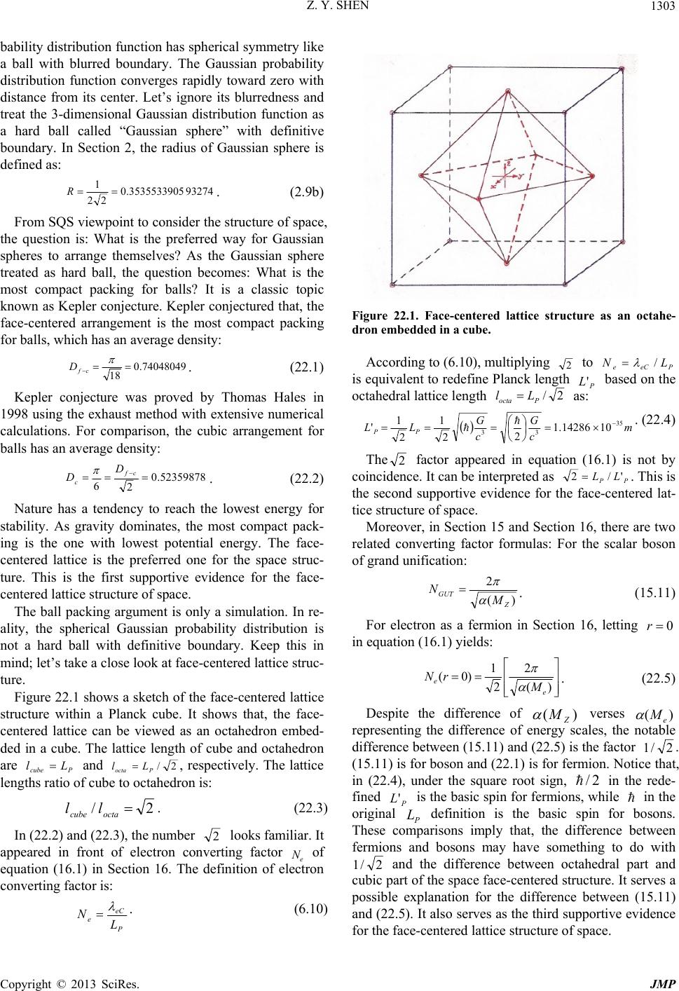

Z. Y. SHEN 1303
bability distribution function has spherical symmetry like
a ball with blurred boundary. The Gaussian probability
distribution function converges rapidly toward zero with
distance from its center. Let’s ignore its blurredness and
treat the 3-dimensional Gaussian distribution function as
a hard ball called “Gaussian sphere” with definitive
boundary. In Section 2, the radius of Gaussian sphere is
defined as:
932743535533905.0
22
1R. (2.9b)
From SQS viewpoint to consider the structure of space,
the question is: What is the preferred way for Gaussian
spheres to arrange themselves? As the Gaussian sphere
treated as hard ball, the question becomes: What is the
most compact packing for balls? It is a classic topic
known as Kepler conjecture. Kepler conjectured that, the
face-centered arrangement is the most compact packing
for balls, which has an average density:
74048049.0
18 


cf
D. (22.1)
Kepler conjecture was proved by Thomas Hales in
1998 using the exhaust method with extensive numerical
calculations. For comparison, the cubic arrangement for
balls has an average density:
52359878.0
2
6 cf
c
D
D

. (22.2)
Nature has a tendency to reach the lowest energy for
stability. As gravity dominates, the most compact pack-
ing is the one with lowest potential energy. The face-
centered lattice is the preferred one for the space struc-
ture. This is the first supportive evidence for the face-
centered lattice structure of space.
The ball packing argument is only a simulation. In re-
ality, the spherical Gaussian probability distribution is
not a hard ball with definitive boundary. Keep this in
mind; let’s take a close look at face-centered lattice struc-
ture.
Figure 22.1 shows a sketch of the face-centered lattice
structure within a Planck cube. It shows that, the face-
centered lattice can be viewed as an octahedron embed-
ded in a cube. The lattice length of cube and octahedron
are Pcube Ll and 2/
Pocta Ll , respectively. The lattice
lengths ratio of cube to octahedron is:
2/
octacube ll . (22.3)
In (22.2) and (22.3), the number 2 looks familiar. It
appeared in front of electron converting factor e
N of
equation (16.1) in Section 16. The definition of electron
converting factor is:
P
eC
eL
N

. (6.10)
Figure 22.1. Face-centered lattice structure as an octahe-
dron embedded in a cube.
According to (6.10), multiplying 2 to PeCe LN /


is equivalent to redefine Planck length P
L' based on the
octahedral lattice length 2/
Pocta Ll  as:
 m
c
G
c
G
LL PP35
33 1014286.1
2
2
1
2
1
' 






  . (22.4)
The 2 factor appeared in equation (16.1) is not by
coincidence. It can be interpreted as PP LL'/2. This is
the second supportive evidence for the face-centered lat-
tice structure of space.
Moreover, in Section 15 and Section 16, there are two
related converting factor formulas: For the scalar boson
of grand unification:
)(
2
Z
GUT M
N


. (15.11)
For electron as a fermion in Section 16, letting 0

r
in equation (16.1) yields:








)(
2
2
1
)0(
e
eM
rN


. (22.5)
Despite the difference of )( Z
M 
verses )( e
M

representing the difference of energy scales, the notable
difference between (15.11) and (22.5) is the factor 2/1 .
(15.11) is for boson and (22.1) is for fermion. Notice that,
in (22.4), under the square root sign, 2/ in the rede-
fined P
L' is the basic spin for fermions, while  in the
original P
L definition is the basic spin for bosons.
These comparisons imply that, the difference between
fermions and bosons may have something to do with
2/1 and the difference between octahedral part and
cubic part of the space face-centered structure. It serves a
possible explanation for the difference between (15.11)
and (22.5). It also serves as the third supportive evidence
for the face-centered lattice structure of space.

Z. Y. SHEN 1304
Postulation 22.1: Space has face-centered lattice
structure as shown in Figure 22.1. It contains two parts:
the cubic part with unit length of P
L and the octahedral
part with unit length of 2/'PP LL .
Explanation: Normalized to P L,
2/12/' PP LL .
According to (2.9b):
22
2
'
22
1PP LL
R . (22.6)
It explains the mathematical reason for the definition
of the radius of Gaussian sphere
R
. In reality, R is
determined by the balance of attractive force and repul-
sive force.
According to Postulation 22.1, space has crystal struc-
ture. It is well known in crystallography that, symmetry
play an important rule to explain crystal properties. Let’s
try to answer the second basic question.
Definition 22.1: In the space with face-centered lattice
structure, symmetry )(rO is defined as a set of vertexes
on the spherical surface centered at an octahedral vertex
with radius
r
; symmetry )(rC is defined as a set of
vertexes on the spherical surface centered at a cubic ver-
tex with radius
r
.
According to Definition 22.1, there are 18 symmetries
for )(rO with 3r and 18 symmetries for )(rC with
3r.
The parameters of 36 symmetries of )(rO and )(rC
with 3r are listed in Table 22.1 and Table 22.2, re-
spectively. In these tables, three sets of numbers are
listed. In the column of “No. of vertexes
TotalCubOct  ..”, “.Oct” and “.Cub ” are the num-
bers of octahedral and cubic vertexes in the symmetry,
respectively. In the column of “No. of equilateral trian-
gles TotalSeparConn  .. ”, “.Conn” and “.Separ ”
are the numbers of connected and separated equilateral
triangles in the symmetry, respectively. In the column of
“No. of squares with center Tota
l
OffOn  ”, “On”
and “Off ” are the numbers of squares with center vertex
of the symmetry on and off the square surface, respec-
tively.
Let’s start from the octahedral part listed in Table 22.1.
)0(O is a basic symmetry represented by a single vertex,
which has a rotational symmetry with any angle. It seems
reasonable to identify )0(O related to the )1(U group.
In the standard model, )1(U represents electromagnetic
interaction mediated by photons. From SQS theory
viewpoint, photon and graviton are two sides of the same
coin. So )0(O is also related to graviton. In fact, the
single vertex of )0(O has dual identity like two sides of
the same coin. It is the vertex on its shrunk sphere sur-
face and it also is the center vertex. It seems reasonable
to identify the former with electromagnetic interaction
and the letter with gravitation. All symmetries have
center vertex not included in Table 22.1 and Table 22.2,
which corresponds to gravity’s universality.
Table 22.1. Symmetries centered at an octahedral vertex in
the face-centered space.
Note: The symmetries marked with * are the 6 essential symmetries.
Table 22.2. Symmetries centered at a cubic vertex in the
face- centered space.
Note: The symmetries marked with *are the 6 essential symmetries.
Symmetry )2/1(O is an important basic symmetry
having 12 vertexes located at following Cartesian coor-
dinates with origin at the center vertex.

Z. Y. SHEN 1305
Cube vertexes:
)
2
1
,
2
1
,0(
1
p, )
2
1
,
2
1
,0(
2

p,)
2
1
,
2
1
,0(
3

p, )
2
1
,
2
1
,0(
4


p;
(22.7a)
Octahedral vertexes:
)0,
2
1
,
2
1
(
5
p)0,
2
1
,
2
1
(
6

p, )0,
2
1
,
2
1
(
7

p, )0,
2
1
,
2
1
(
8

p;
)
2
1
,0,
2
1
(
9
p, )
2
1
,0,
2
1
(
10

p,)
2
1
,0,
2
1
(
11

p,)
2
1
,0,
2
1
(
12


p.
(22.7b)
In which 4 vertexes are cubic type and 8 vertexes are
octahedral type. The hybrid of octahedral and cubic ver-
texes in )2/1(O may serve as a link between fermions
and bosons. The 12 vertexes form 8 connected equilateral
triangles, in which the 4 connected equilateral triangles
in 0x part are shown in Figure 22.2. )2/1(O has 9
squares, in which 3 squares with center vertex on square
surface and the other 6 squares with center vertex off
square surface. The meaning of the equilateral triangles
and the two types of squares will be given later in this
section.
In essence, symmetry )2(O is an enlarged version
of )2/1(O. All symmetries are the same for )2/1(O
and )2(O.The only difference is the linear scale of
)2(O is enlarged by a factor of 2 comparing with
)2/1(O.
Figure 22.2. The vertexes of


2/1O with 4 vertexes lo-
cated at 0x not shown.
)1(O is an important basic symmetry. As shown in
Table 22.1 and Figure 22.3, )1(O has 6 octahedral ver-
texes, The 6 vertexes form an octahedron, which is one
of two parts of the face-centered lattice structure of space
with elongated length scale. The 6 vertexes are paired to
form 3 orthogonal axes with 
90 span angles at center. It
is identified as )3(SO group. )3(SO is closely related
to the )2(SU group. The elements of )3(SO and the
elements of )2(SU are described by three parameters
corresponding to the three Euler angles of a three dimen-
sional rotation. The relation between )3(SO and
)2(SU is that, each rotation in three dimensions of
)3(SO corresponds to two distinct elements of )2(SU .
In some sense, )2(SU is a dual version of )3(SO . It
seems reasonable to relate )1(O with the )2(SU group.
The 6 vertexes of )1(O form 3 squares with center ver-
tex on square surface. A square with center vertex on
square surface is a part of )3(SO and serves as a part of
)2(SU representing weak interaction.
As shown in Table 22.1 and Figure 22.3, )1(O has 8
connected equilateral triangles. The simplest representa-
tion of )3(SU group is a triplet. It seems reasonable to
relate the equilateral triangles in )1(O with )3(SU
triplets such as bgr uuu ,, and bgrddd ,, . SQS the-
ory searching for the )3(SU group comes from a long
way. The first clue came from the 3-dimensional Gaus-
sian probability standard deviation,
 2/1
3. Its
three roots provide one real number and two complex
numbers, which define three axes separated by
120 
on a complex plane as shown in Figure 3.2. The second
clue came from the transportation route of electron mov-
ing in the zigzagging path named “zitterbewegung” hav-
ing 
120 angle with x-axis on a complex plane shown
in Fig. 3.4. The third clue is the fermions’ loop-2 tiny tilt
angle deviated from 
120 
. Now, all these clues
point at one origin, which is the triplet symmetrical
structure in the face-centered lattice. It could serve as the
geometrical foundation for )3(SU group in the real space.
Figure 22.3. The 6 vertexes of

1O.
In essence, the )1()0( OO

is related to three groups
)1(U, )2(SU , )3(SU plus gravitation as the center
vertex, which represent all four types of interactions. As
shown in Section 15, all four types of interactions are

Z. Y. SHEN 1306
united into one. So it should not be a surprise to find out
that, )1()0( OO  related to all four types of interac-
tions.
As shown in Table 22.1, symmetry )3(O has 8 oc-
tahedral vertexes in which 4 of them in 0x region
are shown in Fug. 22.4. The 8 vertexes of )3(O form a
cube, which is one of the two parts of face-centered lat-
tice space structure of space with elongated length scale.
The 8 vertexes of )3(O form 8 connected equilateral
triangles and 6 squares with the center vertex off surface.
Since the )3(SU group has an eight-fold representation,
octet, it seems reasonable to relate )3(O to the
eight-fold. The 6 off center squares represent strong in-
teraction to hold the 8 equilateral triangles representing 8
fermions. A possible physics interpretation is: The octet
of )3(O represents the baryons octet as shown in Fig.
22.5. It includes 8 baryons:)( uudp , )(ddun , )(uus

,
)( dds

, )(
0uss, )( dss 
, )(
0uds, )(uds, in
which each baryon is made of 3 quarks in the first and
second generations.
Figure 22.4. The vertexes of


3O with 4 vertexes located
at 0x not shown.
There is a difference between two different types of
squares. The squares with center vertex on square surface
such as those in )1(O are related to part of )2(SU
representing weak interaction. The squares with center
vertex off square surface such as those in )3(O are
related to a part of )3(SU representing strong interac-
tion. The ratio of center to square distance
D
over
square edge
E
is defined as EDR ED /
/.
For squares with center vertex on surface:
0
/
E
D
RED . (22.8a)
For the squares with center vertex off surface:
0
/
E
D
RED . (22.8b)
Figure 22.5. The baryons octet represented by


3O.
Back to the )2/1(O symmetry, it has 3 squares with
center vertex on surface and 6 squares with center vertex
off surface. It seems that, both weak interaction and
strong interaction are involved with its 8 equilateral tri-
angles. A possible physics interpretation is: )2/1(O
represents 8 fermions, r
u, g
u, b
u, r
d, g
d, b
d, e,
e

and their anti-particles of the first generation. The
weak interactions among 8 fermions represented by 3
squares with center vertex on surface are understandable.
The strong interactions among 6 quarks represented by
squares with center vertex off surface are also under-
standable. But there are squares with center vertex off
surface connecting to equilateral triangles representing
leptons and quarks. What does such type connection
mean?
Figure 22.6 shows the “Symmetries Family Tree” for
)(rO symmetries. It includes all 18 octahedral symme-
tries with radius 3

r. Symmetries are illustrated by
squares with names. The vertical location of the square is
raised according to increasing
r
values of )(rO . Inside
the square from top down, the numbers in three rows,
TotalCubOct


.. , TotalSeparConn 

.. , TotalOffOn


are cited from Table 22.1. In Figure 22.6, there are three
types of connecting lines: A vertical single solid line in-
dicates that the connected two squares have the same
type symmetry with different scales. The forked solid
lines indicate that the top symmetry is a combination of
two symmetries below. The dashed line indicates that the
two connected symmetries are somehow correlated.
In Table 22.1 and Fig. 22.6, the 6 symmetries marked
with * belong to the essential type. In which, )0(O,
)1(O)2/1(O are basic symmetries as mentioned pre-
viously. The other three, )2/3(O, )2/7(O,
)2/13(O, are the lowest symmetries having vertex
numbers 24, 48, 72, respectively.

Z. Y. SHEN 1307
Figure 22.6. The symmetries family tree for

 rO with
3r.
As shown in Table 22.1, Fig. 22.6 and Fig. 22.7,
symmetry )2/3(O is the lowest one has 24 vertexes.
The 24 vertexes of )2/3(O form 8 separated equilat-
eral triangles and 18 squares all with center vertex off
surface, which indicate that the 8 triplets interact to each
other via strong interactions.
Figure 22.7. The vertexes of


2/3O with 12 vertexes lo-
cated at 0x not shown.
As shown in Table 22.1, Figure 22.6 and Figure 22.8,
symmetry )2/7(O is the lowest one has 48 vertexes.
In )2/7(O, the 48 vertexes form 36 squares all with
center vertex off surface and no equilateral triangle.
Figure 22.8. The vertexes distribution of


2/7O.
As shown in Table 22.1, Figure 22.6 and Figure 22.9,
symmetry )2/13(O is the one has most vertexes for
3

r. The 72 vertexes of )2/13(O form 54 squares,
in which 6 squares are with center vertex on surface and
48 squares are with center vertex off surface. )2/13(O
has no equilateral triangle. In the Elementary Particle
Table, the total number of elementary particles is 72,
which is relate to the vertex number 72 of )2/13(O.
Figure 22.9: The vertexes distribution of


2/13O.

Z. Y. SHEN 1308
In the Symmetries Family Tree shown by Fig. 22.6,
there are five columns; the vertical line connections in-
dicate their heritage, which is originated from the bottom
symmetry of each column. Out of five, two columns are
significant. The one called “interactions column” is made
of )0(O, )1(O, )2(Oand )3(O; The other one called
“basic Fermions column” is made of )2/1(O, )2(O
and )8(O.
The foundation of the interactions column is the )0(O
symmetry representing electromagnetic interaction and
gravitation as mentioned previously. As shown in Sec-
tion 15, all interactions are finally unified to gravitation.
The )0(O deserves to be the foundation of interactions
column. From the foundation up, the next symmetry is
)1(O. As mentioned previously, )1()0(OO  represents
gravitation, electromagnetic, weak, and strong interac-
tions. Fig. 22.6 clearly shows that, all four types of in-
teraction are in this column. Up further, there are two
more symmetries, )2(O, )3(O. In which )2(O is an
enlarged version of )1(O. As shown by the forked line,
)2/3()2()3(OOO  , the combination nature of
)3(O is due to the fact that, its radius 3r is suffi-
ciently large to accommodate the additional 24 vertexes
in the enlarged version of )2/3(O. But the core of
)3(O is an enlarged version of )1(O.
Overall, )1(O, )2(O, and )3(O are the interaction
symmetries for the 1st, 2
nd, and 3rd generations, respec-
tively. It implies that, the radius values, 1, 2, 3 are related
to the orders of three generations. )0(O is related to all
symmetries corresponding to gravity’s universality,
which was mentioned previously from another perspec-
tive.
The foundation of basic fermions column is )2/1(O,
as mentioned previously, )2/1(O are related to the
first generation 8 fermions of r u, g
u, b
u, r
d, g
d,
b
d,e, e

and their anti-particles. Since 12/10  ,
12/10  , 221 , and 382  , it seems natural
to relate )2(O to the second generation 8 fermions of
r
s, g
s, b
s, r
c, g
c, b
c,

,


and their
anti-particles; to relate )8(O to the third generation 8
fermions of r
b, g
b, b b, r
t, g
t, b
t,

,


and
their anti-particles. The arrangement confirms the corre-
lation between the values of
r
and the orders of gen-
erations.
The column made of )2/3(O, )2/11(O and
)6(O is based on )2/3(O. )2/11(O and )6(O
have similar properties as )2/3(O. They all have the
same vertexes number 24, the same structure of 8 sepa-
rate equilateral triangles and 18 squares with center ver-
tex off surface.
The column made of )2/5(O and )5(O is based
on )2/5(O. They all have 24 vertexes, and 18 squares
in which 6 with center vertex on and 12 off surface. They
have no equilateral triangle.
The column made of )2/7(O and )2/15(O are
based on )2/7(O. They all have 48 vertexes, 36
squares with center vertex off surface. They also have no
equilateral triangle.
The three columns based on )2/3(O, )2/5(O,
)2/7(O with foundations all start from the second gen-
eration. As shown in Fig.22.6, the columns based on
)2/3(O, )2/5(O, and )2/7(O have 2, 1, and 1
symmetries in the third generation, respectively.
The equilateral triangle and the square are two basic
elements of the face-centered space lattice. The symme-
tries in columns based on )2/5(O, )2/7(O and
symmetry )2/13(O have no equilateral triangle. But
the symmetry with a definitive radius is not alone. The
eighteen symmetries in the Symmetries Family Tree live
together as a family. From family perspective, more
equilateral triangles can be found. For instance, in the
combined symmetry )2/5()2/3(OO  as shown in
Fig. 22.10, besides the 8 equilateral triangles of
)2/3(O, the combination adds 32 more equilateral tri-
angles. )2/5()2/3(OO as a whole has 40 equi-
lateral triangles. The same is true for some other symme-
try. For instance, the combined symmetries of
)5()2(OO , )2/7()2/3( OO ,)2/13()2/11( OO 
and )2/15()2/9(OO all add 8 more equilateral
triangles. The numbers listed in Table 22.1 and Table
22.2 only count the equilateral triangles for each symme-
try alone. Actually, the total number of equilateral trian-
gles in )(rO and )(rC for 3r as two families are
far more than the listed grand total of 224112112

.
Figure 22.10. Additional equilateral triangles of




2/52/3 OO .

Z. Y. SHEN 1309
The symmetries of )(rC centered at cubic vertex have
the same type of symmetries as )(rO . In fact, an )(rO
shifting its center along two orthogonal directions by
2/
P
L for each direction become a )( rC and vice versa.
)(rC ,)(rO have the same “Tota
l
SeparConn .. ” and
“TotalOffOn ”. The difference is that, in the
“TotalCubOct  .. ”column, the numbers of “.Oct ” and
“.Cub ” vertexes may change for )(rC from those of
)(rO and keep the number of “Total ” unchanged.
Therefore, the Family Tree for )(rC is the same type for
)(rO except the two numbers difference in the
“TotalCubOct  .. ”.
The real difference between )( rC and )(rO is their
physics interpretations. As mentioned previously, )(rO
based on the octahedral part is related to fermions and
)(rC based on the cubic part is related to bosons. This
may provide a clue for the physics interpretation of )( rC
symmetries. For instance, the “basic fermions column” of
)2/1(O, )2(O, )8(O is interpreted to represent the
basic fermions of three generations. Likewise, the col-
umn of )2/1(C, )2(C, )8(C is the “basic bosons
column” of three generations. The )2/1(C are related
to g, 1
g, 2 g, 3
g, 4
g, 5
g,

, 1
U of the first gen-
eration bosons. The )2(C are related to 6
g, 7
g, 8 g,
1
G, 2
G, 3
G,
X
, 2
U of the second generation bosons.
The )8(C are related to 4
G, 5 G, 6
G, 7
G, 8 G,
Z
,
W
, 3
U of the third generation bosons. As )3(O is
related to the baryons octet, likewise )3(C is related to
the mesons octet of )( suK,)(
0sdK, )(du 

,
)(ud


,)(
0dsK ,)( usK,


2/)(
0uudd 

,


2/)(
0uudd 

as shown in Figure 22.11.
Figure 22.11. The mesons octet represented by


3C.
In the )(rC system, there are also 6 essential symme-
tries: )0(C, )2/1(C , )1(C, )2/3(C, )2/7(C and
)2/13(C, in which )0(C, )2/1(C , )1(C are basic
symmetries.
Notice that, in Table 22.1 and Table 22.2, the number
163 is total number of vertexes in the 6 essential symme-
tries of )(rO as well as the 6 essential symmetries of
)( rC: 7248241261163  .
In number theory, the number 163 has very special
properties [18].
1) Number 163 is a prime number.
2) Number 163 is the number of columns in the Mon-
ster group’s character table to give the independent
mini-j-functions.
3) Number 163 is related to an irrational number very
close to an integer:
 99259999999999.407687432625374126
163 
e(22.9)
4) It was noticed by Euler that, the number 163 is in
the solutions of an equation: 041)( 2 xxxf
with solutions:
2
1631 i
x . (22.10)
The values of 41)( 2 xxxf for 401

x give
prime numbers.
Moreover, as shown by Fig. 22.12, the Number Tower,
163 is intrinsically related to the m-parameters of the first
generation particles including 7 elementary fermions e,
r
u, g u, b u, r
d, g d, b d and 7 elementary bosons,

,
g
, 1
g, 2 g, 3 g, 4 g, 5 g.
Figure 22.12. The number tower.
The number of vertexes in the 6 essential symmetries
in )(rO system or )(rC system equals to a very special
number of 163 sitting on top of the Number Tower. It has
important implications.

Z. Y. SHEN 1310
1) The set of 6 essential symmetries is not an arbitrary
selection. It is based on mathematics.
2) The total number of elementary particles is 72. It is
the number of vertexes in )2/13(O or )2/13(C. It
also is the largest vertexes number in any symmetry of
)(rO or )( rC with radius 3r. The number 72
close relation with the magic number 163 is based on
mathematics shown by the Number Tower. The SQS
theory Elementary Particle Table given in Section 18 is
based on mathematics.
3) It contains 72 elementary particles including 24 par-
ticles, 24 anti-particles, 24 neutral particles. Notice that,
24, 48 = 24 + 24, 72 = 48 + 24 are the number of ver-
texes for )2/3(O, )2/7(O, )2/13(O and their
counterparts in the )(rC system, respectively.
4) There are only three generations of elementary par-
ticles. It was supported by Prime Number Postulation in
Section 11 and Conclusion 12.1 in Section 12, which are
based on the prime numbers property in number theory.
Here we have the second independent support from
number theory and space symmetry. As the number 72
backed by the magic number 163, there is no room left
for more generation beyond the existing three genera-
tions. Otherwise, the total number of elementary particles
would exceed 72, which is not supported by the Number
Tower and the magic number 163 sitting on top of it.
5) As shown in the Number Tower, the first generation
is the base of all three generations. This is also supported
by the two basic columns in the Symmetries Family Tree,
in which the first generation particles and interactions
serve as the foundations. The second and the third gen-
erations are the extensions of the first generation. This is
also supported by Standard Model. SQS theory provides
the mathematic interpretations based on number theory
and symmetries of space.
According to the above discussion, the 18 + 18 = 36
)(rO and )(rC symmetries with radius 3r cover all
elementary particles and interactions for three genera-
tions. What about the symmetries with radius 3r? The
answer will be given in Section 24.
Ideally, symmetries )(rO , )( rC all are perfect. In re-
ality, the physics groups corresponding to )( rO, )(rC
are not perfect caused by symmetry broken for particles
to obtain mass. Take )2/1(O as an example. In its
perfect symmetry form, the 8 fermions r
u, g
u, b u,
r
d, g d, b d, e, e

all are mass-less to start with.
Each of them obtains mass by broken symmetry in dif-
ferent ways.
The 12 vertexes of )2/1(Oare shown in Fig.22.13.
Equilateral triangle 1171 ppp representing electron in-
cludes a cubic vertex 1
p and two octahedral vertexes
7
p, 11 p. There are three squares 3421pppp , 7865pppp ,
1112109 ppppwith center vertex on surface representing
weak interaction connect to 1
p, 7
p, 11
p respectively.
There are three squares 7251 pppp , 11391 pppp,
128117 pppp with center vertex off surface representing
strong interaction connect to71 &pp , 111 &pp ,
117 &pp respectively. For electron to obtain mass, the
symmetrical triplet 1171 ppp must break under the con-
ditions: (1) All three squares 7251 pppp , 11391 pppp ,
128117pppp with center vertex off surface must break
because electron has no strong interaction. (2) At least
some of three squares 3421 pppp , 7865 pppp,
1112109 ppppwith center vertex on surface must retain
because electron has weak interaction. There are two
possible scenarios meet these requirements.
Figure 22.13. The two triplets for 
e and e

to demon-
strate the retained symmetries and broken symmetries.
Scenario-1:For an electron alone. Two vertexes 7
p,
11
p shift angles to break the triplet 1171 ppp for elec-
tron to obtain mass. The results are: (1) All three squares
7251pppp, 11391 pppp , 128117 pppp with center vertex
off surface are broken for no strong interaction. (2) One
square 3421 pppp with center vertex on surface retains
for weak interaction.
Scenario-2:For electron and electron anti-neutrino
e

as a matched pair. Equilateral triangle 1064ppp
representing e

includes a cubic vertex 4
p and two
octahedral vertexes 6
p, 10
p. There are three squares
3421pppp, 7865 pppp , 1112109 ppppwith center vertex
on surface representing weak interaction connect to 4
p,
6
p, 10 p respectively. There are three squares 8364 pppp ,
122104 pppp , 95106pppp with center vertex off surface
representing strong interaction connect to 64 &pp,

Z. Y. SHEN 1311
104 &pp , 106 &pp respectively. Two vertexes 1
p, 7
p
shift angles to break the triplet 1171ppp for electron to
obtain mass. At the same time, two vertexes 4
p, 6
p
shift the same angles with opposite directions to break
the triplet 1064ppp for e

to obtain mass. The re-
sults are: (1) All six squares 7251 pppp , 11391pppp,
128117pppp , 8364 pppp , 122104 pppp , 95106pppp with
center vertex off surface are broken for no strong interac-
tion. (2) All three squares 3421pppp, 7865 pppp,
1112109 pppp with center vertex on surface retain for weak
interaction. This scenario shows that, besides their ma-
thematical correlation of n-parameter matching, there is a
geometrical correlation between electron and its an-
ti-neutrino e

.
It is conceivable that, Scenario-2 is for regular type
weak interactions with electron and e

as a matched
pair. Scenario-1 is for rare type weak interactions with
electron acting alone without e

. Since Scenario-1 has
only one square retained with center vertex on surface
and Scenario-2 has all three squares retained with center
vertex on surface, which serve as an explanation for the
rarity of the rare type weak interaction for electron with-
out e

.
The similar scenarios are also valid for e
 &
 and

 &
 which belong to the second and third genera-
tions, respectively.
In Figure 22.13, the other two triplets 1252ppp and
983ppp represent up quarks r
u, g
u, b
u and down
quarks r
d, g d, b d. For them to break symmetries to
obtain mass and keep strong interaction as well as weak
interaction , the way to shift angles is under the condi-
tions: (1) At least some of the six squares 7251 pppp,
11391pppp , 128117 pppp , 8364 pppp , 122104pppp ,
95106 pppp with center off surface must retain for strong
interaction. (2) At least some of three squares 3421 pppp,
7865 pppp , 1112109 pppp with center on surface must
retain for weak interaction. The same requirements are
also valid for triplets representing strange, charm, bottom
and top quarks.
These arrangements show the versatility and richness
of the theory.
In the meantime, the above discussions regarding to
the correlations of the symmetries in )(rO and )(rC
systems to physics groups of elementary particles are
hyperbolic. The real correlations between the symmetries
listed in Table 22.1, Table 22.2 and the particles’ groups
such as )1(U, )2(SU , )3(SU require mathematical
proof and more physical verification. But one thing is
clear. If the face-centered space structure is the real space
to accommodate all elementary particles and interactions,
their symmetry groups must be originated from it.
It is important to point out that, all symmetries in the
face-centered space structure are represented by real
numbers. On the other hand, most of particles’ groups are
represented by complex numbers. This is a major differ-
ence. But the difference is only superficial. So far, SQS
theory hasn’t introduced intrinsic time as a variable yet.
In essence, the intrinsic time can be represented by the
phase angle of complex numbers. Once the intrinsic time
variable is introduced, the major difference between
these two systems will be resolved. In fact, intrinsic time
represented by complex numbers’ phase angle is the key
to understand the relation between symmetries )(rO ,
)(rC with 3

r in space and groups in particle physics.
Postulation 22.2: All elementary particles’ groups are
originated from the symmetries in )(rO and )(rC of
space structure with face-centered lattice.
Explanation: Lack of mathematical proof, this is the
best thing one can offer. Table 22.1, Table 22.2 and the
Symmetries Family Tree are useful for further investiga-
tions on this topic.
From SQS theory viewpoint, the physics groups of ba-
sic fermions and bosons are presented in Fig 22.14.
Quarks with different colors are treated as different par-
ticles. Leptons are presented as trefoil model with three
branches combined. The elementary fermions are repre-
sented by 12 equilateral triangles. The 22 elementary
bosons except

and
g
are represented by 8 equilat-
eral triangles, in which the 6 equilateral triangles are
combined into 2 hexagons.

and
g
are located at the
center of equilateral triangle representing
W
,
Z
,
X
.
Figure 22.14 is useful to identify the correlation between
the symmetries in )(rO , )(rC systems and the groups
in particle physics.
Figure 22.14. Elementary particles organized in groups.
Postulation 22.1 and Postulation 22.2 are here to stay
for SQS theory. Hopefully mathematic proofs and more
physics evidences will follow. In fact, they have supports
already. One is the Gaussian sphere and the Kepler-Hales
theorem. If gravitation dominates in the Planck scale
microscopic space, the face-centered lattice structure

Z. Y. SHEN 1312
along with its symmetries is the only logical choice. The
other is that, )( rO and )( rC symmetries with 3

r
fit physics groups well.
Inherited from the face-centered lattice structure, space
has intrinsic symmetries, which serve as the origin of all
groups of elementary particles. Postulation 22.2 is wait-
ing for proof. From SQS theory standpoint, it is the way
Mother Nature selected.
In essence, space is like a crystal, but the macroscopic
space is not a single crystal. Otherwise, the single crystal
space with face-centered lattice is macroscopically ani-
sotropic with preferred directions. That is impossible.
Because theoretically space cannot be in such highly
organized state with extremely low entropy; experimen-
tally there is no evidence for such macroscopic space
anisotropy. In fact, space is amorphous in large scale
with single-crystal or poly-crystal domains. The system
containing enormous identical Gaussian spheres with
relative weak interactions fits well for the conditions of
grand number phenomena. The number of Gaussian
spheres in a typical domain can be estimated according to
(16.13) as:
G
N11 10~ . (22.11)
In which G is the rank number. The G
N11 10~ Gau-
ssian spheres fit in a volume with length scale of
)22/(10~)( 311 P
G
dom LGL , (22.12a)
For 1G:, mLL Pdom 323 10~10~)1( ,, (22.12b)
For 2G:
mLL Pdom296 10~10~)2( , (22.12c)
For 3G:
mLL Pdom2510 10~10~)3( . (22.12d)
Such amorphous space is isotropic with grainy struc-
tures on top of the Planck scale grainy structure. In the
multi-layer grainy structure, the lowest layer with Gaus-
sian sphere as basic building block is single-crystal or
near single-crystal, which serves as the home for ele-
mentary particles with their interactions. We will come
back to this topic in later sections.
The sum of 3-dimensional Gaussian probability
),,(
3zyxS for the cubic part alone was introduced by
(2.24) with subscript changed for identification:
   









ijk
kji
xyz
zzyyxx
cube ezyxSzyxS 222
),,(),,( 3,3

. (22.13)
The octahedral part lattice can be treated as three Car-
tesian systems with 0.5 shifts along two orthogonal axes.
In such coordinate system, the sum of the 3-dimensional
Gaussian probability of the octahedral part alone is:
 ),5.0,5.0(
3
1
)5.0,,5.0(
3
1
)5.0,5.0,(
3
1
,, 333,3 zyxSzyxSzyxSzyxS oct  . (22.14)
In which, the numerical factor 1/3 is for unitarity.
According to (22.13) and (22.14), the overall sum of
Gaussian probability for the 3-dimensional space with
face-centered lattice structure is:

),5.0,5.0(
4
1
)5.0,,5.0(
4
1
)5.0,5.0,(
4
1
),,(
4
1
,,
33
33,3
zyxSzyxS
zyxSzyxSzyxS cf



.
(22.15)
In (22.15), the first term represents the cubic part and
the other three terms combined represent the octahedral
part. The numerical factor 4/1 for unitarity has a deep
meaning. In a Planck cube with the face-cantered lattice
structure, there are 8 Gaussian spheres centered at 8 cu-
bic vertexes at 8 corners and another 6 Gaussian spheres
centered at 6 octahedral vertexes at 6 face centers. For
the cubic part, the 8 spheres at corners each one sharing
with 8 cubes contribute 1 Gaussian sphere to the Planck
cube. For the octahedral part, the 6 spheres at 6 surface
centers each one sharing with 2 cubes contribute 3 Gaus-
sian spheres to the Planck cube. Therefore, the filling
ratio for cubic part versus octahedral part is 1:3 corre-
sponding to unitarity factors 4
1and
4
1
4
1
4
1
4
13


.
It confirms the reason for selecting the numerical fac-
tor 4/1 for unitarity in (22.15).
Actually formula (22.15) serves as a checkpoint for the
consistency of the face-centered space structure. The
face-centered structure is based on the most compact
packing of Gaussian spheres. A hidden assumption is that,
all Gaussian spheres in the space must be identical. In
terms of profile and size, they are identical evidenced by
 2/1 and )22/(1R for all Gaussian spheres.
The four identical numerical factor 4/1 in (22.15)
proved that, all Gaussian spheres also have the same va-
cuons density. It shows that, no matter where they are
located, all Gaussian spheres have the same profile, the
same size and the same vacuons density. In short, they
are identical. Moreover, the four identical numerical fac-
tors also make the ),,(
,3 zyxS cf symmetry with re-
spect to interchanges of three variables z
y
x
,, , which is
required by the geometrical symmetry of the face- cen-
tered lattice structure. So everything is consistent.
According to Postulation 22.1, space has face-centered
lattice structure, in which the cubic lattice structure
serves as one of its two parts. The sums of probability
data listed in Table 2.2 are based on ),,(
3zyxS of (2.24)
for the cubic lattice structure. For the space with
face-centered lattice structure, the sum of Gaussian
probability formula is (22.15). The calculated sums of
probability data based on (22.15) are listed in Table 22.3.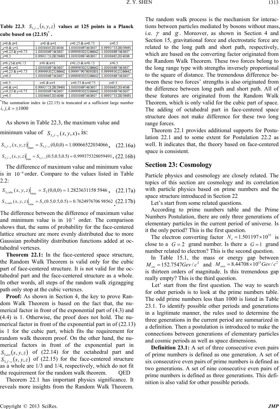

Z. Y. SHEN 1313
Table 22.3:
 zyxS cf ,,
,3  values at 125 points in a Planck
cube based on (22.15)* .
*The summation index in (22.15) is truncated at a sufficient large number
1000,, kji
As shown in Table 22.3, the maximum value and
minimum value of ),,(
,3xyxS cf , is:
40660006652203.1)0,0,0(),,( ,3
max
,3   cfcf SzyxS , (22.16a)
594919993753280.0)5.0,5.0,5.0(),,( ,3
min
,3  cfcf SzyxS . (22.16b)
The difference of maximum value and minimum value
is in 4
10order. Compare to the values listed in Table
2.2:
59462823631158.1)0,0,0(),,( 3
max
,3  SzyxS cube , (22.17a)
985627624976706.0)5.0,5.0,5.0(),,( 3
min
,3 SzyxS cube .(22.17b)
The difference between the difference of maximum value
and minimum value is in 1
10 order. The comparison
shows that, the sums of probability for the face-centered
lattice structure are more evenly distributed due to more
Gaussian probability distribution functions added at oc-
tahedral vertexes.
Theorem 22.1: In the face-centered space structure,
the Random Walk Theorem is valid only for the cubic
part of face-centered structure. It is not valid for the oc-
tahedral part and the face-centered structure as a whole.
In other words, all steps of the random walk zigzagging
path only stop at the cubic vertexes.
Proof: As shown in Section 4, the key to prove Ran-
dom Walk Theorem is based on the fact that, the nu-
merical factor in front of the exponential part of (4.3) and
(4.4) is 1. Otherwise, the proof does not hold. The nu-
merical factor in front of the exponential part in of (22.13)
is 1 for the cubic part, which fits the requirement for
random walk theorem proof. On the other hand, the nu-
merical factors in front of the exponential part in
 zyxS oct ,,
,3 of (22.14) for the octahedral part and


zyxScf ,,
,3 of (22.15) for the face-centered structure
as a whole are 1/3 and 1/4, respectively, which do not fit
the requirement for the random walk theorem. QED
Theorem 22.1 has important physics significance. It
reveals more insights from the Random Walk Theorem.
The random walk process is the mechanism for interac-
tions between particles mediated by bosons without mass,
i.e.

and
g
. Moreover, as shown in Section 4 and
Section 15, gravitational force and electrostatic force are
related to the long path and short path, respectively,
which are based on the converting factor originated from
the Random Walk Theorem. These two forces belong to
the long range type with strengths inversely proportional
to the square of distance. The tremendous difference be-
tween these two forces’ strengths is also originated from
the difference between long path and short path. All of
these features are originated from the Random Walk
Theorem, which is only valid for the cubic part of space.
The adding of octahedral part in face-centered space
structure does not make difference for these two long
range forces.
Theorem 22.1 provides additional supports for Postu-
lation 22.1 and to some extent for Postulation 22.2 as
well. It indicates that, the theory based on face-centered
space is consistent.
Section 23: Cosmology
Particle physics and cosmology are closely related. The
topics of this section are cosmology and its correlation
with particle physics based on prime numbers and the
space structure introduced in Section 22
Let’s start from some related questions.
According to prime numbers table and the Prime
Numbers Postulation, there are only three generations of
elementary particles in the current period of universe. Is
it the only period? This is the first question.
The electron converting factor 23
10501197.1 
e
N is
close to a 2

G grand number. Is there a 1

G grand
number related to electron? This is the second question.
In Table 15.1, the mass or energy gap between
2
/7547.152 cGevMew  and 215/1044708.8 cGevMews 
is thirteen orders of magnitude. Is this tremendous gap
really empty? This is the third question.
Let’ start from the first question. The way to search
for other periods is to look at the prime numbers table.
The odd prime numbers less than 1000 is listed in Table
23.1. To identify possible other periods and generations
in a legitimate manner, the rules used to determine the
three generations in the current period are summarized in
a definition. Then a postulation is introduced to make the
connections between generations of elementary particles
and cosmic periods as well as space dimensions.
Definition 23.1: A set of three consecutive even pairs
of prime numbers is defined as one generation. A set of
six consecutive even pairs of prime numbers is defined as
two generations. A set of nine consecutive even pairs of
prime numbers is defined as three generations. This defi-
nition is also valid for other possible periods.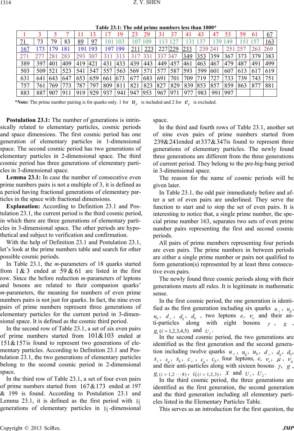

Z. Y. SHEN 1314
Table 23.1: The odd prime numbers less than 1000*
1 3 5 7 11 13 17 1923 2931 3741 4347 53 59 61 67
71 73 79 83 89 97 101 103107 109113 127131 137 139 149 151 157 163
167 173 179 181 191 193 197 199211 223 227 229233239 241251 257 263 269
271 277 281 283 293 307 311 313 317 331337 347349 353359367 373 379 383
389 397 401 409 419 421 431 433439 443449457461463 467479 487 491 499
503 509 521 523 541 547 557 563569571 577 587593599601607 613 617 619
631 641 643 647 653 659 661 673677683691 701 709719 727733 739 743 751
757 761 769 773 787 797 809 811821 823827829839853 857859 863 877 881
883 887 907 911 919 929 937 941947953967971977 983991997
*Note: The prime number pairing is for quarks only. 1 for r u is included and 2 for r e is excluded.
Postulation 23.1: The number of generations is intrin-
sically related to elementary particles, cosmic periods
and space dimensions. The first cosmic period has one
generation of elementary particles in 1-dimensional
space. The second cosmic period has two generations of
elementary particles in 2-dimensional space. The third
cosmic period has three generations of elementary parti-
cles in 3-dimensional space.
Lemma 23.1: In case the number of consecutive even
prime numbers pairs is not a multiple of 3, it is defined as
a period having fractional generations of elementary par-
ticles in the space with fractional dimensions.
Explanation: According to Definition 23.1 and Pos-
tulation 23.1, the current period is the third cosmic period,
in which there are three generations of elementary parti-
cles in 3-dimensional space. The other periods are hypo-
thetical and subject to verification and confirmation.
With the help of Definition 23.1 and Postulation 23.1,
let’s look at the prime numbers table and search for other
possible cosmic periods.
In Table 23.1, the m-parameters of 18 quarks started
from 3&1 ended at 61&59 are listed in the first
row. Since the before reduction m-parameters of leptons
and bosons are related to their companion quarks’
m-parameters, the meaning for numbers of even prime
numbers pairs is not just for quarks. In fact, the nine even
pairs of prime numbers represent three generations of
elementary particles for the current period in 3-dimen-
sional space. It is defined as the cosmic third period.
In the second row of Table 23.1, a set of six even pairs
of prime numbers started from 103&101 ended at
157&151 is found to represent two generations of ele-
mentary particles. According to Definition 23.1 and Pos-
tulation 23.1, the two generations of elementary particles
belong to the second cosmic period in 2-dimensional
space.
In the third row of Table 23.1, a set of four even pairs
of prime numbers started from 173&167 ended at 197
& 199 is found. According to Postulation 23.1 and
Lemma 23.1, it is defined as the first period with 3
1
1
generations of elementary particles in 3
1
1-dimensional
space.
In the third and fourth rows of Table 23.1, another set
of nine even pairs of prime numbers started from
241&239 ended at347&337 is found to represent three
generations of elementary particles. The newly found
three generations are different from the three generations
of current period. They belong to the pre-big-bang period
in 3-dimensional space.
The reason for the name of cosmic periods will be
given later.
In Table 23.1, the odd pair immediately before and af-
ter a set of even pairs are underlined. They serve the
function to start and to stop the set of even pairs. It is
interesting to notice that, a single prime number, the spe-
cial prime number 163, separates two sets of even prime
number pairs representing the first and second cosmic
periods.
All pairs of prime members representing four periods
are even pairs. The prime numbers in between periods
are either a single prime number or pairs not qualified to
form generation(s) represented by at least three consecu-
tive even pairs.
The newly found three cosmic periods along with their
generations meets all rules. It is legitimate in mathematic
sense.
In the first cosmic period, the one generation is identi-
fied as the first generation including six quarks r
u, g u,
b
u, r d, g d, b d , two leptons
e
, e

and their an-
ti-particles along with eight bosons

,
g
,
i
g)5,4,3,2,1(

i and 1
U.
In the second cosmic period, the two generations are
identified as the first generation and the second genera-
tion including twelve quarks r
u, g u, b u, r d, g
d, b
d,
r
s, g
s, b
s, r
c, g
c, b
c, four leptons, e, e

,

,


and their anti-particles along with sixteen bosons

,
g
,
i
g)82,1(




i, i G)3,2,1(

i,
X
and 1
U, 2 U.
In the third cosmic period, the three generations are
identified as the first generation, the second generation
and the third generation including all elementary parti-
cles listed in the Elementary Particles Table.
This serves as an introduction for the first question, the

Z. Y. SHEN 1315
details will be given later.
Let’s turn attention to the second question, which
concerns electron converting factor e
N as 2

G grand
number. In essence, it is to search whether there is an
electron intermediate state in existence corresponding to
1G grand number 11
10~
e
N. Let’s go back to the lo-
gistic equation of (16.1). Substitutinge
N to replace e
N
and )(Z
M

to replace )(e
M

, a numerical calcula-
tion found:
0104048421709430.2)(22 131
)(2
1 
Z rx
eMeN


(23.1)
11
,int 1056858745288094.3  eere NN , (23.2a)
200378771029244.3)125.0()(1


x, (23.2b)
6378494231955224.2r. (23.2c)
The
r
value given by (23.2a) falls into the range of
32 1 r. According to Table 16.1, for
r
value in
this range, the logistic recurrent process oscillates and
converges to:
5873218.0/11  r. (23.3).
This scenario fits the intermediate state well, in which
the logistic recurrent process is in progress and about half
way through toward the threshold.
The
11
int, 1056858745288094.3 ee NNgiven by
(23.2a) is a 1G grand number. The mass of the elec-
tron intermediate state is:
228
int,int, /97323432.4/1097993553.1/cGeVMcGeVNMM MaxePe  .
(23.4)
According to Rule 6.1, it cannot be a standalone fer-
mion state, two intermediate states must appear in pair to
form a scalar boson called “e-boson” with mass be
M,
converting factor be
N and length scale be L:
28
int, /1095987106.32 cGeVMMebe  , (23.5a)
11
int, 109372644.1
2
1

e
be
P
beN
M
M
N, (23.5b)
m
cM
h
L
be
be24
1013110359.3 

 . (23.5c)
Now the second question regarding electron interme-
diate state is answered. The mass of int,e
M and be
M
fall into the middle of the tremendous gap between e
w
M
and ews
M. The gap is not empty. So it answers the third
question as well.
Let’ turn attention to details of the first question.
According to the cosmology standard model, the uni-
verse started from a big bang with extremely high energy
corresponding to extremely high temperature. From SQS
theory perspective, there was a “pre-big-bang period”
represented by a set of 9 prime number even pairs started
from 241&239 and ended at 347&337 found in
Table 23.1 as mentioned previously. The pre-big-bang
universe was a 3-dimensional “overheated liquid state”.
Its details will be given later.
The overheated liquid state is unstable, any random
stimulation causes evaporation. The Gaussian spheres
were evaporated and free to fly as 0-dimensional objects
in space represented by the prime numbers 211, 223, 227,
229, 233 between the two sets of prime number even
pairs representing the pre-big-bang period and the first
period. Let’s call it the “0-period”.
The universe was born at the big bang. The cosmic
time is set to zero: 0
0

t, and the new born universe
started to evolve.
During the 0-period, the flying around Gaussian
spheres attracted each other by gravitational force and
intended to gather as groups, which nurtured the first
period.
The first cosmic period started at time scale 1
t with
length scale 1
L:
mLLLPGUT 33
1101475.1~71 
 , (23.6a)
scLtt GUTGUT 42
1108278.3~/ 
 . (23.6b)
At time 1
t, the first cosmic period started. The flying
Gaussian spheres were gathered and organized into
1-dimensional array in 1-dimensional space.
The 1-dimensional space was built as an array of
Planck scale face-centered cubes. If the building block of
array is a Planck cube centered at a cubic vertex includ-
ing 12 octahedral vertexes, according to Table 22.1 and
Table 22.2, only three symmetries )0(C, )2/1(C,
)0(O are fully effective. There is no fermion in the
three symmetries. This scenario is not acceptable. If the
building block of array is a Planck cube centered at an
octahedral vertex including 4 cubic vertex and 8 octahe-
dral vertexes, according to Table 22.1 and Table 22.2,
three symmetries )0(O, )2/1(O, )0(C are fully
effective. It include 8 first generation fermions r
u, g
u,
b
u, r d, g
d, b
d, e, e

and 8 anti-fermions in
)2/1(O and 2 bosons

,
g
in )0(O responsible for
electromagnetic interaction and gravitation. As shown in
Section 15, the grand unification is to unify electromag-
netic interaction into gravity. In (23.6b), 1 t is derived
from GUT
L originated from GUT M. At time 1
t, the re-
verse process of grand unification happened, electro-
magnetic interaction was separated from gravity. There-
fore, in the first cosmic period after 1 t, the two bosons

,
g
in )0(O showed up is natural and fully ex-
pected.
For the symmetry )1(O representing the other 6 first
generation bosons i
g)5,4,3,2,1(

i and 1 U, out of its 6
vertexes, only 2 of them are in the array counting for one
third of its constituents. It indicates that, 2 out of 5 glu-
ons such as 1
g and 2
g would be in effect. According
to Table 13.2A and 13.2B , in the gluon links among r u,

Z. Y. SHEN 1316
g
u, b
u, 9 of the 12 links are made of 1
g and 2 g; in
the gluon links among r
d, g
d, b
d, 3 of the 6 links are
made of1
g and 2 g. It means that strong interaction is
partially in effect.
Actually, the first cosmic period was in 3
1
1-dimen-
sional space, which is a fractal space. The space dimen-
sion was not fixed, instead, it was a developing process
from 1-dimension gradually toward 2-dimension. Ac-
cordingly, the cross section of the array gradually in-
creases from PP LL11 to PP nLL 1. When the width
number 2n, the symmetry )1(O has 4 out of its 6
vertexes in the wider array. As a result, 2 more gluons
such as 3
g and 4
g would be in effect. According to
Table 13.2A and 13.2B , in the gluon links among r
u,
g
u, b u, all 12 links are made of 1
g, 2 gand 3 g; in
the gluon links among r
d, g
d, b
d, all 6 links are made
of 1
g, 3
g and 4 g. It means that strong interaction for
the first generation quarks is fully in effect.
This scenario looks reasonable and is accepted by SQS
theory.
During the first period and other early cosmic periods,
all particles are in their extremely high energy states cor-
responding to extremely high temperature, which are
quite different from their ordinary states. For instance,
according to Figure 19.1 and Figure 19.2, the gluon links
binding quarks to form proton and neutron all are made
of 1
g, 2 g, 3
g and 4
g. But it does not mean that,
proton, neutron were formed during the first cosmic pe-
riod after the array cross section increased to PP LL 21

.
Because of the extremely high temperature, it was im-
possible to form any hadron. Instead, “quark-antiquark
liquid state” would be formed from these first generation
quarks and anti-quarks bound by strong interaction
mediated by these in effect gluons1
g, 2
g, 3 g and
4
g.
The second cosmic period started at 2 t with length
scale 2
L:
mLLMLL PPsewsew 311
2104678.1~9082)(71~ 



, (23.7a)
stcLt Psew40
2108963.4~9082~/  . (23.7b)
After 2 t, the second cosmic period started and the
space became 2-dimensional, The 2-dimensional space is
a membrane. In order to accommodate major symmetries
of the first and the second generations, the thickness of
membrane should be P
L2. As shown in Table 22.1 and
Table 22.2, the 2-dimensional membrane with P
L2
thickness centered at a cubic vertex accommodates 7
fully effective symmetries )0(C, )2/1(C, )1(C,
)2/3(C, )2(C,)0(O, )2/1(O, which does not in-
clude the second generation fermions. This scenario is
unacceptable. On the other hand, the 2-dimensional
membrane with P
L2 thickness centered at an octahedral
vertex accommodates 7 fully effective symmetries )0(O,
)2/1(O, )1(O, )2/3(O, )2(O, )0(C, )2/1(C,
which include the first generation 8 fermions r
u, g
u,
b
u, r
d, g d, b
d, e, e

and their anti-particles rep-
resented by )2/1(O plus second generation 8 fermions
r
s, g
s, b
s, r
c, g
c, b
c,

,


and their an-
ti-particles represented by )2(O. Symmetry )2(O is
not fully effective. Among its 6 vertexes, only 4 are in-
cluded. The effective bosons for the second period are
the first generation 8 bosons
g
,

, i
g)5,4,3,2,1(

i,
1
U plus second generation 6 bosons corresponding to
two third of 9 bosons plus 1 anti-boson 0
X
in second
generation. The second period started at length scale
sew
LL 

2, which is the characteristic length of elec-
troweak-strong unification. The scalar boson 2
U for
that unification must be included. The strong interaction
was separated and fully effective. All 8 gluons
i
g)8,,2,1(




i must be included. There are two addi-
tional second generation bosons as candidates selected
from the remain second generation bosons: 3 massons
i
G)3,2,1(

i,
X
and anti-boson
X
. Because
X
,
X
cannot be produced without its counterpart, there are
only two possible selections. One is
X
and
X
, the
other is two massons.
The second period include the first and second genera-
tions 16 fermions: r
u, g u, b u, r
d, g
d, b
d, r
s,
g
s, b s, r c, g c, b c, e, e

,

,


and 16
anti-particles along with 12 bosons for sure:
g
,

,
i
g)8,,2,1(




i, 1
U, 2 U, plus 2 additional bosons or 1
boson and 1 anti-boson from one out of two choices. Ei-
ther way sounds reasonable. This scenario is accepted by
SQS theory.
Conclusion 23.1: Weak interactions are not in effect
in the second cosmic period with 2-dimensional space.
Proof: The reason for Conclusion 23.1 is that, the ne-
cessary mediators and intermediate states of weak inter-
actions are not available in the second cosmic period.

W and 0
Z
as third generation gauge bosons are not
available for the second cosmic period according to Pos-
tulation 23.1.
X
and X or two out of three massons
i
G)3,2,1(

i are available depending on the choice. But
the hypothetical gauge bosons
X
and X serving as the
intermediate state for some type of weak interactions
have similar behavior as their counterpart 
W and 0
Z
,
they must have massons’ assistance to make the
m-parameters match and the n-parameters match as well
as to fill the mass gap described in Section 14. Unfortu-
nately, the two choices can only provide either
X
and
X
or two massons but not both. The necessary media-
tors and interstates are not in existence, weak interactions
cannot perform. QED
Conclusion 23.1 is important. It leads to a prediction
given later.
In the second comic period, all second generation par-
ticles except perhaps


and


are unstable. Under
normal conditions, they are subject to decay via weak

Z. Y. SHEN 1317
interactions. But the second cosmic period did not pro-
vide normal conditions, in which things turned out quite
differently. According to Conclusion 23.1, weak interac-
tions are not in effect in second cosmic period. The un-
stable particles in the 2-dimensional membrane cannot
decay via weak interactions. They must hold until the
third period, when the gauge bosons 
W, 0
Z
, 0
X
and
massons are effective, then decay in the 3-dimensional
space. Moreover, the big bang produced equal amount of
elementary particle and anti-particles. Some of them
remained in the second period. Whether they had the
chance to annihilate in second cosmic period is an inter-
esting question, which will be discussed later.
The third period started at 3
t with length scale
be
LL  
3 of (23.5c):
mLLL Pbe2411
3101311.3109373.1  , (23.8a)
scLt 32
33 100444.1/ 
 . (23.8b)
After 3
t, the space became 3-dimensional. All parti-
cles listed in the Elementary Particle Table showed up.
All symmetries listed in Table 22.1 and Table 22.2
became fully effective. All four types of interactions
were into full play. In fact, it is the universe started at
13.7 billion years ago we living in now.
The transition from the 2-dimensional space to the
3-dimensional space was a phase transition, which trig-
gered the cosmic inflation.
The e-boson played a pivotal role in the cosmic infla-
tion. It sets the length scale 3
L and time scales 3
t of
the cosmic inflation. In addition, the logistic recurrent
processes started at time 1 t, they reached about halfway
at 3
t, which corresponds to the birth of the e-boson.
More importantly, the scalar e-boson with mass of
GeVM bs 8 109599.3 
 acted as the inflaton. Accord-
ing to the cosmology standard model, during the rapid
expansion period, the inflation was driven by a scalar
boson called inflaton. Physicists are looking for the
inflaton for some time without satisfaction. Here is the
e-boson. It is a scalar boson; it is heavy and relatively
stable. More importantly, it was born at the very begin-
ning of the cosmic inflation and drove the space expan-
sion to the very end of the inflation. Then it continued its
journey toward the Compton scale and become a pair of
ordinary electron and positron. The e-boson is not tailor
made for the cosmic inflation; instead, it is the require-
ment of logistic process, grand number, and Rule 6.1. In
short, the e-boson fits the inflaton perfectly.
The time scale of st32
3100444.1~
 is roughly agreed
with the time of the cosmic inflation proposed by cos-
mology standard model. It is a good thing, but it raises
questions. If 3 t corresponds the time of the cosmic in-
flation, what about 1 tand 2
t? Were there two more
inflations before the big one? These are very interesting
questions. Space dimensions change is equivalent to
phase transition, which releases energy causing inflation.
The scale of inflation is determined by the amount of
released energy. In this case, the released energy depends
on three factors: the number of Planck cubes involved,
the contraction depth of space elements, the total energy
involved. The numbers of Planck cubes involved are 71,
9082, and 232
int,100048.6)2( e
N for the phase transi-
tions occurred at 1
t, 2 t, and 3 t, respectively. The ra-
tios of contraction depth are estimated as
1~)71(~ 1/0
1
R, 95~)9082(~ 2/1
2
R,153/223
3101176.7~)100048.6(~ R
for the transitions occurred at 1
t, 2 t and 3
t, respec-
tively. If the potential energy released is proportional to
the square of )3,2,1(,iRi, The ratios for the released
energy is estimated as
312
3
2
2
2
110066.5:9082:1~:: RRR ,
for the phase transitions occurred at 1
t, 2 t and 3
t,
respectively. In terms of scales, it seems no comparison
between the two inflations occurred at 1
t, 2 t and the
big one at 3
t. The two inflations at 1 t, 2 t were just
mini rehearsals of the big show at 3
t. But there is an-
other factor involved. According to the energy conserva-
tion law, the total energy of three cosmic periods and the
0-period should be the same. The big difference in the
numbers of Planck cubes involved is partially compen-
sated by energy per Planck cube. It makes the released
energy of three inflations quite different from
312
3
2
2
2
110066.5:9082:1~:: RRR . According to this
argument, the difference of three inflations’ scales could
be closer. In other words, there were two comparable
scale rehearsals before the big show.
But the three inflations scenario has a glitch. Phase
transition is an abrupt event occurred in an extremely
short time interval. Noticed that, the 1-dimensional space
actually is 3
1
1-dimensional, which has fractal behaviors.
The transition from 3
1
1-dimensional space to
2-dimensional space is not necessarily corresponding to a
violent phase transition happened suddenly at 2 t. In-
stead, it could be a gradual process. If this argument
holds, there were only two cosmic inflations occurred at
1
t and 3
t.
According to SQS theory, the phase transition hap-
pened at 3 t corresponds to the big cosmic inflation
proposed by cosmologist Ruth [19], which has been veri-
fied by astronomy observations. According to SQS the-
ory, there is at least one more phase transition happened
at 1 t corresponding to a cosmic inflation before the big
one happened at 3
t. It should also leave some footprints
somewhere. The most like place is the cosmic microwave
background radiation (MBR).
From SQS theory perspective, the early cosmological
history is the natural evolution of the space structure with
Gaussian spheres as building blocks. The results derived

Z. Y. SHEN 1318
from it fit the cosmology standard model pretty well.
SQS theory contributions are: (1) The cosmic periods
and the generations of elementary particles are correlated
to space dimensions; (2) It is determined by the prime
numbers. In essence, everything is traced back to ma-
thematics.
Astronomical observations and measurements such as
gravity lens effect and the cosmic MBR have found the
evidence for dark matter. Astrophysics observations in-
dicate that, the composition of universe is approximately
5% visible matter, 21% dark matter and 74% dark energy.
What is dark matter made of? Physicists are looking for
the answer for quite some time. The favorite candidates
for dark matters are hypothetical particles such as axion
and neutrarino etc. These dark matter candidates are hy-
pothetic elementary particles and only interact with visi-
ble matter via gravitation and weak interaction. Around
the world, many underground experiments have been
carried out to detect dark matter candidate particles rare
interaction with visible matters. Despite the extensive
efforts, so far, there is no confirmed positive result. It is
the time for a second thought.
Let’s look at the dark matter issue from SQS theory
perspective. The Elementary Particle Table includes sev-
eral undiscovered neutral heavy particles: i
G,
)8,2,1( i,
X
, 1
U, 2 U, 3 U. But perhaps all of them
are unstable particles, which do not fit the requirements
for the dark matter. On the other hand, notice that, the
reliable evidences for the existence of dark matter all are
based on its gravitational effects. The idea for dark mat-
ter as elementary particle having weak interaction with
visible matters is hypothetical without experimental
support. There is no reason to reject other types of dark
matter candidates interacting with visible matters only
via gravity. Moreover, there is no reason to reject radical
ideas such as: dark matter is made of something other
than undiscovered elementary particles.
Hypothesis 23.1: At least part of dark matters in the
universe is the debris left over from the cosmos inflation.
The dominate part of this type dark matters is 2-dimen-
sional membranes, which interact with visible matters
only via gravity.
Explanation: The cosmos inflation was a gigantic
violent event happened in an extremely short time inter-
val with tremendous amount of energy involved. It is
inconceivable to assume that, the phase transition only
produced the 3-dimensional space out from a 2-dimen-
sional membrane. It is more natural to conceive that, the
phase transition produced the 3-dimensional space along
with many pieces of debris. Since the pre-state of phase
transition is a 2-dimensional membrane, the dominate
part of debris is relatively small pieces of 2-dimensional
membrane. The phrase “part of dark matters” in Hy-
pothesis 23.1 leaves room for other possible dark matter
candidates.
We haven’t found any dark matter, because we were
looking for the wrong candidates. Dark matter may not
be undiscovered elementary particles. According to Hy-
pothesis 23.1, dark matters are left over debris from the
comic inflation and most of them are 2-dimentional
membranes flooding around in 3-dimentional space.
The new type experiments for searching dark matter
should be based on its gravitation effects. Astronomical
observations have found that, dark matter is mixed with
visible matter all over the universe. Therefore, it is pos-
sible to design experiments for searching dark matter
based on its gravitational effects.
Suggestion 23.1: The new type of experiments for
searching dark matter is to use extremely sensitive gravi-
tation meter isolated from earthly interferences. As earth
rotating around the sun, occasionally, a piece of 2-dimen-
sional membrane passes through the meter, which will
produce a signal to indicate its gravitational effect as the
evidence of its existence. The signal can be recorded by
monitoring apparatus and analyzed by computer with re-
cognition software.
There is another possibility to verify dark matter. A
piece of relatively large 2-dimensional membrane is ca-
pable to attract other membranes via gravity. When suf-
ficient membranes get together in the right way, it is pos-
sible to trigger a mini-inflation type of phase transition to
transfer a piece of 2-dimensional dark mater into a chunk
of 3-dimentional visible matter. From our perspective,
the event is like that, a chunk of 3-dimensional visible
mater suddenly appears from void. According to Conclu-
sion 23.1, in the 2-dimensional membrane weak interac-
tions are not in effect. The second generation unstable
elementary particles such as muon, hadrons made of
s-quarks, c-quarks and their anti-articles in the membrane
hold their decay and wait for the chance. Immediately
after the mini-inflation, in the new born 3-dimensional
chunk, gauge bosons
W
,
Z
,
X
and massons become
readily available and fully effective. These unstable par-
ticles are eligible to decay. As a result, a shower of high
energy particles is released, which can be detected and
serve as the evidence of the mini-inflation and dark mat-
ter. In addition, as mention previously, there were parti-
cles and anti-particles left in the 2-dimensional mem-
brane. If they did not have a chance to annihilate in the
membrane, these particles and anti-particles should re-
lease at once at the mini-inflation. If they were annihi-
lated in the membrane already, the annihilation products
remained in the membrane should release also. Either
way, showers of high energy

-rays and other particles
and anti-particles should be detectable.
Suggestion 23.2: The way to verify the mini-inflation
is to monitor the primary high energy cosmic rays. If the
components fit the pattern of decay modes branching

Z. Y. SHEN 1319
ratios of the second generation unstable particles or their
annihilations products, these events serve as the evidence
for the mini-inflation as well as for dark matter.
Explanation: In fact, occasionally cosmic rays with
extremely high energy has been observed coming from
places such as the center of galaxy. If the branching ra-
tios and products fit the right pattern, they can serve as
the evidence of mini-inflation and dark matter. The key
is to analyze the components whether fits the right pat-
tern or not.
So far, the cosmic history from big bang through infla-
tion up to the current period is explained pretty well
based on the prime numbers even pairs listed in Table
23.1 and the space structure and symmetries described in
Section 22. It is natural to ask: What is the pre-big-bang
history? What is the outlook for the cosmic future? The
answers are also in the prime numbers table.
As mentioned previously, in the third row and fourth
row of Table 23.1, there is another set of 9 even pairs
starting from 241&239 and ended at 347&337 . Ac-
cording to Definition 23.1, it is qualified to be a
3-dimensional space corresponding to the pre-big-bang
period. Its m-parameters are much larger than those of
current 3-dimensional universe. It indicates that the ele-
mentary particles in the pre-big-bang period had ex-
tremely high energy to form the overheated quark- anti-
quark liquid state. More details will be given in Section
24.
Now let’s look at the future destiny of universe. The
cosmic history from pre-big-bang period through the
0-period, first period, second period and the current third
period indicate that, in the cosmic scale, the direction of
time arrow is from the set with larger prime numbers
toward the set with smaller prime numbers. It means that,
to read the sets of prime numbers listed in Table 23.1
corresponding to cosmic history should be from bottom
up and from right to left. In other words, the cosmic time
sequence is from the period with the set of larger prime
numbers to the period with the set of smaller ones.
Now we are in the current third period corresponding
to a set of 18 + 1 = 19 prime numbers, in which 18 prime
numbers for quarks is listed in the first row of Table 23.1
plus the even prime number 2 for electron not listed. In
the set of 19 prime numbers, the smallest one is 1. At
first glance, it seems no prime number smaller than 1. If
that is the case, our universe eventually will come to an
end. But Mother Nature always has her ways. The num-
ber axis centered at 0 has two wings, the right wing
points toward positive numbers and the left wing points
toward negative numbers. There is a set of negative
prime numbers, which is exactly the same as ordinary
prime numbers set with minus signs. Taking the negative
prime numbers into account, there is a future for our un-
iverse.
Definition 23.2: The negative prime numbers are de-
fined as the negative value of the ordinary prime num-
bers, which correspond to the prime numbers listed in
Table 23.1 with minus signs.
Hypothesis 23.2: In terms of cosmology and elemen-
tary particles, the negative prime numbers act the same
way as their positive counterparts except that, all parti-
cle’s m-parameters and n-parameters change signs.
Definition 23.2 and Hypothesis 23.2 lay the theoretical
foundation for the future and the pre-big-bang history of
the universe.
Astronomical observations found that, the universe
currently is expanding with accelerating speed caused by
the repulsive force of dark energy. Some cosmic models
predicted that, the expansion will slow down and eventu-
ally turn to contraction. The contracting universe re-
verses its expansion process and finally back to a big
crunch corresponding to the reverse of the big bang.
Then the whole thing starts over again. The model is call-
ed “oscillation model”. The universe cycles by itself over
and over. Hypothesis 23.2 supports the oscillation model
based on the negative prime numbers. The following is
the scenario of universe future from SQS theory perspec-
tive based on Hypothesis 23.2.
The expansion of universe will slow down due to the
dilution of dark energy density and eventually turn into a
contraction. The evidence is in the extended prime num-
bers table. As time passing by, the corresponding prime
numbers become smaller. Finally it reaches 1, which is
marked as the end of the current third period. But the
cosmic evolution does not stop. It continues its journey.
The number passes through 0, which is the m-parameter
for the graviton. Then it enters into the negative territory.
According to Hypothesis 23.2, the negative prime num-
bers correspond to the m-parameter changing sign.
Theoretically, here are two ways for the n-parameter to
react: (1) The corresponding n-parameters also change its
sign; (2) The corresponding n-parameters do not change
sign. According to Definition 11.2, the second way
means that all particles become anti-particles. All matters
in the universe suddenly become anti-matters! This sce-
nario is impossible. Then the only possibility is the first
way as Hypothesis 23.2 stated. The simultaneously
changing signs of both m-parameter and n-parameter
indicate that, all particles change their handedness corre-
sponding to change the direction of their momentum.
This scenario is supported mathematically and physically.
The mathematic support comes from prime numbers. At
the time universe stop expansion, the prime number se-
quence passes 0 and enters the negative territory causing
m-parameters and n-parameters both changing their signs.
The physical support is that, as universe stops expansion
and starts to contract corresponding to all particles’ mo-
mentum changing direction. This scenario is much easy

Z. Y. SHEN 1320
to be accepted than the other scenario, all particles sud-
denly become anti-particles.
Sine the negative prime numbers table is the same as
the positive prime number table except the minus signs,
as the universe starts to contract, it basically follow the
reversed process of the expansion universe. It is like to
play a video in the reverse order. The consecutive cosmic
events sequence is like that, as the negative third period
coming to its end, the universe enters to the negative
second period, then the negative first period, the negative
0-period, the negative big bang, i.e. the big crunch, fi-
nally reaches the negative pre-big-bang period, i.e. the
post-big-crunch period, One cycle of universe oscillation
is completed. The post-big-crunch period is the same as
pre-big-bang period except that all m-parameters and all
n-parameters change signs corresponding to time arrow
in the opposite direction. To start the next cycle, the post-
big-crunch period must transfer into the pre-big-bang
period. This process can be realized through a “time tun-
nel”. Since both periods possess extremely high energy,
according to general relativity, the space-time is extre-
mely curved providing the conditions to form time tunnel.
Figure 23.1 shows a diagram to illustrate the evolution of
the cyclic universe.
Figure 23.1. Illustration of cosmic cycle based on prime
numbers.
The repetitive cycles of oscillation model are in the
cosmological sense. It does not mean that, everything in
the universe will repeat exactly. In fact, according to
SQS theory, space is stochastic in nature, which prohibits
absolute determinism at the fundamental level and upper
levels.
The cosmic history described in this section is based
on the prime numbers table and the Prime Number Pos-
tulation. It especially depends on the discovery of three
sets of consecutive prime number even pairs serving as
the mathematical bases for the first period, the second
period and the pre-big-bang period. The correspondence
of the original set of 18+1 prime numbers to the current
third period is supported by many evidences. The ques-
tion is: What is the mathematic relation between the
newly found three sets of prime numbers and the original
set of 18+1 prime numbers?
Let’s start from the first prime numbers of the three
sets, according to Table 23.1, which are 167, 101, and
239 for the first, second, and per-big-bang period, re-
spectively. A simple arithmetical calculation found the
following formulas.
Period-I:
)321(3129231917131175321167











,
(23.9a)
Period-II:
231917131175321101








, (23.9b)
Period-III*:
41373129231917131175321239











.
(23.9c)
In which, Period-I, Period-II, and Period-III* are
marked for first period, second period and pre-gig-bang-
period, respectively.
It is interesting to find some rules in (23.9).
1) The first prime number 101 corresponding to Pe-
riod-II equals to the sum of the ten consecutive prime
numbers from 1 to 23 in the set of 18+1 prime numbers
for the current third period.
2) The first prime number 239 corresponding to Pe-
riod-III* equals to the sum of the fourteen consecutive
prime numbers from 1 to 41 in the set of 18+1 prime
numbers for the current third period.
3) The first prime number 167 corresponding to Pe-
riod-I equals to the sum of the twelve consecutive prime
numbers from 1 to 31 plus (1 + 2 + 3) in the set of 18+1
prime numbers for the current third period. The repeat of
three prime numbers (1 + 2 + 3) represents the fact that
the space of Period-I is 3
1
1-dimensional, which is dif-
ferent from Period-II and Period-III*.
The last prime numbers of the three sets corresponding
to period-I, period-II, and period-III* are, 199, 157, 347,
respectively.
Period-I:
)321()7()13(535961199 




, (23.10a)
Period-II:
)37(5961157



, (23.10b)
Period-III*:
)43(414347535961347 




. (23.10c)
There are also some rules in (23.10).

Z. Y. SHEN 1321
1) The order of summation in (23.10) is backwards
from the last prime number 61 of the 18 + 1 prime num-
bers set and consecutively takes the next one.
2) After the backwards consecutive summation ended,
it jumps to the prime number(s) shown in parenthesis.
3) For Period-II, 37 is the prime number assigned to
b
c as the up type quark of the 2nd generation. For Pe-
riod-III*, 43 is the prime number assigned to r
t as the
up type quark of the 3rd generation.
4) For Period-I, 13 and 7 are the prime numbers as-
signed to b u and g u as the up type quarks of the 1st
generation. (1 + 2 + 3) indicates that the space of Pe-
riod-I is 3
1
1-dimensional, which is different from Pe-
riod-II and Period-III*.
The rest of prime numbers i
P in the three sets corre-
sponding to Period-I, Period-II, and period-III* are ex-
pressed as follows.
Period-I:
yxPi 167 , 73,2 

i; (23.11a)
Period-II:
yxPi101, 113,2 

i; (23.11b)
Period-III*:
yxPi239 , 173,2

i. (23.11c)
In which
x
and y are two prime numbers selected
from the set of 18 odd prime numbers from 1 to 61 cor-
responding to the current third period.
These rules answer the question. There are mathe-
matical correlations between the three sets of prime
numbers and the original set of 18 + 1 prime numbers. It
implies that, the three periods in cosmic history are
closely related to the current periods. It also serves as
another supportive evidence for the Prime Number Pos-
tulation and its roles in elementary particles and cosmol-
ogy.
Conclusion 23.2: Based on (23.9), (23.10), (23.11),
the three sets of prime numbers even pairs corresponding
to Period- I, Period-II, Period-III* are based on the orig-
inal set of 18 + 1 = 19 prime numbers corresponding to
the current Period-III.
The selection of four sets of prime number pairs ac-
cording to Definition 23.1, Postulation 23.1 and Lemma
23.1 is based on the Prime Numbers Postulation and the
even pairing rule. There are so many things depending on
it. It is necessary to ask the question: Is it by coincidence?
Let’s try to answer.
The odd prime numbers are divided into two catego-
ries.
The 14 n category:
14
1 nP ,  3,2,1,0n; (23.12a)
The 14 n category:
14
2


nP , 

3,2,1n. (23.12b)
For a pair of two prime numbers, there are four possi-
ble combinations with average values as:

 evennnnnA 






)(22/)14()14(),( 2121 , (23.13a)

 evennnnnA 






)(22/)14()14(),( 2121 , (23.13b)


oddnnnnA 1)(22/)14()14(),( 2121 , (23.13c)

 oddnnnnA 






1)(22/)14()14(),( 2121 . (23.13d)
The distribution of prime numbers seems random. It is
natural to assume that, the four combinations of (23.13)
each has equal probability of occurrence. In other words,
for two consecutive prime numbers being even pair or
odd pair each has fifty-fifty equal chance. Based on this
assumption, it is possible to give some estimation. As
listed in Table 23.1, for the first set with 9 consecutive
even pairs from 3&1 to 61&59 plus an odd pair
71&67 at end as a specific prime numbers sequence to
occur randomly, the probability is
1024/122 10)19(
19   
p.
For the second set with 9 consecutive even pairs from
241&239 to 347&337 plus two odd pairs 233&229
and 353&349 at both ends as a specific prime numbers
sequence to occur randomly, the probability is
2048/122 11)29(
29 

p.
Likewise, for the two shorter sequences, the one with two
generations has probability of
256/1228)26(
26   
p,
the one with one generation has probability of
64/122 6)24(
24   
p.
In average, 1024/1
19  
p means that the event only
occurs once per 1024 prime number pairs; for
2048/1
29


p, it only occurs once per 2048 prime num-
ber pairs. These are the expected values according to
statistics. But in fact, these two, not only one, sequences
occurred in a set including only 71 odd prime numbers
(35.5 pairs) from 1 to 353. The 71 odd prime numbers
(35.5 pairs) also include the other two shorter sequences,
and all four sequences are in the right order. Are all of
these by coincidence? It is virtually impossible.
Conclusion 23.3: The probability of four sets of prime
number pairs occurred by coincidence in 71 least odd
prime numbers sequence from 1 to 353 is in the order of
11
39 10305.4
23
71
)!4(2048102425664
2/71 





coincid
p.
(23.14)
The four sets of consecutive prime number pairs found
in the prime numbers table shown in Table 23.1 based on
the Prime Numbers Postulation and the even pairing rule

Z. Y. SHEN 1322
are not by coincidence.
Explanation: It is only a rough estimate. 71 divided
by 2 is for prime number pairs. )4321()!4(


 in
denominator is for the 4 sets in the right order.
The correlations of prime numbers to particle physics
must have a deep origin. For instance, consider the ques-
tion: Why the m-parameters and n-parameters of 18
quarks must be prime numbers? One possible reason is
that, because prime numbers are not reducible, the 18
different prime numbers serving as m-parameters of 18
quarks prevent different quarks from mixed up by reduc-
tions; the n-parameters of 18 quarks with prime numbers
different from corresponding m-parameters prevent re-
duction with m-parameters. In other words, the prime
numbers serving as m-parameter and n-parameter give
each quark unique mathematical identity to avoid mixed
ups by reduction.
There is another stronger reason based on number the-
ory. For the cyclic arithmetic theory, it is well known
that, only the p-cyclic-arithmetic with p as prime number
is self-consistent for multiplication and division [18].
Since mand n determines the lengths of loop-1 and
loop-2, respectively, the m-parameter and the n-para-
meter equal to prime number have something to do with
quark’s internal cyclic movements related to the p-cyclic-
arithmetic.
In terms of philosophy, prime numbers are the basic
building blocks of numbers; likewise, quarks are the ba-
sic building blocks of matters. In fact, it was the author’s
original intuition to purposely look into the prime num-
bers searching for possible physics significance. How-
ever, the deeper reason for the roles of prime numbers in
SQS theory is still an interesting open issue worthwhile
to dig in.
In summary, the cosmic models and history provided
in this section is based on prime numbers listed in Table
23.1 and its extended version to the negative territory.
The finding of three cosmic periods has its significance.
It confirms the importance of the Prime Numbers Postu-
lation for dealing with elementary particles as well as for
identifying cosmic periods. It provides a chance to rec-
ognize the meaning of intrinsic symmetries based on the
geometry of the two parts of face-centered space struc-
ture introduced in Section 22. It reveals cosmic history
and links it to elementary particles. It provides natural
explanations for the big bang, inflations, dark matters etc.
It predicts the future destiny of universe. It also provides
two suggestions for verification.
The cosmic models and evolution according to SQS
theory described in this section agreed with cosmological
standard model pretty well. It serves as a supportive evi-
dence of the face-centered space structure. Moreover, the
classification of space symmetries as )(rO , )(rC and
the Symmetries Family Tree provide the bases to identify
the elementary particles and interactions in different
cosmic periods, which are self-consistent and agreed well
with particle physics and cosmological standard model. It
cannot be by coincidence, which gives the credential for
both. These agreements also serve as the supportive evi-
dences for Definition 23.1 and Postulation 23.1 intro-
duced at the beginning of this section.
There is a pending issue to think about it. The expan-
sion of universe corresponds to entropy increase. Then
the contraction of universe corresponds to entropy de-
crease. Is it a violation of the second law of thermody-
namics?
Section 24. The Monster and Two Other
Sporadic Groups
The finite Lie groups are classified into two categories,
the classical groups and the sporadic groups. There are
26 sporadic groups in the second category [18]. Three
sporadic groups M (Monster, E8) B (Baby monster) Suz
(Suzuki) are closely related to the m-parameters and to
some extent n-parameters of three generation elementary
particles. It is a finding with important impacts on parti-
cle physics and cosmology.
The size of these three groups is factorized into prime
numbers [18], which are listed in Table 24.1. The
m-parameters of 18 quarks are also listed for comparison.
Table 24.1. Factors of three sporadic groups size versus the
m-parameters of quarks.
*The prime numbers marked with under line are missing in the factors se-
quence of corresponding group.
Let’s take a closer look of the comparison between the
M-group size factors and the m-parameters of 18 quarks.
The size for M-group is factorized into 15 prime num-
bers with different powers, in which 1 is not included.
From SQS theory standpoint, the prime number 1 must
be included with power

nany integer:

Z. Y. SHEN 1323
715947413129231917131175321 32692046  n
M
F.
(24.1)
Except the last prime number 71, which will be dis-
cussed later, there are 15 prime numbers left. In which 2
is the only even prime number assigned as the before
reduction m-parameter of electron red branch r e. To
compare the 14 odd prime numbers with the 18 prime
numbers assigned as the m-parameters of three genera-
tion quarks, there are 4 prime numbers 37, 43, 53, 61
missing in the M-group factors sequence. At first glance,
the missing prime numbers seem a defect for the correla-
tion between these two sets of prime numbers. Actually,
it is just the opposite. The missing prime numbers have
deep meanings. The missing prime numbers 53 and 61
are the m-parameters shared by g
t, b
t and 1
Y, 2
Y,
which are the two components of gauge bosons W and
Z
. The missing prime number 37 is the m-parameter
shared by b
c and 2f
X, which is one of the two com-
ponents for the gauge boson 0
X
. So the three prime
numbers 37, 53, 61 all have the common reason for
missing inM
F. They are the m-parameters of quarks
serving as the constituents of bosons for weak interaction.
The missing prime number 43 also has a meaning. The
three prime number 43, 53, 61 are m-parameters for three
top quarks r
t, g t, b t, which have mass heavier than
Max
M. According to Rule 6.1, top quarks must appear in
pair with anti-quarks as a boson state. Therefore, for the
four missing prime numbers in the M-group, they all are
involved in something related to bosons or boson states
with more than one quark (anti-quark) involved.
The size for the B-group is factorized into 12 prime
numbers:
4731231917131175321 261341  n
B
F. (24.2)
Except the last prime number 47, which will be dis-
cussed later, there are 11 prime numbers left. The 10 odd
prime numbers compare with the 12 prime numbers as-
signed as the m-parameters of first and second generation
quarks, there are two prime numbers 29, 37 missing in
the B-group. According to the some rule, 29, 37 are the
m-parameters shared by g
c, b
c and 1f
X, 2f X, which
are the two components of gauge boson 0
X
.
The size for the Suz (Suzuki) group is factored into 7
prime numbers:
1311753212713  n
Suz
F. (24.3)
In which the 6 odd prime numbers are the m-para-
meters of first generation 6 quarks. There is no missing
prime number in Suz
F.
Rule 24.1: The prime number factors sequence of
three sporadic groups M, B, Suz are closely related to the
m-parameters of three generation elementary particles.
The correlation rules are:
1) The even prime number 2 is the before reduction
m-parameter of electron red branch.
2) The odd prime numbers are related to quarks’
m-parameters of corresponding generations, all three
generations, first generation plus second generation, and
first generation for M-group, B-group, and Suz-group,
respectively.
3) The missing prime number in the factors sequence
corresponding to up type quark’s m-parameter is related
to boson or boson state with more than one types of
quark (anti-quark) involved.
4) The missing prime number in the factors sequence
corresponding to down type quark’s m-parameter ends
the previous generation(s).
Explanation: The rules from No.1 to No.3 have been
explained. Let’s talk about rule No.4. The M-group prime
number factors sequence missed two prime numbers 61,
67, between 59 and 71, in which the missing of 67 cor-
responding to the down type m-parameter ends all three
generations. The B-group prime number factors sequence
missed three prime numbers 37, 41, 43 between 31 and
47, in which the missing of 41 corresponding to the
m-parameter of a down type quark r
b ends two previ-
ous generations. The Suz-group prime number factor
sequence ends at 13, the missing of 17 corresponds to the
m-parameter of a down type quark r
s ends the first
generation. In summary, the missing prime numbers in
three sporadic groups’ factored sequences are classified
into two categories: (1) The missing prime number cor-
responding to the m-parameter of up type quark is related
to boson or boson state with more than one types of
quark (anti-quark) involved; (2) The missing prime
number corresponding to the m-parameter of down type
quark ends the previous generation(s). The correlation is
one on one for every one without exception, which can-
not be by coincidence.
Rule 24.1 reveals the intrinsic correlation between
three sporadic groups and three generations of quarks
and the electron red branch. It clearly shows that, the
assignment of 18 + 1 = 19 prime numbers as m-para-
meters of 18 quarks and electron red branch is supported
by three sporadic finite Lie groups. More importantly, it
provides the third mathematic evidence for the conclu-
sion of only three generations of elementary particles.
The first evidence is the Prime Numbers Postulation
based on number theory. The second evidence is the
magic number 163 also based on number theory. Here
comes the third independent evidence based on group
theory. The M-group is the largest group. Its correlation
to all three generations leaves no room for more genera-
tion. No other group can change the conclusion, because
no group is larger than the M-group.
Moreover, the No. 3 rule of Rule 24.1 supports the as-

Z. Y. SHEN 1324
signment of up type quark’s m-parameter as m-parameter
for the fermion constituents of gauge bosons W, Z and X.
In addition, as shown in Table 24.2, the prime number
factors of three sporadic groups also related to the
n-parameters of quarks.
Table 24.2. Factors of three sporadic group size versus
n-parameters of quarks.
*The prime numbers marked with under line are missing in the factors se-
quence of corresponding group.
As shown in Table 24.2, most quarks’ n-parameters
are selected from the prime number factors sequence of
corresponding sporadic group. There are exceptions
marked with underline. The exceptions for up type of
quarks r
t, g
t, b
t and b c can be explained with the
some rule for the m-parameters. There is one exception
in a down type quark, which is 53
bb
n for b
b. What’s
the implication for this down type exception? It is an
open issue.
In Table 24.3, the products of factors in orders of
magnitude for three sporadic groups are listed. For com-
parison, the products of quarks’ m-parameters for three
generations along with the pre-big-bang period are also
listed.
Table 24.3. The products of factors for M, B, Suz groups
and products of m-parameters.
Note: G is the rank of the grand number.
In the 7 products shown in Table 24.3, the 6 products
either are grand numbers or close to a grand number. The
only exception is the first generation. It shows that, grand
numbers are common phenomena. They can be found in
particle physics and cosmology as well as in mathematics
such as group theory and number theory.
It is interesting to point out that, 5~
M
G, 3
B
G and
1
Suz
G are odd numbers, while 2
3G and 4

pre
G are
even numbers. Moreover, 4
pre
G is the double of 2
3

G.
It serves as a clue for the relation between these two pe-
riods.
So far in this section, all prime number factors of three
sporadic groups M, B, Suz are covered with two prime
numbers 47 and 71 left, which are the last prime number
after corresponded generation ended. Let’s look at them
closely.
For the largest prime number 71 in M
F, the first
clue comes from GUT:
06279805.71
)(
2
Z
GUT
Planck
GUT M
M
M
N


. (15.11)
The relative deviation of 0627805.71
GUT
Nfrom
the prime number 71 is 4
10845.8  . In (15.11), GU
T
N is
the converting factor for the grand unification boson 3
U
with mass
218 /1007948.1 cGeVMGUT  , while )(Z
M

is the fine structure constant at Z boson
mass 2
/1876.91cGeVMZ. The two very different energy
scales do not match. Consider the asymptotic behavior of
)( M

as a running constant, it seems reasonable to use
the prime number 71 to determine the value of
)(
1GUT
M


:
69002169.127
2
71
)(
2
1










GUT
M. (24.4)
This is a new way to determine the value of

at a
particular mass scale, which is independent of the me-
thod used in Section 9. More details will be given later in
this section.
Compare 69002169.127)(
1 GUT
M 
with the
experimental data from 2010-PDG (p.126):
016.0916.127)(
1 Z
M  ,
the value given by (24.4) seems reasonable. In other
words, the grand unification of all interactions to gravity
actually occurred at characteristic length scale:
mLL PGUT 33 101475375.171  . (24.5)
This is the reason to use PGUTLL 71 as 1
Lin (23.6a)
for the length scale of first period.
The prime number 71 serves as the characteristic
length for the grand unification. It should also have other
geometric and physics meanings.

Z. Y. SHEN 1325
Definition 24.1: The M-sphere is defined as a sphere
in space centered at a vertex with radius of
mLLR PGUTM 33 1014754.171   . (24.6)
It turns out that, the M-sphere is an important concept
related to many issues.
The spherical surface of M-sphere is the boundary
between microscopic region and the intermediated region.
According to SQS theory, space is divided into three
regions: Inside of the M-sphere is the microscopic region,
which is the territory of elementary particles, composite
particles and their different states. The region with linear
scale between mLR PM 33
10148.1~71  and Compton scale
Mch
C/

is defined as the intermediate region, which
is the playground of the random walk and the logistic
recurrent process discussed in Section 4 and Section 16,
respectively. The region with linear scale larger than
Compton scale is the macroscopic region.
Take PMLR71 as radius and draw the M-circle
on the surface of M-sphere with the same center. The
circumferential length of the M-circle is:
PPMLLL10615681.446712 

. (24.7a)
Taking P
L as basic length unit, M
L becomes a
number:
10615681.446712 

M
L. (24.7b)
In the following discussions, all lengths are numbers
with P
L as the basic length unit.
In Figure 24.1(a), the intersections of two adjacent
Gaussian spheres to the M-sphere surface are shown as
two circles with radius )22/(1r. The distance between
the two centers is 2/1
1d. The two circles are either
centered at two adjacent octahedral vertexes representing
two fermions or one centered at an octahedral vertex and
the other centered at an adjacent cubic vertex represent-
ing a fermion and a boson. The span angle of 1
d on the
M-circle with respect to its center is:
 57062302.0360
2712
1
360
1




M
ML
d
. (24.8)
As listed in Table 11.5, the average tilt angle for
quarks and leptons from 
120 
is:

53410359.0 
. (24.9)
Comparing
  to M

, the relative discrepancy is
2
104.6   
. The near equality of M

 and   has
deep meanings. The arc length of 
53410359.0 
on the
M-circle is:
661852
5
.0
360
53410359.0
712
360 

 




MMLL . (24.10)
As shown in Fig. 24.1(a), the center of the right Gaus-
sian sphere shifts towards left and brings the Gaussian
sphere with it to a new location shown by the red circle.
M
L

is the distance between its original location and
the new location after shifted. At its new location, the
shifted Gaussian sphere overlaps with the Gaussian
sphere at left. The distance between the centers of these
two Gaussian spheres is:
0.0452542
8
2
1
1 MMLd. (24.11)
As shown in Fig. 24.1(a), these two Gaussian spheres
are almost entirely overlapped.
Fig. 24.1(b) shows the case for two adjacent Gaussian
spheres on the M-spherical surface centered at two adja-
cent cubic vertexes representing two bosons. The dis-
tance between them is 1
2d. The right Gaussian
sphere shifts towards left with a distance of
6618525.0


M
L.
After shifted, its center is locates at a distance of 2M
d

from the center of its neighbor:
0.33814751
2




MM Ld . (24.12)
As shown in Fig. 24.1(b), the center of shifted Gaus-
sian sphere just gets into its neighbor’s boundary and
overlaps with it about halfway.
Figure 24.1. Pairs of adjacent Gaussian spheres intersect
with m-sphere surface.
The overlap of two Gaussian spheres means that, the
vertexes at the center of Gaussian spheres are statistically
no longer clearly distinguishable. As shown in Section 22,
vertexes serving as elements of symmetries represent
elementary particles. The overlapping Gaussian spheres
are interpreted as two elementary particles represented by

Z. Y. SHEN 1326
two vertexes no longer clearly distinguishable.
In particle physics, at extremely high energy, particles
are no long distinguishable. Quarks and anti-quarks with
extremely high energy form the “quark-antiquark liquid
state”. The phenomenon has been demonstrated by phy-
sicists working on RHIC at Brookhaven National Labo-
ratories and LHC at CERN. They found that, the quarks
and anti-quarks are bound relatively tight to form a liquid
like state.
The energy associated with particles increases rapidly
with corresponding radius
r
in the symmetrical space.
As shown in Section 22, the first generation quarks, u
and d, with mass less than 2
/10cMeV correspond to
vertexes in the region with radius 1
r
. The top quarks t
with mass of 25/1072.1 cMeV corresponds to ver-
texes in the region with radius 3r. The 3 times radius
increase causes the particles’ mass more that 4
10 times
increase. Now, the M-sphere has a radius of 71

r,
comparing with 3r is more than 23 times increase in
radius. It pushes the energy well into the quark-antiquark
liquid state territory. In fact, the energy scale of grand
unification happened on the M-sphere surface is
GeV
18
1007948.1  as listed in Table 15.1.
Consider all of these facts, there are sufficient reasons
to identify the region near the M-sphere inner surface as
the region for the quark-antiquark liquid state.
Now let’s deal with the largest prime number 47 in the
B-group factors sequence.
Definition 24.2: The B-sphere is defined as a sphere in
space centered at the same center of the M-sphere with
radius:
mLR PB 34 10596375.747  . (24.13)
Take 47
B
R as radius and draw the B-circle on the
B-sphere surface with the same center. The circumferen-
tial length is:
30970944.295472 

B
L. (24.14)
The arc length of 
53410359.0 
on the B-circle
is:
43812771.0
360
53410359.0
472
360 

 




BBLL. (24.15)
Using the same method for calculation, the results on
the B-spherical surface are:
0.26897907
2
1
1BB Ld
，
(24.16a)
0.561872291
2 BB Ld . (24.16b)
As shown in Fig. 24.2(a), the center of right Gaussian
sphere is shifted towards left at0.26897907
1 B
dfrom
the center of its neighbor and overlapped with its neigh-
bor about half way. As shown in Fig. 24.2(b), the center
of right Gaussian sphere is shifted towards left at
0.56187229
2B
dfrom the center of its neighbor, and
two spheres are marginally overlapped.
It seems reasonable to call the region between
B-sphere surface and M-sphere surface as the “quark-
antiquark liquid region” or “liquid region” for short. But
as shown by Fig. 24.2(b), the two Gaussian spheres are
not detached yet. Inside the B-sphere, there are some
liquid state remains left.
Figure 24.2. Pairs of adjacent Gaussian spheres intersect
with b-sphere surface.
To find a clear cut for the liquid state region, let’s
search for another sphere. The M-sphere and B-sphere
are defined by the prime numbers 71 and 47 of the
M-group and B-group, respectively. The number 47 is the
largest prime number in the B-group factors sequence
corresponding to the m-parameter 47
bg
m of g b
quark in the third generation. As shown in Table 24.1, for
the Suz-group, there is no such prime number like 47 for
the B-group. Look at it the other way, the first generation
corresponding to Suz-group does relate to a prime num-
ber at similar location as 47. The number is 23
sg
m of
g
s quark in the second generation. Comparing with
47
bg
m for the g bquark in the third generation, they
sit at similar locations with a generation difference. Be-
fore take 23

sg
m seriously, let’s look at the three
prime numbers in another way:
72171


, (24.17a)
48147


, (24.17b)
24123


. (24.17c)
The three numbers on the right look familiar as shown

Z. Y. SHEN 1327
in Table 18.3. And these three numbers also serve as
building blocks of the Number Tower to raise the magic
number 163 to the top. The “1

” term in (24.17) can be
interpreted as adding the graviton, which is included in
the Elementary Particle Table.
If the three formulas of (24.17) are not by coincidence,
they provide two implications: (1) They serve as the
second support for the Elementary Particle Table and its
classification for particles; the first support is the Num-
ber Tower and the number 163 on top of it. (2) They
provide the reason for using 23 to define a sphere like 47
to define the B-sphere and 71 to define the M-sphere.
Moreover, look closely at the factors sequence of size
for other sporadic groups, there are three groups called
Conway groups labeled Co1, Co2, Co3 with similar
structure as the Suzuki group Suz. The factors sequences
of Co1, Co2, Co3 are:
2313117532 24921
1 Co
F, (24.18a)
23117532 3618
2 Co
F, (24.18b)
23117532 3710
3 Co
F. (24.18c)
The prime number 23 appears in 1Co
F,2Co
F,3Co
F located
at the right place corresponding to the down type quark
g
s with 23
sg
m. These facts serve as the additional
reasons for using the prime number 23 to define a sphere.
Finally, there is another supportive fact:
47
3
714723   . (24.19)
Definition 24.3: The S-sphere is defined as a sphere in
space centered at the center of the M-sphere with radius
of:
mLR PS34 10717375.323  . (24.20)
Take PS LR 23 as radius and draw the S-circle on the
S-sphere surface with the same center. The circumferen-
tial length of S-circle is:
51326207.144232  
S
L. (24.21)
The arc length of 
53410359.0 
on the S-circle is:
21440292.0
360
53410359.0
232
360 

 




SS LL . (24.22)
Using the same method for calculation, the results on
the S-sphere surface are:
0.49270386
2
1
1 SS Ld , (24.23a)
0.7855970
8
1
2 SS Ld . (24.23b)
As shown in Fig. 24.3(a), the center of right Gaussian
sphere is shifted towards left at a distance
0.49270386
1 S
d
from its neighbor and two spheres are overlapped mar-
ginally. As shown in Fig. 24.3(b), the center of right
Gaussian sphere is shifted towards left at a distance
0.7855970
8
2


S
d from its neighbor and two spheres
are detached.
Figure 24.3. Pairs of adjacent Gaussian spheres intersect
with S-sphere surface.
Definition 24.4: The three regions inside the M-sphere
are defined according to their radius ranges:
The quark-antiquark liquid region:
7147 lqq r, (24.24a)
The transition region:
4723


trans
r, (24.24b)
The particles region:
230


parti
r. (24.24c)
Explanation: In the quark-antiquark liquid region, the
undistinguishable particles form the quark-antiquark liq-
uid state having extremely high energy corresponding to
extremely high temperature. In the transition region, in-
dividual particles are barely distinguishable, and some
liquid states remains left near the B-spherical inner
surface. In the particles region, most particles are
clearly distinguishable. The detachment shown in Fig.
24.3(b) indicates that, the two Gaussian spheres cen-
tered at two adjacent vertexes representing two bosons
are no longer mixed up. As shown in Fig. 24.3(a), the
two adjacent Gaussian spheres with center to center dis-
tance 2/1
1d always have some chance to mix up. In
case the two Gaussian spheres centered at different types
of vertexes, one at octahedral vertex presenting a fermion

Z. Y. SHEN 1328
and the other at cubic vertex representing a boson, the
mix up does not blur their identity because they belong to
different types. In fact, these two Gaussian spheres are
touched at their boundary to begin with. Any shift no
matter how tiny causes overlapping. It indicates that,
fermions and bosons are intrinsically linked. In case the
two Gaussian spheres centered at two adjacent octahedral
vertexes represents two fermions, they have chance to
mix up and to blur their identity.
The Gaussian spheres shifting locations are caused by
the tilt angle 
5341.0 
, which breaks the symmetry
and provides mass for particles. It is possible to give
some interpretations for the Gaussian spheres shifting.
The two bosons represented by two detached spheres are
interpreted as bosons without mass. The one sphere rep-
resenting a boson overlapped with the other sphere rep-
resenting a fermion is interpreted as the boson gained
mass from its component fermions. The two overlapped
spheres representing two fermions are interpreted as fer-
mions with mass. In fact, all fermions have mass, while
bosons such as

,
g
, )823,1(, 

igi have no mass;
bosons such as
W
,
Z
,
X
, )823,1(, iGi, 1
U, 2 U,
3
U gained mass from component fermions. So the inter-
pretations seem reasonable within the particles region
inside the S-sphere.
Let’s look at the scenario shown in Fig. 24.2 for the
transition region. The overlapped spheres shown in Fig.
24.2(a) are overlapped more, which means the particles
with mass gained more mass. Since the transition region
has much high energy than the particle region, the mass
gain sounds reasonable. The detached spheres shown in
Fig. 24.3(b) are overlapped, which means the original
massless boson gained mass. Is that possible? Recall the
e-boson made of a pair of electron and positron having
mass GeVMbe 8
1095987106.3 
. Actually the e-boson is
a “heavy photon” with zero spin. Why does the spin
change? The reason is their numerical parameters com-
bined in different ways.
Regular photon:

ee 
, 211 m,
02/12/1 n, 02/12/1p;
00)/(

 eeMMnpM

,


 )2/(2)2/(ms

. (24.25a)
Heavy photon:

 eebosone , 011 

m,
12/12/1 n, 1)2/12/1( p;
,int
22)/(2 eeeeebe MMNMnpNM
,
02/
msbe . (24.25b)
So the e-boson as heavy photon with zero spin is ex
plained and consistent with the rules. This argument also
explains the fact that, gluons have zero mass and spin ,
while 1
U, 2 U, 3 U and massons have mass and spin 0.
So everything is consistent.
It is important to point out that, the e-boson as heavy
photon is not another elementary particle. It is just a high
energy state of the photon listed in the Elementary Parti-
cles Table, in which the heavy photon is not qualified to
have its own seat.
Inside S-sphere, the number of vertexes is estimated
as:
cf
s
SD
V
V
N 
0
. (24.26)
The volume of Gaussian sphere:
3
022
1
3
4







V, (24.27a)
The volume of S-sphere:

3
23
3
4


S
V. (24.27b)
The face-centered filling factor:
18


cf
D. (22.1)
Substituting (24.27) and (22.1) into (24.26) yields:


5
3
10039.2
18
2223  


S
N, (24.28a)
For comparison:


6
3
1074.1
18
2247 


B
N, (24.28b)


6
3
10997.5
18
2271 


M
N. (24.28c)
The S-sphere with
5
10039.2 
S
N vertexes has suf-
ficient room to accommodate all different types of ele-
mentary particles, composite particles and their different
states.
The term “liquid” of quark-antiquark liquid state is not
just symbolic, it has real implications. As mentioned in
Section 22, space has its crystal structure with
face-centered lattice. In the particles region, space struc-
ture is either single-crystal or poly-crystal akin to the
solid. As energy and temperature rising, space in the
transition region corresponding to very hot solid is start-
ing to melt. After temperature rose to “melting point”,
space becomes liquid. In the liquid region, even though
temperature is extremely high, the binding force is strong
enough to hold Gaussian spheres in the liquid state. It
shows that, the term “liquid” is a good analogy to the
space structure in quark-antiquark liquid region, which is
also supported by experiments at RHIC and LHC.

Z. Y. SHEN 1329
Let’s apply the analogy to the pre-big-bang period. As
listed in Table 23.1, the pre-big-bang period prime num-
bers sequence starts at 239, which is about 3.366 times of
71. It indicates that the lowest energy corresponding to
239 for the pre-big-bang period is many orders of mag-
nitude higher than the highest energy in the liquid region
of the M-sphere. In other words, the entire pre-big-bang
sphere is in over heated liquid state. Any random stimu-
lation causes the overheated pre-big-bang sphere to eva-
porate into “gaseous state” with free Gaussian spheres
flying around. This is exactly the big bang scenario de-
scribed in Section 23. The 3-dimensional over heated
liquid sphere serves as the origin of universe corre-
sponding to the pre-big-bang period. Then the big bang
consecutively developed into the first period, the second
period, and the current third period as described in Sec-
tion 23.
It shows that, early cosmic history described in Section
23 is not only supported by the prime numbers table and
the Prime Number Postulation but also supported by the
category of regions for space based on three sporadic
groups.
Back to the tilt angle of 
53410359.0 
. The tilt an-
gle

 deviated from  120 
is calculated ac-
cording to (8.38) based on AT-equation and PS-equation
with the data cited from particles’ parameters of their
models. Since AT-equation and PS-equation are not de-
rived from the first principle, their ad hoc nature requires
verification and accuracy needs to be determined. As
mentioned previously, the relative discrepancy of

53410359.0 
from 
57062302.0M 
is 2
104.6   
.

57062302.0 M 
is the angle for totally overlapping of
two Gaussian spheres shown in Fig.24.1(a). Use it as a
criterion, the relative error caused by AT-formula and
PS-equation is estimated no more than 2
104.6  
up

on the upside. On the down side, as shown in Fig.24.1(b),
use the right sphere center just touching to the left sphere
surface as the criterion. The right sphere shifting distance
is 64644661.0)22/(11
2 M
Dcorresponding to a span
angle on the M-cycle of 2M

:
 5216713.0360
2
2
2









M
M
MR
D


. (24.29)
Compare to the tilt angle 
53410359.0 
, the down
side relative error is estimated as 2
1038.2 
down

. It
seems safe to say that, despite its ad hoc nature, the
AT-equation and the PS-equation provide results in the
ballpark. In Section 8, the AT-equation and the
PS-equation as two independent equations with only one
variable are satisfied simultaneously. It indicated that,
there is something in it.
Now the AT-equation and PS- equation have a second
independent verification. These verifications are critical.
Because so many things depend on it such as the
f-modification, the effective parameters, and the signifi-
cance of M-sphere, B-sphere, S-sphere etc. In fact, the
AT-equation and the PS-equation catch the essence of
elementary particles to break symmetry, to acquire mass
and other related effects. This seems not an over state-
ment.
So far the correlations and meanings of all prime
numbers in the factors sequence of size for three sporadic
groups are covered. There is one issue left. Besides elec-
tron’s red branch with m-parameter 2
er
m, the other
leptons’ m-parameters are not related to the sporadic
groups. The before reduction m-parameters for charged
leptons are even numbers. Except 2
er
m as the only
even prime number, all others are not prime numbers.
This is the reason for them not listed in Table 24.1. But
an even number can be factorized into prime numbers.
The factorized prime numbers sequence of three charged
leptons’ m-parameter with their branches as shown in
Table 24. 4. The factors sequence M
F of the M-group is
also listed at the bottom for comparison.
Table 24.4. The Factors of the before reduction m-para-
meters for charged leptons.
In the nine sets of prime number factors for three
charged leptons with branches listed in Table 24.4, there
are 6 prime numbers involved. In which 2 appears 11
times as 11
2, 3 appears 6 times as 6
3, 5 appears 3
times as 3
5, and 7 , 13, 17 each appears 1 time as 1 7,
1
13 , 1 17 , respectively. To inspect the prime number
factors in a symmetric manner, some criteria are needed.
The loose criterion: All prime number factors of
charged leptons’ before reduction m-parameters must be
included in the prime number factors inM
F of the
M-group.
Notice that, 2, 3, 5, 7, 13, 17 all are included in the
factors of M
F. Apparently they meet the loose criterion.
The strict criterion: All prime number factors of
charged leptons’ before reduction m-parameters must be
included in the prime number factors inM
F of the
M-group under the condition that, the number of times
used for a prime number in the m-parameters of quarks
and charged leptons does not exceed that prime number’s
power number in M
F factors.
In the 171311753232692046
M
Fsequence, the
power numbers for 2, 3, 5, 7, 11, 13 have sufficient room
to accommodate 111
2 , 16
3, 13
5, 11
7, 11
13 , in

Z. Y. SHEN 1330
which “+1” is to count they used once for the
m-parameter of quarks already. But 17 inb
F

is a problem,
because 17 appears inM
F sequence only once and it has
been used for the m-parameter of strange red quark r
s
already. It does not meet the strict criterion.
There are ways to dealing with the problem.
1) The before reduction m-parameter of
2/)3731(34


b
m

is derived from the m-parameter of two quarks b
s and
b
c with m-parameters of 31
sb
m, 37
cb
m. To switch
the m-parameters forb
c and g
c, the new m-parameters
of g

ad b

becomes:
532302/)3723(2/)'(' cgsgg mmm

, (24.30a)
532302/)2931(2/)'('  cbsbb mmm

. (24.30b)
If the n-parameters and p-parameters are switched with
the m-parameters, nothing else is changed except the
colors green and blue switched accordingly. The problem
goes away. But it raises another question: Why switch
number parameters for these two quarks? Besides, the
switched m-parameters of these two quarks violate the
order of prime number sequence. This approach is ques-
tionable.
2) The problem is originated from only one 17 in the
factors ofM
F. Multiplying 17 to theM F sequence yields
a new sequenceM
F' :
7159474131292319171311753217'232692046  MM FF .
(24.31)
The problem goes away. Multiplying M-group with
another prime number sounds like a wild idea. But there
is an additional merit:
5553 10374.11008.81717'  MMFF. (24.32)
Back to Table 24.3, unlike the other two sporadic
groups with B
F and Suz
F as 1G and 3

G grand
numbers, respectively,53
1008.8 
M
F is more than
one order of magnitude away from 5G grand number,
The 55
10374.1'
M
Fis a 5

G grand number, which
puts it in line with the B-group and Suz-group in terms of
grand number ranks. The number 17 also appears two
times for the n-parameter of r b and g b as shown in
Table 24.2. MM FF 17' resolves the similar prob-
lem over there as well. So the multiplication of 17 toM
F
for the M-group may have some hiding reason in it.
After all, it seems not a waste effort for taking the
strict criterion and deliberately looking for problems.
There is something special for the M-group. It defined
the M-sphere, which provided many physics insights. Its
largest factor 71 is a special prime number with many
physics significances. The number 71 defined the
M-sphere radius. The prime numbers table alone is not
sufficient to make the decision. The M-sphere with radius
71 provided the span angle of 
57062302.0 M 
. This
angle is checked with the average tilt angle

53410359.0 
to verify the AT-equation and
PS-equation. Moreover, as shown by (15.11), the relative
deviation of 06529795.71
GUT
N from the prime
number 71 is only 4 10845.8 , which leads to a impor-
tant clue for a formula to define the fine structure
constant at GUT scale:
69002169.127
2
71
)(
2
1










GUT
M. (24.4)
The

as a constant in (24.4) is a special case for the
boson 3
U with extremely heavy mass GUT M. For other
particles, the general form of )(
1M 

is defined dif-
ferently.
Definition 24.5: The )(
1M 

of a fermion or a fer-
mion state with mass
M
is defined as:
2
1
2
71
)( 








 M, (24.33a)

.
2
)(
1dll
L

. (24.33b)
In (24.33), 2
L is the fermion’s loop-2 length,

is
the average value of )(l

around loop-2, which is re-
lated to particle’s mass.
Explanation: Definition 24.5 is a new way to define
the fine structure constant based on a specific prime
number 71 and geometry. It serves as an example to trace
the mathematic origin of a physics constant, which fits
SQS philosophy.
Formula (24.4) for )(
1GUT
M


is a special case of
the general definition (24.33). 218 /1007948.1 cGeVMGUT 
is the mass of 3
U for grand unification. For the scalar
boson 3
U made of two constituent fermion states with
such extremely heavy mass, the value of

.
2
)(
1dll
L

is extremely close to

. The reason is that, 3
U con-
stituent’s spindle type torus model elliptic cross section
on x-z plane with 1/ 22 ab is elongated so much to
make
  .
2
)(
1dll
L
with negligible deviation.
69002169.127)2/71()( 21


GUT
Mserves as an
example for the validity of Definition 24.5 at the heaviest
mass of mass spectrum.

Z. Y. SHEN 1331
Take electron as another example. As shown in Sec-
tion 8, the electron torus model loop-2 circular cross sec-
tion on x-z plane is divided into two halves. The outer
half has positive curvature with


)(l; and the inner
half has negative curvature with


)(l. According to
(24.31b),

is calculated using the following formulas.
For outer half:
























m
mi
m
ib
ody
yb
y
b
a
m
ib
m
1
0
22
2
2
2
2
22
2
1
12
1 

, (24.34a)
For inner half:


 






















m
mi
id
m
i
m
ib
a
m

 2
0
2
2
2
22cos1121
)12(2
1
,
(24.34b)
Overall average:
2
io




. (24.34c)
In (24.34), each of the cross section two halves is di-
vided into12 mslices along y-axis and the values of
)(y

are calculated step by step. Then take a summa-
tion to get the average value of o

and i

. (24.34c) is
used for the overall average of

. In (24.34b) for inner
half, the term














2
2
2112 m
i
m
ib
a
is the variation amplitude in a circle on the saddle-shape
surface with radius of mibr /
2
, which is originated
from (8.12a).
The results of 16-digit numerical calculation based on
(24.33) and (24.34) for the electron’s original version
with 5.0
22  ba are listed in the first row of Table
24.5.
As shown on Table 24.5 first row, the calculated value
of )(
1e
M


based on the original 5.0
2a and
5.0
2b is agreed with the 2010-PDG data
035999084.137
1 

with a relative deviation 5
10487.8  . The agreement is
an important verification in many senses.
1) Definition 24.5 is verified not only for)(
1GUT
M


but also for )(
1e
M


. The mass GUT
M of 3 U and the
mass e
Mof electron are at two ends of the mass spec-
trum. It is hopeful that Definition 24.5 is also valid for
particles with mass in between.
2) )(
1M 

as a physics running constant is origi-
nated from the mathematic running constant

. It serves
as an example to support SQS theory philosophy. Ulti-
mately, a valid unified theory should have no more than
three basic physics constants and no other physics inputs.
To convert )(
1M 

from a physics running constant to
a mathematic one is an important step toward the right
direction.
3) It confirms that, the prime number 71 originated
from the M-group has many impacts on different issues.
(24.33) is just one of them, but it is an important one.
Because (24.33) is a very simple formula, it only has a
prime number 71 and a geometrically originated math-
ematic running constant

.
4) It confirms that, the electron torus model is correct
in terms of its shape, sizes and the characteristic points.
Sine electron serves as the base for other elementary par-
ticles, this confirmation has its significance.
Table 24.5. The calculated )(
1M 

for electron, z and
3
U bosons with 7
10m*.
*The results are based on 16-digit calculation, only 8 digits after decimal
point are listed. **Relative deviation for )(
1e
M


is based on 2010-PDG
data: 035999084.137
1 

; Relative deviation for )(
1Z
M


is based on
2010-PDG data: 916.137)(
1 Z
M 
.***The electron orig. data are based on
5.0
2a, 5.0 2b; the electron f-modification data are based on
4443039836342346.0

a
f, 39510162329200.1
b
f. ****The data for
)(
1Z
M


are based on9623340611307.1
2

a,504957482994050.10
2b.
To compare theoretical value of04762893.137)(
1 e
M 
with 2010-PDG data )51(035999084.137)(
1 e
M 
,
the relative deviation of 5
10487.8  is out of its error
range. In the formulas of (24.34), except the summation
index truncation determined by convergence, there is no
adjustable parameter. The index truncated at 7
10m is
sufficient for the converge with uncertainty less than
7
10. In fact, (24.34a) and (24.34b) are checked by tak-
ing integrals to replace the summations, which are agreed
to each other with 7
10~. Back to the electron model
and parameters, there is no adjustable parameter either
(for electron, before reduction number parameters
2

m, 1

n, 1

p are uniquely determined without
alternative). Without adjustable parameter is a good thing
for a theory. But it raises a question: Where does the
5
10487.8   relative deviation come from? One possi-
ble clue is that, formulas (24.34a) and (24.34b) are based
on the torus model; the real model for electron is trefoil
type with three torus as branches. As shown in Fig. 12.2,
a part of torus outer half is in the combined region, which
may have some deformation. (24.34a) does not take it
into account. It may cause minor error.
It must point out that, formula (24.34b) is valid only

Z. Y. SHEN 1332
for torus model with circular x-z cross section. The inner
half formula for elliptic cross section is complicated. The
two equations (8.13a), (8.13b) with 22ab ,11 ab

have two unknowns 1
a, 1 b, which are solved numeri-
cally by trial and error method. A tailor made program
for calculating i

is not available in the meantime.
When adequate numerical method is available, it can be
used to calculate )(
1M 

for other particles as well.
Fortunately, particles with mass2
/9732.4cGeVMM Max 
have spindle type torus model, its loop-2 cross section
inner half does not have negative curvature. The problem
with (24.34b) is irrelevant. For these particles, (24.34) is
modified as:
For outer half:
























m
mi
m
ib
ody
yb
y
b
a
m
ib
m
1
0
22
2
2
2
2
22
2
1
12
1


, (24.35a)
For inner half:
oi


, (24.35b)
Overall average:
0
2



 

io . (24.35c)
The modified formulas of (24.35) is used to calculate
)(
1Z
M


for Z boson with mass 2
/18775548.91 cGeVM Z
made of two fermion states 1
Y and 2
Y. The results are
listed in Table 25.4 third row. The calculated value of
14067547.128)(
1 Z
M 
is in between 916.127)(
1 Z
M 
cited from 2010 PDG (p.126) and 957.128)(
1 Z
M 
of
reference [17] from Jegeriehner. It indicates that, the
theoretical value is reasonable, which serves as the third
checkpoint between )(
1e
M


and )(
1GUT
M


. The re-
sults also serve as an indirect check for Z boson related
data listed in Table 14.1 and Table 14.2.
Since electron torus model cross section after
f-modification is only slightly deviates from its original
circular shape, formula (24.34b) serves as an approxima-
tion. It is used along with (24.34a) and (24.34c) to calcu-
late the data for electron f-modified version. The results
are listed in Table 25.2 second row. The relative devia-
tion from 2010-PDG data is 3
10498.3   with an
opposite sign compared to the original version relative
deviation of 5
10487.8   . It indicates that, the
f-modification is in the right direction with overshoot.
Since the calculation is based on approximate formulas,
it is difficult to find the reason for the overshoot and to
analyze the errors. But a rough estimate is possible. Be-
cause of the overshot, the error of AT-equation and
PS-equation used for the f-modification should be less
than 33 10498.310498.3 . It is less than the esti-
mated errors 2
104.6 
up

and 2
1038.2  
down

given previously. For ad hoc equations, to have mul-
ti-checkpoints on different bases is important. In fact,
these are very important checkpoints for SQS theory in
terms of symmetry broken and the origin of particles
mass both based on AT-equation and PS-equation. The
estimated errors 2
104.6  
up

and 2
1038.2  
down

are from the M-circle, which is defined based on a spe-
cific prime numbers 71. In the derivation processes, there
is no adjustable variable. The estimate error of less than
3
10498.3  , is based on (24.33) and (24.34) according to
electron parameters. As mentioned previously, there is no
adjustment either. The results show that, despite their ad
hoc nature, AT-equation and PS-equation yield reason-
able results within adequate error range. It proves that the
approach and framework are correct.
In summary, the three sporadic groups, M, B, Suz, pro-
vide important supports for SQS theory. The three
groups’ size factors sequencesM
F, B
F, Suz
F give strong
support to Prime Number Postulation. The correlations
between M
F, B F, Suz F and the m-parameters of particles
of three generations not only enhance their legitimacy
but also reveal something behind scene such as missing
prime number factors corresponding to bosons and boson
states, the grand numbers with different ranks, the hidden
meaning of three prime numbers 71, 47, 23 and the defi-
nition for the M-sphere, B-sphere, S-sphere etc. These
types of information were discovered by the author after
the third draft of this paper completed and this section
was added after that.
There are some issues worthwhile to think about.
Since the M-group is the largest finite Lie group, with no
group in that category has larger size and all 26 sporadic
groups’ size factorized sequences have factors less than
71, the question is: What is the group or groups corre-
sponding to the pre-big-bang period? It is not just a ma-
thematic issue; its answer might provide some insights
for cosmology and particle physics like the three spo-
radic groups did. There is a clue in Table 24.3 to start
with: 22
310864.5 F of the third periods is a 2

G
grand number, while 44
10686.1 
pre
Fof the pre-big-
bang period is a 4

G grand number. Further discus-
sions along this line will be given in Section 26.
Section 25. SQS Theory Basic Equations
General relativity theory is not compatible with quantum
theory. General relativity theory is deterministic without
uncertainty involved, whereas quantum theory is sto-
chastic with uncertainty. This is the main reason for their
incompatibleness. From SQS theory standpoint, intro-
ducing uncertainty to original Einstein equations is the

Z. Y. SHEN 1333
way to make general relative theory compatible with
quantum theory. The outcome turns out as the basic equ-
ations of SQS theory serving as a new version of the uni-
fied field theory. To reach the goal takes steps.
Einstein equations in different terms are shown as fol-
lows.
The original with stress-energy term:
ababab GTRgR
 8
2
1 , (25.1a)
The original without stress-energy term for vacuum:
0
2
1RgR abab, (25.1b)
With add-on cosmological term and stress-energy
term:
ababababGTgRgR
 8
2
1 . (25.1c)
In which, G, ab
g, ab R,
R
, , ab
T are Newtonian
gravitational constant, gauge tensor, Ricci tensor, Ricci
scalar, cosmological constant and stress-energy tensor,
respectively.
The parameters of Einstein equations (25.1) are:
)()(gRggRR ab
ab
 , (25.2a)
),()()()(
2
1
)()()()()()()()(
2222 gggg
xx
g
xx
g
xx
g
xx
g
g
gggggggRgRR
c
db
d
ac
c
dc
d
ab
abcd dbac acbd dc ab
cd
c
db
d
ac
c
dc
d
ab
c
acb
c
abc
c
acbabab






















(25.2b)
,
2
)()(













 c
db
b
cd
d
bc
ad
dbc
ada
bc
a
bc x
g
x
g
x
g g
ggg 3,2,1,0,,,

dcba.
(25.2c)
In which, the “g” in parenthesis indicates ab
g serving
as variables.
Postulation 25.1A: For a Gaussian sphere centered at
a vertex point 0
P, gauge tensors ab
g and ab g at point
P
are redefined as:
);( 0 PPpgG abab , (25.3a)
);( 0 PPp
g
Gab
ab , (25.3b)
c
a
bc
ab
bc
ab ggGG
  . (25.3c)
The probability );(0
PPp introduced in (25.3) is
Gaussian type:
);(
2
);(
0
0
2
2
0
2
);( PPL
PPL eePPp



 . (25.4)
);( 0 PPL is geodesic length connecting point
P
and
point 0
P. Point
P
is defined as:


)(),(),();(03020100  xxxxP , (25.5a)
010110 xNxvtv  

, (25.5b)
22 1
1
)/(1
1





 cv N. (25.5c)
Explanation: Probability );( 0
PPp assigned to gauge
tensors represents uncertainty. The probability );( 0
PPp
in denominator of (25.3b) is to satisfy rule (25.3c). So
(25.3b) is not a separate assumption. As shown in defini-
tion (25.5), all four space-time variables
)(),(),(),(03020100  xxxx
are functions of intrinsic time v/
0
 , in which, v is
speed.

and

are standard parameters of special
relativity.
N
is converting factor.
According to Postulation 25.1A, the parameters of
(25.2) are redefined as:
)()(GRGGRab
ab
, (25.6a)
),()()()(
2
1
)()()()()()()()(
2222 GGGG
xx
G
xx
G
xx
G
xx
G
G
GGGGGGGRGR
c
db
d
ac
c
dc
d
ab ab cd db ac ac bd dc ab
cd
c
db
d
ac
c
dc
d
ab
c
acb
c
abc
c
acbab






















(25.6b)
,
2
)()(













c
db
b
cd
d
bc
ad
dbc
ada
bc x
G
x
G
x
G G
GGG3,2,1,0,,,

dcba .
(25.6c)
In which, the “G” in parenthesis indicates gauge ten-
sors redefined according to (25.3).
In the vacuum, there is no additional energy besides
vacuum energy. Based on original Einstein equations
(25.1b) for vacuum without the stress-energy tensor:
0

ab
T, Einstein equations are redefined according to
Postulation 25.1A as:
0)(
2
1
)(  GRGGR abab . (25.7a)
Auxiliary equation is to determine geodesic length
);(0 PPLL

for );( 0
PPp .
0
2
2
 ds
dx
ds
dx
ds
xd cb
a
bc
a,
P
to i
P. (25.7b)
Substituting parameters of (25.6) into equations
(25.7a), the derivation process is given in Part-A of Ap-
pendix 6. According to (A6.9), the redefined Einstein
equations (25.7a) are presented in two equivalent forms:
0
2
12 abababERgR


, (25.8a)
abababab GTgRgR
 8
2
1 , (25.8b)
in which the emerging part is:
ababababab GTgRgRE
 8
2
1
22 









. (25.8c)
The auxiliary equations to determine geodesic length
are the same as (25.7b).
As shown in Part-A of Appendix 6, the kinematic part
RgR abab 2
1

of (25.8a) is the same and has the same contents as orig-

Z. Y. SHEN 1334
inal Einstein equation (25.1b). The emerging part


RgRE ababab



2
1
22 

is generated by probability, in which the emerging terms
ab
R

2

and R

2

are originated from corresponding ki-
nematic terms ab
R and
R
, respectively.
According to (A6.6) in Part-A of Appendix 6, the
contents of emerging terms are:
cd
cd RgR


22
 , (25.9a)
 ,)()12(
)()12(
)()12(
)()12(2
2
2
2
2
2
2
2
2
222
c
db
d
ac
c
dc
d
abab
ab
cd
ba
cd
ab
cd
ab
cd
db
db
ac
bd
ac
db
ac
db
ac
ac
ac
bd
ca
bd
ac
bd
ac
bd
dc
dc
ab
cd
ab
dc
ab
dc
abab
vv
xx
L
Lg
x
L
x
g
x
L
x
g
L
x
L
x
L
gL
vv
xx
L
Lg
x
L
x
g
x
L
x
g
L
x
L
x
L
gL
vv
xx
L
Lg
x
L
x
g
x
L
x
g
L
x
L
x
L
gL
vv
xx
L
Lg
x
L
x
g
x
L
x
g
L
x
L
x
L
gLR












































































































































(25.9b)














b
b
cdd
d
bcc
c
db
ada
bc v
x
L
gv
x
L
gv
x
L
gLg 

3,2,1,0,,, dcba . (25.9c)
As shown in Part-A of Appendix 6, probabilities in the
emerging part cancel out, and probability is not included
in the kinematic part. The redefined Einstein equations
(25.8) for a single Gaussian sphere are deterministic.
This is a distinguish feature with physics impact, which
will be explained later.
The emerging part of equations (25.8) is presented in
44  matrix form as:
 





 RgRE ababab



2
1
22

,
 

















 
33323130
23222120
13121110
03020100
, (25.10)


)/(),/(,),/(,,),( 22




 xxLxLLxgggvv
abab  ; (25.11a)

















 
33323130
23222120
13121110
03020100 ,


)/(),/(,),/(,,),( 22




 xxLxLLxgggvv
abab  ;
(25.11b)
 
















 
33323130
23222120
13121110
03020100 ,


)/(),/(,),/(,,),( 22




 xxLxLLxgggvv
abab ;
3,2,1,0,,,,,,,






ba. (25.11c)
In which, the matrix with superscript “” represents
transpose matrix.
The speed products )( 2bavv

in
 ,
 ,



are
presented in matrix form:
 












 
3323133
3222122
3121111
321
2
1
vvvvvvv
vvvvvvv
vvvvvvv
vvv
vv 
. (A6.8)
The stress-energy tensor ab
Tin (25.8b) in matrix form
is related to matrix



as:
  











 16168
12
2
2
3
P
Planck
P
P
P
ab tt
L
M
G
T. (25.12)
In which, P
L, P t, P
M and 3
/PPPlanck LM 
are
Planck length, Planck time, Planck mass and Planck den-
sity, respectively. )/(2 23PPP tMLG
  of (21.2) is used
in (25.12).
To determine the contents of ab
GT

8 and

ab
g in
equations (25.8b), let’s start with a comparison serving
as reference. The perfect fluid is characterized by density

and pressure p. Set perfect fluid pressure equal to
zero: 0

p, it becomes a collection of “dusts” with
stress-energy tensor:













3323133
3222122
3121111
321
2
1
vvvvvvv
vvvvvvv
vvvvvvv
vvv
Tab 
,.3,2,1,0, ba (25.13)
The dusts’ vector velocity v
 is:


321 ,,,1 vvvv
 

. (25.14)
The elements )3,2,1,(,
2bavvba

of ab
Tare prod-
ucts of two components of the vector velocity


321,,,1 vvvv
 

. Comparing matrix
  of (25.11c)
with ab
T of (25.13), its elements ab  also have corre-
sponding speed products )3,2,1,(,
2bavv ba

as
shown in (A6.8), which are generated by derivation
process with respect to space-time variables
)(),(),(),(03020100  xxxx as functions of intrinsic
time v/
0
 .
Reference [20] provides a general formula of ab
T for
perfect fluid with pressure
p
:
)()( abbabaabbaab gvvpvvpgvvpT 






. (25.15)
The 2

factor in (25.13) is absorbed by ba vv in
(25.15). On (25.15) right side, the first term
ba vv

representing density contribution is already con-
sidered. The second term )(abba gvvp represents
pressure contribution. In the emerging part ab
E

2

, the
only covariant scalar is R

. It seems reasonable to as-
sume Rp

2
 . But the product bavv with absorbed
2

factor in the term bavpv actually is bavv
2

. It
makes the term )()(22 baba vvRvpv
 

contains quar-
tic terms 4

, which are not included in the emerging

Z. Y. SHEN 1335
part ab
E

2

. Therefore, the term ba vpv shouldn’t be
included in ab
T. The pressure contribution is repre-
sented only by one term abab gRpg )( 2

 .
Taking the reference into consideration, the contents
of cosmological term and stress-energy terms of equa-
tions (25.8) are determined as.
Cosmological term:






 Rgg abab

2
1
2

, (25.16a)
Stress-energy term:

abababRRgGT


 2 8 
. (25.16b)
Check for consistency:
abababababGTgRgRE
 8
2
1
22









. (25.16c)
Step-1:
Based on Postulation 25.1A, the redefined Einstein equa-
tions for a single Gaussian sphere are presented as:
abababab GTgRgR
 8
2
1 . (25.17a)
Auxiliary equation is to determine geodesic lengths
);( 0 PPLL  for );( 0 PPp .
0
2
2
ds
dx
ds
dx
ds
xdcb
a
bc
a,
P
to 0
P. (25.17b)
The cosmological term

ab
g and stress-energy term
ab
GT

8 in (25.17a) are determined by (25.16).
There is no probability involved in all terms of rede-
fined Einstein equations (25.17), which are deterministic
equations without uncertainty. It started with introducing
uncertainty in redefined Einstein equations (25.7) and
ends up with redefined Einstein equations (25.17) as de-
terministic equations without uncertainty. It is a surprise.
But this is only half of the whole story; the other half will
be told later.
So far, it only dealt with a single Gaussian sphere cen-
tered at one vertex. Actually space contains many Gaus-
sian spheres arranged in face-centered lattice structure.
Taking this factor into consideration, Postulation 25.1A
must be generalized.
Postulation 25.1B: For a collection of Gaussian
spheres each centered at a vertex point i
P in space with
face-centered structure, gauge tensors ab
g, ab g at point
P
are redefined as:
)(PpgGabab , (25.18a)
)(Pp
g
Gab
ab . (25.18b)
c
a
bc
ab
bc
ab ggGG
  . (25.18c)
The function )(Pp is defined as:
 


i
PPL
i
PPL
iii ii
ii eePPpPp);(
2
);(
2
2
2
4
1
4
1
);()(

 , (25.19a)
);(
2
4
1
);(iiPPL
iiePPp
 
,


i
PPL
PPL
ii
ii
ii
e
e
Pp
PPp
);(
);(
2
2
)(
);(


. (25.19b)
Definition of the point
P
is the same as (25.5a):


)(),(),();( 03020100  xxxxP . (25.5a)
Explanation: The function )(Pp is assigned at point
P
with geodesic lengths );( ii PPL connected to vertex
points i
P. Summation index i covers all vertexes in-
volved, which will be explained later. The face-centered
space includes two types of vertexes, cubic type and oc-
tahedral type. As shown by (22.15), the lattice structure
is represented by four Cartesian coordinate systems with
two 2/
P
L shifts along two orthogonal directions. The
factor 4/1 is for unitarity according to (22.15).
The derivation process is given in Appendix 6 Part-B.
Step-2:
Based on Postulation 25.1B, according to (A6.15), the
redefined Einstein equations for a set of Gaussian sph-
eres are presented in equivalent form as:
abababab GTgRgR
 8
2
1 . (25.20a)
Auxiliary equations are to determine geodesic lengths
);( iiiPPLL  for );( ii PPp .
,0
2
2
ds
dx
ds
dx
ds
xd cb
a
bc
a
P
to i
P. (25.20b)
Cosmological term:






 Rgg abab

2
1
2

, (25.21a)
Stress-energy term:


abababRRgGT


2 8 
, (25.21b)
Emerging term:
ababababab GTgRgRE
 8
2
1
22 









. (25.21c)
Equations (25.20) serve as the foundation for SQS
theory basic equations.
The kinematic part RgRabab 2
1
 of Equations (25.20a)
is the same and has the same contents as original Einstein
Equation (25.1b). As shown in Part-B of Appendix 6,
probabilities in the emerging part





 RgREababab



2
1
22

do not cancel out. Equations (25.20a) are hybrid stochas-
tic differential equations. The kinematic part
RgR abab 2
1

without probability attached is deterministic, while the

Z. Y. SHEN 1336
dynamic part
abababGTgE
 8
2

with probabilities attached is stochastic. The mixed de-
terministic and stochastic nature has important physics
implications, which will be explained later.
As shown in Part-B of Appendix 6, the merging part


RgRE ababab

2
1
22 

is generated by probability, in which emerging terms
ab
R

2

and R

2

are originated from terms ab
R and
R
,
respectively.
According to (A6.12), the contents of emerging terms
are:
cd
cd RgR 22
 , (25.22a)
 ,
)(2
)(2
)(2(
)(2(2
2
2
2
2
2
2
2
2
222
c
db
d
ac
c
dc
d
ab
ab
i
i
ab
i
icd
i
b
i
ii
a
cdi
a
i
ii
b
cd
i
i
a
i
b
i
cd
i
a
i
b
i
iicd
db
i
i
db
i
iac
i
b
i
ii
d
aci
d
i
ii
b
ac
i
i
d
i
b
i
ac
i
d
i
b
i
iiac
ac
i
i
ac
i
ibd
i
c
i
ii
a
bdi
a
i
ii
c
bd
i
i
a
i
c
i
bd
i
a
i
c
i
iibd
dc
i
i
dc
i
iab
i
c
i
ii
d
abi
d
i
ii
c
ab
i
i
d
i
c
i
ab
i
d
i
c
i
iiabab
vv
p
p
xx
L
Lg
p
p
x
L
L
x
g
p
p
x
L
L
x
g
p
p
x
L
x
L
g
p
p
x
L
x
L
Lg
vv
p
p
xx
L
Lg
p
p
x
L
L
x
g
p
p
x
L
L
x
g
p
p
x
L
x
L
g
p
p
x
L
x
L
Lg
vv
p
p
xx
L
Lg
p
p
x
L
L
x
g
p
p
x
L
L
x
g
p
p
x
L
x
L
g
p
p
x
L
x
L
Lg
vv
p
p
xx
L
Lg
p
p
x
L
L
x
g
p
p
x
L
L
x
g
p
p
x
L
x
L
g
p
p
x
L
x
L
LgR
















































































































































(25.22b)
















  p
p
v
x
L
Lg
p
p
v
x
L
Lg
p
p
v
x
L
Lggg i
b
ib
i
icd
i
id
d
i
ibc
i
c
ic
i
idb
ad
dbc
ada
bc

 ,
.3,2,1,0,,, dcba (25.22c)
In (25.22), the ratio 2
2// j
iL
j
L
ieepp




 is the prob-
ability associated with geodesic i
L serving as the
weighting probability for the parameters with subscript i:
2
2//)( j
iL
j
L
iw eeppip




 , (25.23a)
1/)(  ppipii
iw. (25.23b)
The meaning of weighting probability )(ipw will be
discussed later.
For formulas (25.10), (25.11a), (25.11b), (25.11c),
(A6.8) based on Postulation 25.1A, the equivalent for-
mulas based on Postulation 25.1B are:
 





 RgRE ababab

2
1
22

, (25.24a)
  T
ii ii ii ii
ii ii ii ii
ii ii ii ii
ii iii ii




















   



,33,32,31,30
,23,22,21,20
,13,12,11,10
,03,02
1,01,00 ,


)/(),/(),/(,),/(,,),( 22
,, ppxxLxLLxgggvv iiiiiabiab




  ;
(25.24b)
 



















  

ii ii ii ii
ii ii ii ii
ii ii ii ii
ii iii ii
,33,32,31,30
,23,22,21,20
,13,12,11,10
,03,02
1,01,00 ,


)/(),/(),/(,),/(,,),( 22
,,ppxxLxLLxgggvv iiiiiabiab




  ;
(25.24c)
 



















  



ii ii ii ii
ii ii ii ii
ii ii ii ii
ii iii ii
,33,32,31,30
,23,22,21,20
,13,12,11,10
,03,02
1,01,00
,


)/(),/(),/(,),/(,,),( 22
,,ppxxLxLLxgggvv iiiiiabiab




 
.3,2,1,0,,,,,,, 






ba (25.24d)
 












 
3323133
3222122
3121111
321
2
1
vvvvvvv
vvvvvvv
vvvvvvv
vvv
vv

. (A6.14)
Step-3A:
To check the validity of redefined Einstein equations
(25.20) is to convert into the form comparable to Ein-
stein’s original equations. The way to do so is to take the
average of variables in Equations (25.20). The average
process irons out irrelevant microscopic details and re-
tains their macroscopic contributions for comparison.
The redefined Einstein Equations (28.20a) after aver-
age are presented in the equivalent form as:
ababababTGgRgR
 8
2
1 , (25.25a)
0
2
1 ababab ERgR. (25.25b)
The average process is not taken on ab
R,
R
,

,
ab
T, ab
E
, instead, it is taken on their variables shown as
follows:












feab
e
ab
ab
ab
abab xx
g
x
g
ggRR2 ,,, , (25.26a)












fe ab
e
ab
ab
ab
xx
g
x
g
ggRR 2 ,,, , (25.26b)














 ai
fe i e
i
i
e
ab
ab
ab vpp
xx
L
x
L
L
x
g
gg ,,,,,,,,
2, (25.26c)














ai
fe i e
i
i
e
ab
ab
ab
abab vpp
xx
L
x
L
L
x
g
ggTT ,,,,,,,,
2, (25.26d)














ai
fe i e
i
e
ab
iab
ab
abab vpp
xx
L
x
L
x
g
LggEE ,,,,,,,,
2
. (25.26e)
The average process of variables in (25.26) at discrete
points );,,( 0llkji ctxzyxP is given as follows.

a
b
lkjiab
Ax
Ax
Ay
Ay
Az
Az
Ax
Ax
abab gxzyxgxzyxgdxdzdydx
A
gi
i
j
j
k
k
l
l
 








);,,();,,(
10
2/
2/
2/
2/
2/
2/
2/
2/
00
4
0
0,
(25.27a)

ab
lkji
ab
Ax
Ax
Ay
Ay
Az
Az
Ax
Ax
abab gxzyxgxzyxgdxdzdydx
A
gi
i
j
j
k
k
l
l
 








);,,();,,(
10
2/
2/
2/
2/
2/
2/
2/
2/
00
4
0
0,
(25.27b)

Z. Y. SHEN 1337
eablkjieab
Ax
Ax
Ay
Ay
Az
Az
Ax
Ax
e
ab
e
ab gxzyxg
x
xzyxg
dxdzdydx
Ax
gi
i
j
j
k
k
l
l
/
0
/
2/
2/
2/
2/
2/
2/
2/
2/
0
0
4);,,(
);,,(
1
0
0



















,
(25.27c)
efablkjiefab
Ax
Ax
Ay
Ay
Az
Az
Ax
Ax
fe
ab
fe ab gxzyxg
xx
xzyxg
dxdzdydx
Axx
gi
i
j
j
k
k
l
l
/
0
/
2/
2/
2/
2/
2/
2/
2/
2/
02
0
4
2
);,,(
);,,(
1
0
0



















,
(25.27d)

ilkjii
Ax
Ax
Ay
Ay
Az
Az
Ax
Ax
ii
LxzyxLxzyxLdxdzdydx
A
Li
i
j
j
k
k
l
l
 








);,,();,,(
1
0
2/
2/
2/
2/
2/
2/
2/
2/
00
4
0
0,
(25.27e)
eilkjiei
Ax
Ax
Ay
Ay
Az
Az
Ax
Ax
e
i
e
iLxzyxL
x
xzyxL
dxdzdydx
Ax
Li
i
j
j
k
k
l
l
/
0
/
2/
2/
2/
2/
2/
2/
2/
2/
0
0
4);,,(
);,,(
1
0
0



















,
(25.27f)
efilkjiefi
Ax
Ax
Ay
Ay
Az
Az
Ax
Ax
fe
i
fe iLxzyxL
xx
xzyxL
dxdzdydx
Axx
Li
i
j
j
k
k
l
l
/
0
/
2/
2/
2/
2/
2/
2/
2/
2/
02
0
4
2
);,,(
);,,(
1
0
0



















,
(25.27g)
 pxzyxpxzyxpdxdzdydx
A
Pp lkji
Ax
Ax
Ay
Ay
Az
Az
Ax
Ax
i
i
j
j
k
k
l
l









);,,();,,(
1
)( 0
2/
2/
2/
2/
2/
2/
2/
2/
00
4
0
0,
(25.27h)

ilkjii
Ax
Ax
Ay
Ay
Az
Az
Ax
Ax
iipxzyxpxzyxpdxdzdydx
A
Ppi
i
j
j
k
k
l
l
 








);,,();,,(
1
)( 0
2/
2/
2/
2/
2/
2/
2/
2/
00
4
0
0,
(25.27i)

alkjia
Ax
Ax
Ay
Ay
Az
Az
Ax
Ax
aa vxzyxvxzyxvdxdzdydx
A
vi
i
j
j
k
k
l
l
 








);,,();,,(
10
2/
2/
2/
2/
2/
2/
2/
2/
00
4
0
0.
(25.27j)
In (25.27), the integral range covers 5.32/


A,
A=7. The reason for selecting A=7 is based on symme-
tries )(rO, )( rC with 3r including all three genera-
tion elementary particles and interactions as shown in
Section 22. The additional 0.5 in 5.32/  A is to
cover both octahedral and cubic vertexes involved. Av-
erage values are assigned to each cubic vertex
),,( kji zyx with temporal variable ll vtx 
0 in discrete
space-time. The procedure is valid, because according
Theorem 22.1, the random walk zigzagging path only
stops at cubic vertexes.
Space with face-centered lattice structure is symmet-
rical with respect to 1
x,2 x, 3 x and vtx 0
axes. In the symmetrical space-time, integral of odd
function over symmetrical range equals to zero by can-
celation. Notice that, ab
g, ab g, i L, p, i pand their
second order derivatives with respect to the same vari-
able are even functions; their first order derivatives and
second order derivatives with respect to different vari-
ables are odd functions. For integral over symmetrical
range in symmetrical space-time, after average process
only even functions retain and all odd functions equal to
zero:
0);,,(0
//  lkjieabeabxzyxgg , (25.28a)
0);,,( 0
// lkjiefabefab xzyxgg , fe , (25.28b)
,0);,,( 0
// lkjieeixzyxpL (25.28c)
0);,,( 0
// lkjiefefi xzyxpL. fe , (25.28d)
0);,,( 0lkjiaa xzyxvv , 0a. (25.28e)
According (25.26), (25.27), (25.28), after average
process, equations (25.25a) are presented as:
abababab GTgRgR
 8
2
1 , (25.29)
Cosmological term: 





 Rgg abab

2
1
2

, (25.30a)
Stress-energy term:

abababRRgGT


2 8 
, (25.30b)
Emerging part: abababababGTgRgRE
 8
2
1
22 









. (25.30c)
The “bar” on top of parameters in Equations (25.29) is
omitted for simplicity. It is important to notice that, the
differential derivatives in (25.20a) become differences in
(25.29) evaluated at discrete cubic vertexes.
As shown in formulas (25.30), the emerging terms
ab
GT

8, 
ab
g contain 2

factor. It makes speeds
)3,2,1(, ava 
in the emerging terms superluminal,
which is not acceptable for macroscopic equations. In
addition, space-time variables in emerging part
ababab GTgE
 8
2

of equations (25.29) are converted to
)(),(),(),( 03020100  xxxx
and derivatives follow accordingly, but the space-time
variables in kinematic part
RgRabab 2
1

of Equations (25.29) are not converted. The different
treatments create an imbalance of Equations (25.29) in
terms of different types of space-time variables, which
must be rebalanced.
To rebalance Equations (25.29), both sides of Equa-
tions (25.29) are divided by 2

factor. As results, the
2

factors in emerging part responsible for superluminal
speed products )3,2,1,(,
2bavv ba

are canceled out, and
the separation between discrete points of difference Equ-
ations (25.29) changes accordingly.
Definition 25.1: SQS theory macroscopic basic eq-
uations for gravity are defined as the difference equa-
tions with parameters evaluated at cubic vertexes sepa-
rated by Compton scale PC NLL , PC Ntt.
abababab GTgRgR
 8
2
1. (25.31)

Z. Y. SHEN 1338
Cosmological term: Rggabab

2
1
, (25.32a)
Stress-energy term: ababab RRgGT  
 8, (25.32b)
Emerging part: ababababab GTgRgRE
 8
2
1



. (25.32c)
Explanation: Basic equations (25.31) are converted
from equations (25.29) with two main differences: (1)
Superluminal speeds in the emerging part are expelled,
because 2

factors are canceled out; (2) The 2

factor
in denominator of the kinematic part
RgR abab 2
1

elongates the separation for each direction by a factor of
N


. All parameters in equations (25.31) are evaluated
at cubic vertexes separated by Compton scale: PC NLL

,
PCNtt . Notice that, the “double bar” on emerging
terms of (25.32)
ababababab GTgRgRE
 8
2
1



indicating they are the averaged values of the second
average process. The second average process is to take
the summation over a “Compton cube” with Compton
length C
L as edge, which contains the first average val-
ues of all cubic discrete points in the Compton cube.
Then the sum is divided by the number of cubic discrete
points in the Compton cube. Corresponding second av-
erage is taken for temporal variable as well. The second
average process is also applied to the kinematic part. The
results of second average process are assigned to the
center cubic vertex of the Compton cube. Second average
is required by separation’s scale change from Planck
scale to Compton scale. After the second average process,
equations (25.31) are in the microscopic sense compara-
ble with Einstein equations (25.1c).
The features of basic equations (25.31) for gravity are
as follows.
1) As results of average processes, the details of mi-
croscopic effects are ironed out and their macroscopic
contributions are assigned to cubic vertexes separated by
Compton length. Differential equations (25.20a) be-
come difference equations (25.31) with the merit of no
singularity.
2) For vacuum without “real matter”, space-time is
perfect symmetry. In equations (25.31), all odd terms are
canceled out by average shown in (25.28) and only even
terms remain. According to (25.28a) and (25.28b), in the
kinematic part of equations (25.31), only
)3,2,1,0,,(,
2


eba
x
x
g
eeab
related terms remain. According to (25.28c), (25.28d)
and (25.28e), in the emerging part of equations (25.31),
no term in the part of


c
db
d
ac
c
dc
d
ab 




remain, and only
00
2
00
00
2
x
x
L
vv
x
x
Lii






 related terms remain. The contents of
cosmological term 
ab
g and stress-energy term ab GT

8
in equations (25.31) are significantly reduced. The re-
mained terms still have nonzero values contributed by
the even terms, which represent vacuum fluctuations. In
essence, vacuum is matter with energy, there is no
such thing as absol ute void.
3) For the real world with matters around, as shown in
Section 22, elementary particles obtain mass by breaking
symmetry. As a result, space symmetry is broken. In
equations (25.31), the kinematic part RgR abab 2
1
 along
with the cosmological term 
ab
g and stress-energy
terms ab
GT

8 have their full-brown contents, which
serve the function as original Einstein equations (25.1c).
In essence, broken symmetry provides mass for parti-
cles, which in return serves as the mechanism for
space-time curvature and the origin of gravity. It
shows the consistency of the theory.
4) Basic difference equations (25.31) are evaluated as
discrete cubic vertex with Compton scale separations. It
has important physics implications. For instance, hydro-
gen atom has a proton as its nucleon. The Compton
length of proton is mcMhL pC 15
10321.1/  . Heavier
atoms have even shorter Compton length. It shows that,
according to equations (25.31), gravity has sufficiently
fine resolution at atomic scale. More importantly, the
cube with edge equal to Compton length serves as a
shield to isolate the effect of microscopic mass. Other-
wise, without the shielding effect, everything will be
crushed by tremendous gravitational force produced by
Planck mass. It shows the physics impact of separations’
elongation for difference equations (25.31) and the con-
sistency of the theory.
5) As shown in (25.21a), the cosmological term


Rgg abab

2
1
2
  of microscopic Equations (25.20a) con-
tains 2

factor, which is eliminated in the cosmological
term Rgg abab


2
1
of macroscopic basic Equations (25.31).
It provides a way to dealing with the annoying dark en-
ergy problem. The one hundred twenty some orders of
magnitude tremendous difference between theoretical
value and observed data is a typical hierarchy problem.
From SQS theory viewpoint, the way to dealing with
such hierarchy problem is to apply appropriate convert-
ing factor. One is readily available. According (5.5), the
converting factor for photon with wavelength

is:




 2
)/(1
1
cv
L
N
P. (25.33)
For orders of magnitude estimation, cosmic Micro-

Z. Y. SHEN 1339
wave Background Radiation (MBR) frequency spectrum
center wavelength m
3
01008.1 
 
is used to calcu-
late the value of converting factor
N
. MBR photons are
cosmically originated and their effects are elongated to
cosmic scale by space expansion. As shown in Section
26, to consider their contribution should take long path
wavelength to replace short wavelength. Based on cos-
mic MBR photons with m
3
01008.1 
 
and long path
wavelength P
LN /
ˆ2
000
  , the ratio of cosmological
terms in microscopic equations (25.20a) and cosmologi-
cal term in macroscopic equations (25.31) is:
127
4
0
2
010994.1
ˆ


















PP LL
R

. (25.34)
The ratio of theoretical mass density versus observed
data is:
123
10271.3 
obserbed
Planck
R



. (25.35)
In which, 3973 /10239.3/mkgLM PPPlanck 

is the Planck
density, 327 /109.9 mkg
observed 
 
is observed cosmic
mass density. Notice that, there is a subtle difference
between gravity and electromagnetic force with the fac-
tor 2
4/ 
shown in (4.19). Dark energy is based on
gravity, while photon is generated by electromagnetic
force. Taking this factor into account, the theoretical
value of (25.34) with 036.137/1

becomes:
123
2
2
210685.3
4
ˆ
4
'


























P
L
RR. (25.36)
Compare to 123
10271.3 

R of (25.35), the theo-
retical result of (25.36) has a relative deviation of 12.6%.
Other estimations on different basis will be given in Sec-
tion 26 with similar results. 123
10271.3 

R is the
largest grand number in physics and cosmology and the
most annoying hierarchy problem. It can be reduced to
12.6% relative discrepancy by a theory not tailored for
such purpose. There must be something in it.
6) It seems a surprise that started with Einstein equa-
tions (25.1b) for vacuum without stress-energy term and
ended with basic equations (25.31) having stress-energy
term automatically showed up from vacuum. After
thought it over, it is really no surprise. By introducing
probability, the stress-energy term generated by stochas-
tic movement of vacuons in vacuum should be expected.
Einstein reportedly said: The left side of my equation is
marble while the right side is straw. Now, both sides of
basic equations (25.31) are marbles. Einstein in heaven
should be happy to hear the news.
7) Started with Einstein equations (25.1b) for vacuum
without cosmological term and ended with basic equa-
tions (25.31) having cosmological term automatically
showed up from vacuum. The reason is the same as that
for the stress-energy term. After the discovery of cosmic
expansion, regarding his add-on cosmological constant

, Einstein said: “It was the biggest brander in my life.”
The authors of reference [20] correctly commented: “A
great mistake

was indeed! –– not least because, had
Einstein stuck by his original equation, he could have
claimed the expansion of the universe as the most trium-
phant prediction of his theory of gravity.” Now, Ein-
stein’s most triumphant prediction looks even more pro-
found. Cosmological term showed up in basic equations
(25.31) but not by add-on. It is generated naturally from
stochastic movement of vacuons in vacuum. More im-
portantly, dark energy represented by cosmological term
does exist evidenced by accelerating expansion of the
universe.
8) Notice that, there is no mass factor in the basic Eq-
uations (25.31), which is consistent with the principle of
inertial mass equal to gravitational mass.
Basic Equations (25.31) are valid for gravity as one of
two long range forces. The other one is electromagnetic
force. SQS theory macroscopic basic equations also have
a version for electromagnetic force.
According to (4.19), the ratio of static electrical force
and gravitational force is:
2
2
/4N
f
f
R
G
E
GE


 . (25.37)
In equations (25.31), move the cosmological term

ab
g from left side to right side:
)
8
(8
2
1G g
TGRgR ab
ababab


. (25.38)
Multiplying 2
2
4N 

to both sides of equations
(25.38) yields:



















ab
ab
abab T
G
g
GNRgRN




8
2
2
1
4
22
2
.(25.39)
According to (A4.1), (21.1), (4.15):
hc
e
0
2
2 

,
2
2
P
M
hc
G

,
M
M
NP .
The right side of equations (25.39) becomes:
EM
ab
EM
ab
ab
ab
ab
ab
T
M
q
M
q
T
M
e
T
G
g
M
e
T
G
g
GN



































2
2
1
1
0
2
0
2
2
0
2
2
22
8
2
8
2



.
(25.40)
In (25.40), the factor 22/Me is split to two factors
11 /Mq and 22 /Mq for two charged particles with elec-
trical charge 1
q mass 1 M and charge 2 q mass 2 M,
respectively. The equivalence of stress-energy tensor for
electromagnetic (EM) force is defined as:

Z. Y. SHEN 1340
abababab
ab
EM
ab E
G
RgR
G
T
G
g
T
 8
1
2
1
8
1
8





 .
(25.41)
On left side of the difference equations (25.39), the
multiplied factor





2
2
4N 

is absorbed by the kinematic
part
RgR abab 2
1
. The factor 2
N shrinks the Compton
scale separation PC NLL , PC Ntt

back to the Planck
scale NLL CP/, Ntt CP /. According to (24.4), the
factor
7171
1
42



elongates the shrunk separation from
Planck scale to GUT scale:
PMGUT LRL71 , PMGUTtcRt71/ . (25.42)
PMGUT LRL71is M-sphere’s radius serving as the
characteristic length for GUT.
Definition 25.2: SQS theory macroscopic basic equ-
ations for electromagnetic force are defined as the dif-
ference equations with parameters evaluated at cubic
vertexes separated by GUT scale PGUTLL 71, PGUT tt71:
EM
abababT
M
q
M
q
RgR 

















2
2
1
1
0
2
2
1

. (25.43)
Explanation: Left side of (25.43) is the kinematic part
representing charged particles movements. Right side is
the dynamic part serving as electromagnetic driving force
for charged particles movements similar to the function
of stress-energy term in equations (25.31) for gravita-
tional force. The minus sign “-” on right side indicates
the direction of force: 0
21

qq corresponds to attrac-
tion force and 0
21 qq corresponds to repulsive force.
Like the second average process for equations (25.31),
the parameters of equations (25.43) are subject to a sec-
ond average over the “GUT cube” with PGUT LL 71 as
edge length.
The features of basic equations (25.43) for the elec-
tromagnetic force are as follows.
1) Spatial and temporal separations of the difference
equations (25.43) set at GUT scalePGUT LL71,
PGUTGUTtcLt 71/ are originated from the dynamic
part converted from gravity to electromagnetic force. As
shown in Section 15, PGUT LL 71 is the length scale of
GUT for electromagnetic force unified with gravity. For
distance longer than PGUT LL71, electromagnetic force
separated from gravity becomes an independent force. It
shows that, the adjustment of separation is valid and the
theory is consistent.
2) The factor 22
 N responsible for superluminal
speed in the emerging part of equations (25.20a) is ex-
pelled to build the basic equations (25.31) for gravita-
tional force. As a result, the separations of difference
equations were elongated from Planck scale to Compton
scale for gravity. Then the factor 22
 N is taken back
along with the factor
7171
1
42



to build the basic equations (25.43) for electromagnetic
force. As a result, the separation of difference equations
is shrunk back to Planck scale then elongated to GUT
scale. These processes are mathematically consistent and
physically make sense.
3) The correlation between two versions of macro-
scopic basic equations (25.31) and (25.43) serves as a
support of the concept: Gravitational force and electro-
magnetic force as two long range forces are two sides of
the same coin. The microscopic effects of weak force and
strong force as two short range forces are averaged out
and their macroscopic contributions are included in cos-
mological term

ab
g and stress-energy term ab
GT

8
of equations (25.31) or the
EM
ab
T
M
q
M
q
















2
2
1
1
0
2

term of equations (25.43). It shows the richness and rig-
orousness of the theory.
4) The distinctive feature of equations (25.43) is the
mass factor21MM in denominator of the dynamic part at
right. Actually the same mass factor also appeared in the
dynamic part’s denominator of equations (25.31) for
gravity, but it cancels out by the mass factor in nominator
according to principle of initial mass equal to gravita-
tional mass. Therefore, a fair comparison of the effects
for electrical force E
f and gravitational force G f
should be 21
/MMfE versus 21 /MMfGeven thoughthe
factor 21MM canceled out for the latter.
Take the electromagnetic force between a pair of elec-
tron as an example to show the two long range forces’
profiles varying with distance l. In (25.43), let
2
21 e
MMM and 2
21eqq . As shown in Fig. 4.1 and
discussed in Section 16, the converting factor e
N as a
function of distance l has two types of variation pro-
files in two regions.
Region-I:
.const
M
M
N
e
P
e , foreC
l

; (25.44a)
Region-II:
e
GUT
GUTe
e
P
eN
L
l
LN
lM
M
lN  )(
)(
)(
,
for eCeCGUT lL
  71.
(25.44b)
In Region-II, the average length scale for the discrete
variables of difference equations (25.31) is changing

Z. Y. SHEN 1341
with l.
Fig. 25.1 shows the profiles of

2
/eG Mf and 2
/eE Mf
verses l in broad regions.
Figure 25.1. The profiles of

2
/eG Mf and 2 /eE Mf versus l
in broad regions. (Scales are not in proportion.).
In the macroscopic Region-I, 2
/eEMf and


2
/eGMf
both are proportional to 2
/1 l with tremendous
strengths ratio4222 10~4//

eGENff as expected
according to general relativity and Newtonian gravity
equation. In the transitional Region-II, electron mass
square is proportional to 2
/1 l; static electrical force
E
f is also proportional to 2
/1 l. As a result, 2
/eEMf
becomes constant, while

2
/eGMf keeps its 2
/1 l
variation profile. At GUT length scale, electromagnetic
force is unified into gravitational force as shown by two
profiles merged into one at PGUTLL 71. In the micro-
scopic Region-III, The unified force

2
/eG Mfkeeps its
2
/1lvariation profile until aroundP
Ll3~ , it saturates and
starts to decrease. At PPc LLxl3026452998715627.0 ,
 0/ 2
eG Mf . In the sub-region PcLxl0,
 0/ 2
eGMf ,
gravity is converted from attractive to repulsive. The
profile of

2
/eG Mfin this sub-region is according to data
listed in Table 3.1 based on 1-dimensional S-equation
with )(x

as a running constant.
As shown in Fig.25.1, at vicinity of PGUT LLl 71
and eC
l

, the two intersections of straight line and
curves are slightly rounded by variation of the running
constant )(M

as mentioned in Section 4.
Fig. 25.1 reveals important physics implications: (1)
The tremendous difference between 2
/eEMf and

2
/eG Mf in Region-I is caused by constMf eE 
2
/ in
region-II; (2) The constMf eE 
2
/ in region-II plays a
pivotal rule for the unification of electromagnetic force
and gravitational force at GUT scale; (3) Now we under-
stand the physics meaning for difference equations
(25.31) with separation of Compton length scale C
L.
When C
Ll , the mass of the two objects involved
becomes constant, which put the basic equations (25.31)
on the same base to compare with Einstein’s equations
(25.1c). The average process is for macroscopic com-
parison purpose. (4) Gravity and electromagnetic force
are indeed two sides of the same coin, but gravity is the
dominate side.
The profile shown in Fig.25.1 are informative. It sup-
ports the validity of basic difference equations (25.31)
and (25.43) and corresponding separations’ adjustments.
It shows that, in the macroscopic Region I, equations
(25.31)are equivalent to Einstein’s equations (25.1c) as
expected.
Conclusion 25.1: SQS theory macroscopic basic equ-
ations with two versions are derived from redefined Ein-
stein equations (25.20) by average, which focus on the
big picture for two long range forces. The version with
basic equations (25.31) for gravitational force is equiva-
lent to Einstein equations (25.1c) with two main differ-
ences: (1) The cosmological term and stress-energy term
are naturally generated from stochastic vacuum; (2)
Equations (25.31) are difference equations with Compton
scale separation, which have the merits of shielding ef-
fect and no singularity. The version for electromagnetic
force is difference equations (25.43) with GUT scale
separation. The right side of (25.43) serves as dynamic
part. The left side of (25.43) serves as kinematic part,
which is virtually the same as kinematic part of (25.31)
with different scale separations. The separations’ adjust-
ments are valid. The theory is consistent. It is conceiv-
able that, the solutions of these two sets of macroscopic
basic equations will contribute to cosmology and black
hole physics with the advantage of no singularity.
After the macroscopic basic equations establishment
completed, the next goal is to look for SQS theory mi-
croscopic basic equations representing elementary parti-
cles and interactions.
It starts from redefined Einstein equations (25.20).
According to Postulation 25.1B, the emerging part of
equations (25.20a) is converted to space-time variables
)(),(),(),(03020100  xxxx as functions of intrinsic
temporal variable
 v
0, while the kinematic part is
not converted. The difference in space-time variables
makes two parts of equations (25.20a) imbalanced. For
the macroscopic basic difference equations (25.31) and
(25.43), the imbalance is rebalanced by proper adjust-
ments of separation scales. Microscopic equations
(25.20a) are differential equations, which have no sepa-
ration to adjust. Other measure must be taken to rebal-
ance the kinematic part and the emerging part. The logi-
cal way is to convert space-time variables of kinematic
part the same way as for emerging part. It puts the two
parts on the same footing. The derivation process is giv-
en in Part-C of Appendix 6.

Z. Y. SHEN 1342
Step-3B: According to (A6.18), the redefined Einstein
equations (25.20) are presented as:
ababab ERgR 2
1, (25.45a)
Emerging term:





 RgREE abababab

2
1
22

. (25.45b)
Auxiliary equations are to determine geodesic lengths
);( 0 PPLL ii for );( ii PPp :
0
2
2
 ds
dx
ds
dx
ds
xdcb
a
bc
a,
P
to i
P. (25.46)
According to (A6.17), the kinematic part of (25.45a)
has the following contents:
ab
abRgR , (25.47a)

,
)()()()(
2
12222
2
c
db
d
ac
c
dc
d
ab
ab
ab
cd
db
db
ac
ac
ac
bd
dc
dc
ab cd
ab vv
xx
g
vv
xx
g
vv
xx
g
vv
xx
g
gR




























 
(25.47b)
,)()()(
2













c
c
db
b
b
cd
d
d
bc
ad
a
bc v
x
g
v
x
g
v
x
g
g

3,2,1,0,,, dcba .
(25.47c)
In which, the 2

factors are included and no probabil-
ity attached.
According to (A6.19), the speed product matrix in ki-
nematic part of equations (25.45) is:
 












 
3323133
3222122
3121111
321
2
1
vvvvvvv
vvvvvvv
vvvvvvv
vvv
vv 
. (A6.19)
In which, the 2

factors are included.
The emerging terms of equations (25.45a) are the same
of (25.22), in which, the 2

factors are included. The
weighting probability
2
2//)( j
iL
j
L
iw eeppip




serves
as the weighting factor for parameters with subscript i as
mentioned previously.
According to (A6.14), the speed product matrix of the
emerging part in equations (25.45) is:













 
3323133
3222122
3121111
321
2
1
vvvvvvv
vvvvvvv
vvvvvvv
vvv
vv 
. (A6.14)
In which, the 2

factor are included.
Definition 25.3: SQS theory primary basic equa-
tions are defined as:
ababab ERgR 2
1, (25.48a)
Emerging part:




RgREEabababab

2
1
22

. (25.48b)
The parameters of kinematic part of (25.48) are given
by (25.47) with the 2

factor included.
Auxiliary equations are to determine geodesic lengths
);( iii PPLL

for );(iii PPpp .
,0
2
2
 ds
dx
ds
dx
ds
xdcb
a
bc
a
P
toi
P. (25.48c)
Explanation: The primary basic equations (25.48a)
include ten independent differential equations for ten
independent variables )3,2,1,0,(, bagg baab . The
contents of kinematic part RRab 2
1
 and emerging part
ab
E are given by (25.47) and (25.22), respectively.
Einstein’s general relativity is based on two principles,
the covariance principle and the equivalence principle.
The essence of equivalence principle is that, acceleration
is equivalent to gravitation and both are represented by
space-time curvature. SQS theory primary basic equa-
tions (25.48) are based on Einstein equations (25.1b)
along with two principles of general relativity. According
to Theorem 18.1, Lemma 18.1 and Lemma 18.2, vacuons
movement is restricted in 1-dimensional discrete trajec-
tories. Along a trajectory, variations of vacuons’ move-
ment are represented by space-time curvature in terms of
gauge tensors, which are consistent with equivalence
principle.
For vacuons with superluminal speed vv



mov-
ing in 1-dimensional trajectory, one spatial variable 3
x
along trajectory’s longitudinal direction and temporal
variable 0
x are selected as the effective variables. The
speed product matrix

 V of (A6.19) for kinematic part
are reduced as:
 












 
2
2
00
0000
0000
001
vv
v
vv 
. (25.49)
The speed product matrix
 v of (A6.14) for emerging
dynamic part in primary basic equations (25.48) for
1-dimensional trajectory in the selected coordinate sys-
tem are reduced as:
 












 
2
2
00
0000
0000
001
vv
v
vv 
. (25.50)
According to (25.49) and (25.50), the contents of ki-
nematic part and dynamic part of primary basic equations
(25.48) are significantly reduced. The original ten inde-
pendent variables )3,2,1,0,(,

bagg baab are reduced to
three independent variables, )3,0,(,  bagg baab . The reduc-
tion significantly simplifies primary basic equations
(25.48) and the solutions.

Z. Y. SHEN 1343
The features of the primary basic equations (25.48) are
as follows.
1) The primary basic equations (25.48a) are hybrid
stochastic differential equations. The kinematic part
RRab 2
1
 with no probability attached is deterministic,
while the emerging part ab
E as dynamic part with
probabilities attached is stochastic. The mixed states
have important physics implications.
2) As the other half of the story, uncertainty shows up
in the emerging part of primary basic equations (25.48)
evidenced by the weighting probability )/( ppi in the
emerging part (25.22). As shown in equations (25.17) for
a single point
P
with one geodesic length );(0
PPL
connected to a single Gaussian sphere centered at vertex
point 0
P, there is no uncertainty because of probability
cancelation. In essence, the uncertainty comes from more
than one geodesic lengths );( ii PPL involved repre-
senting interaction.
3) Interactions are effective only for Gaussian
spheres in the close vicinity. As shown in Section 22,
The two sets of symmetries )(rO , )(rC with radius
3r are sufficient to serve as the origin of the groups
representing all three generations particles and interac-
tions. Question: Why 3r? The answer is hidden in
primary basic equations (25.48). The next effective ra-
dius longer than 3r is 2/19r . For orders of
magnitude estimation, assume rrLi);0( and ignore
temporal part’s effect. The derivative of
));(exp();( 2
4
1iiiiiPPLPPpp
 
in 
iii PPpPp );()( 4
1is:
.3,2,1,
3
2
4
1
2
4
1
2
4
1
4
1
4
1
)(
2
22
2
0
2);(




















ae
r
e
r
x
re
x
r
r
x
e
x
e
x
p
rD
r
r
a
r
aa
r
a
PPL
a
ii






(25.51a)
The ratio of


2/19rD over


2/1rD represents
their relative contributions:




12
2/1
2/19
2/1
2/19 1029.2~
2/1
2/19
)2/1(
)2/19(
2
2
2
2














e
e
re
re
rD
rD
r
r
r
r
(25.51b)
As shown in (25.51b), the relative contribution of
2/19r term is in the order of 12
10, which is neg-
ligible in most cases. Now we know the reason for
3r, because the Gaussian spheres centered at vertexes
with 3r all have too long );( ii PPL and too low
weighting probability ppi/ with negligible effects on
interactions. In fact, the result of (25.51b) sets the back-
ground noise floor for all elementary particles and inter-
actions at 12
1029.2~  . It is comparable to the back-
ground noise floor data estimated in Table 20.3 for re-
duced 14
M
. The reciprocal of 12
1029.2   is
11
1037.4 as a 1

G grand number. Is it a coinci-
dence?
4) Primary basic equations (25.48) include two parts:
the kinematic part RgR abab 2
1

and the dynamic part
ab
E. The dynamic part serves as the cause of vacuons’
movement. The kinematic part represents state of
vacuons’ movement as the result produced by the cause.
These two parts are intrinsically interwoven. But they are
different in terms of deterministic versus stochastic. The
obvious question is: How does the stochastic cause of
dynamic part produce the deterministic result for the
kinematic part? According to Theorem 18.1, Lemma
18.1 and Lemma 18.2, vacuons’ movement is confined in
discrete trajectory and change of movements is by jump-
ing trajectories. In essence, vacuons’ movement along a
trajectory is deterministic and uncertainty occurs
only at jumping trajectories. The deterministic kine-
matic part is to represent the state of movement in a tra-
jectory without uncertainty involved, while the stochastic
dynamic part causes jumping to different trajectories
with uncertainty. It answers the question naturally.
5) The hybrid state of primary basic equations (25.48)
has a deeper meaning. The quantization of vacuons’ tra-
jectories is a necessity required by introduction of uncer-
tainty in the first place. Otherwise, if there is no quanti-
zation of discrete trajectories, the stochastic dynamic part
as cause and the deterministic kinematic part as result
would be head-on contradictory with no way out.
6) Take a close look at the geodesics. According to
Lagrange principle, particle takes the path with shortest
time interval from point A to point B. In general relativity,
geodesic is the shortest distance connecting two points in
curved space. As shown in previous sections, particle’s
trajectory on torus model is determined by geodesics
connecting characteristic point
A
and point
B
. All of
these should come from the same origin. As shown in Fig.
25.2, in which Fig. 25.2(a) and Fig. 25.2(b) are for a sin-
gle vertex V and for two vertexes V and C, respectively.
Vertex V represents a particle with torus model, while
vertex C is the center vertex representing interactions.
Fig. 25.2 shows that the particle’s trajectory T and the
roundtrip geodesic lengths i
L2 are integrated into an
overall closed loop with characteristic points A, B and
vertexes V and C serving as junctions. The diagram for
trefoil type model is similar to Fig. 25.2 with 3 branches
and 6 characteristic points plus 3 V vertexes representing
trefoil type model.
7) The factor 2

in speed matrixes (2.49) and (2.50)
indicate that, the speed vv



is superluminal. It is va-
lid, because the vacuons movement in the overall loop is
similar to the movement in the long path.
In general, the solutions of primary basic equations

Z. Y. SHEN 1344
(25.48) cover all elementary particles and interactions,
which are classified into three types.
Figure 25.2. Demonstration of particle’s overall loops based
on torus mode: (a) Only vertex V is included; (b) Vertex V
and center vertex C are included for interactions.
Type-1: To cover all elementary particles and all
interactions.
In this case, all relevant vertexes inside the sphere with
radius 3r should be included. As listed in Table 22.1
or Table 22.2, the number of vertexes is 459V. Be-
sides the 3 independent equations of (25.48a) with 3 in-
dependent effective variables, the cc NVNM 459


auxiliary equations to determine cc NVNM 459 geo-
desic lengths connecting c
N characteristic points to
459V vertexes are added. The total number of equa-
tions involved is c N4593 . It seems complicated. But to
determine properties of all three generations elementary
particles and interactions in details, the complication
seems reasonable and justified. Fortunately, for practical
purposes, there is no need to solve all c N4593  equa-
tions.
Type-2: To cover elementary particles and interac-
tions in generations.
As shown in Table 22.1, Table 22.2 and Fig. 22.6,
symmetries )(rO ,)( rC with 1
r
, 2
r
and 3

r
correspond to elementary particles and interactions of the
st
1generation, the st 1 generation plus the nd 2 genera-
tion and all three generations, respectively. The number
of vertexes involved are 19, 141 and 459 for the st
1, the
st
1plus the nd
2 and all three generations, respectively.
According to the procedure used for derive formulas
(25.51), values of
r
, V and background noise level
for different generations are listed in Table 25.1.
The first generation with 19

V is relatively simple.
Table 25.1 shows that, the background noise level value
increases rapidly with decreasing number of generations.
The first generation’s high back ground noise
2
1049.7   indicates that, to calculate interaction related
parameters for first generation particles accurately, the
effects of second generation should be taken into account.
In fact, first generation does not include the mediator for
weak interactions. For strong interactions, three gluons
6
g, 7 g, 8 g belong to second generation. Moreover,
baryon octet represented by )3(O and mason octet
represented by )3(C both are crossovers of first and
second generations. These facts indicate that, first gen-
eration and second generation are interconnected, which
can be explained by the first generation’s background
noise is too high.
Table 25.1. The r, v , numbers of symmetries and back-
ground noise level for gener ations.
*The
r
value takes the next one higher the number of generation as shown
in Fig. 22.6. **The V value is counted the number of vertexes listed in
Tables 22.1. ***The background noise value is calculated according to (25.51)
with corresponding
r
values.
Type-3: To cover a single elementary particle.
As shown in Section 22, symmetry )2/1(O includes
8 equilateral triangles representing 2 leptons e, e

and
6 quarks r
u, g
u, b
u, r
d, g
d, b
d. Take the equilateral
triangle with 3 vertexes in )2/1(O representing electron
as an example. The number of auxiliary equa-
tions is reduced from c
NM 459

to 6233  c
NM
for 3 branches of electron’s trefoil type model, in which
2

c
N counts for two characteristic points
A
and B
of each branch. Since electron’s properties can be de-
rived from its torus model represented by one )2/1(O
vertex, the number of auxiliary equations is reduced from
63


c
NM to 21



c
NM , Three independent pri-
mary basic equations plus two auxiliary equations, the
five equations provide solutions for electron’s trajecto-
ries on torus model and all related parameters. It is sur-
prisingly simple.
A vertex in )2/1(O at different locations represents
other member particles of )2/1(O. Question: How to
differentiate these particles from the same set of equa-
tions applied to one vertex? For one vertex, space is
spherical symmetry. It is conceivable that, primary basic
equations (25.48) have a set of so many solutions. To
select the solutions representing trajectories on electron
torus model, some selecting rules are needed. One is rea-
dily available. The set of electron’s numerical parameters
can be used to select the solutions of primary basic equa-
tions (25.48) representing the trajectories on electron’s
torus model. The way to do so is based on the following
steps learned from previous sections..
1) Use the set of unique numerical parameters 1

e
m,
2/1

e
n, 2/1

e
p for electron to select a set of relevant

Z. Y. SHEN 1345
solutions of equations (25.48).
2) Use characteristic point
A
and point B to de-
termine the overall loop including trajectory and round-
trip geodesic lengths as shown in Fig. 25.2(a) to repre-
sent electron.
3) Rotate point
A
and point B to form circle-
A
and circle-B, the trajectory rotates with point
A
and
point B to form the torus model supporting a set of
discrete trajectories on its surface.
4) Add center vertex C representing interactions and
additional roundtrip geodesic lengths as shown in Figure
25.2(b), then apply f-modification based on solutions of
PS-equation to change the torus surface with slightly
different 2
'a and 2 'b for a set of discrete surfaces.
5) Electron’s all physics parameters are derived from
characteristic point
A
, point
B
and associated triangles:
CKM-triangle, GWS-triangle and S-triangle.
The same procedure is valid for electron’s trefoil type
model represented by a triplet with three vertexes in
)2/1(O. Comparing to torus model, the difference is
that, there are 6 characteristic points involved instead of
only 2 for torus model.
Electron is just an example. The same procedure is va-
lid for other member particles of )2/1(O. Applying
primary basic equations (25.48) to different vertexes
representing r u, g
u, b
u, r
d, g
d, b
d, or e

, the so-
lutions are selected according to their unique set of nu-
merical parameters as well as characteristic points.
In general, there are three type interactions for ele-
mentary particles. Does the center vertex represent all
three type interactions? As shown in Section 15 and Sec-
tion 22, all interactions are unified with gravity at GUT
scale with characteristic length 71
GUT
L. Inside the
M-sphere with radius 71GUTM LR , gravity is the
only effective interaction. The center vertex represents
gravitational interaction. So the answer is: Yes. But it
raises another question: How to distinguish three differ-
ent type interactions? Section 22 already provided the
answer: )0(O symmetry corresponding to )1(U group
represents electromagnetic interaction; the square with
center vertex on surface represents weak interaction; the
square with center vertex off surface represents strong
interaction. So these interactions are distinguishable.
A particle ignored interaction is represented by a set of
trajectories on a surface of its model corresponding to a
set of selected solutions of primary basic equations
(25.48). A particle with interactions is represented by a
set of trajectories on a set of its model’s surfaces corre-
sponding to another set of selected solutions of primary
basic equations (25.48). In essence, trajectory is primary
and model is secondary.
If symmetry is perfect, the member particles all are
massless. Particle’s mass is obtained by symmetry bro-
ken caused by vertex shifting from its original location to
break the symmetry as shown in Section 22.
The above procedure learned from previous sections
only serves as a reference to identify solutions of the
primary basic equations (25.48) representing different
elementary particles. The real procedure to identify solu-
tions of equation (25.48) for different elementary parti-
cles should be based on the characteristics of primary
basic equations, in which shifting vertex to break sym-
metry to obtain mass might play a pivotal rule.
Symmetry )2/1(O is picked as an example. The
same procedure is valid for other symmetries. It is con-
ceivable that, primary basic equations (25.48) applying to
different vertexes of symmetries )2/1(O, )2(O,
)8(O and )2/1(C, )2(C, )8(C cover all three gen-
eration elementary particles and interactions. It shows the
versatility and richness of primary basic equations
(25.48). The details will be revealed when solutions are
available.
The primary basic equations (25.48) are based on SQS
theory three fundamental Postulations. The first one pro-
vides Gaussian probability and Gaussian spheres. The
second one correlates prime numbers to elementary par-
ticles’ numerical parameters. The third one provides va-
cuons. All seem reasonable. But look closely, there are
open issues.
One important open issue is the meaning of intrinsic
time t
1
  . The introduction of intrinsic time by (25.5)
is phenomenological. It is conceivable that, intrinsic time
serves as the “clock” for vacuons. It might play a pivotal
rule for oscillation along the closed geodesic loop. Fur-
ther work along this line is needed.
Another important open issue is the origin of selecting
rules. As mentioned previously, the set of numerical pa-
rameters and characteristic points are used as selecting
rules to choose the relevant solutions for a particle from
primary basic equations (25.48). But if everything is ul-
timately originated from primary basic equations, so are
these rules. For instance, numerical parameters m, n, p
are used to determine loop-1, loop-2 lengths and the os-
cillation pattern along the closed loop. Their value should
be determined by primary basic equations (25.48) not the
other way around. The same argument is also valid for
characteristic points. This is a very important open issue.
Since the solution of primary basic equations (25.48) is
not available yet, to get some ideas, let’s look at three
special cases.
Case-1: Mechanism of emitting and absorbing a
photon by charged particles.
For photon with spin , its trajectory p
T is a circular
loop with circumference length 222 PPp LC

and
radius


/12/ 

p
CR . All lengths are normalized
with respect to Planck wavelength (Planck length)

Z. Y. SHEN 1346
PP
L

. In Fig.25.3,
V
is the vertex representing pho-
ton and C is the center vertex, a, b, c are character-
istic points, j
L and k
L are geodesic lengths connected
to vertex V and vertex C, respectively.
Figure 25.3. Overall closed loops represent photon’s emit-
ting and absorbing mechanism: (a): 3k, 3/2
3L; (b):
2k,;1
2L(c) 1k, 2
3L.
Photon as a stable particle, its internal movement in
the overall loop including trajectory and roundtrip geo-
desic lengths is exactly synchronized. If not, sooner or
later, internal movement would fate away by cancelation.
The synchronization condition of photon for trajectory
and all roundtrip geodesic lengths included is:
pkjkjppoverall IkLjLkLjLCL 22222 ,, (25.52a)
kLj/1,kLLjk /22  ,3,2,1

k. (25.52b)
poverall
L, is the length of overall loop including trajec-
tory p
T and roundtrip geodesic lengths. The factor 2 is
for counting roundtrip. p
I are integers. j,3k, j,2

k,
j,1kcorresponds to Fig.25.3(a), (b),(c), respectively.
As shown in Fig. 25.3, the span angle of line aO1 at
center vertex C is:









k
iL
R
arcsin 
, 3,2,1

k. (25.53)
For a first trial, take 3k, 3/2/2
3

 kLLk as
shown in Fig.26.5(a).
For 3/2/2,3 3 kLk :

51995651.28
2
3
arcsinarcsin
3
3


















L
R. (25.54)
As listed in Table 8.1 and Table 8.2, electron’s origin-
nal and effective Weinberg angles are 
45987086.28
W

and

47948454.28' 
W

, respectively. The relative devia-
tions of W

and W
'

from 
51995651.28
3

are
3
1011.2   and 3 10419.1 , respectively. Formula (25.54)
is based on flat space. In curved space, 3
L is the length
of geodesic, which is slightly different from straight line
aC . Taking this fact into account, the 3
10~  relative
deviation is justified. It gives credit to identify

51995651.28
3

as the approximate value of Weinberg
angle for electron.
According to (25.52) and shown in Fig. 25.3(a), the
total lengthpoverall
L, of overall loop including a full circle
of the trajectory p
T plus roundtrips along six geodesic
lengths connecting three characteristic points a, b, c
to 2 vertexes
V
and C is:
 
pkjpoverall IkLjLL








83/2323/1322222
,.
(25.55)
8
,

poverall
L is an integer, which satisfies synchronization
condition (25.52).
Encouraged by the first trial positive results, let’s take
more trials as shown in Fig. 25.3(b) and Fig.25.3(c).
For 1/2,2 3kLk:

56074472.18
1
arcsinarcsin
2
2


















L
R,
84111708.27
2
3
2

.
(25.56a)
For 2/2,1 3



kLk :

15784951.9
2
1
arcsinarcsin
1
1


















L
R,
47354853.273 1 
.
(25.56b)
Corresponding synchronization conditions are:
For 2

k, 1/2
2


kL :


Ppoverall IL 





81222/1222
,, (25.57a)
For 1

k, 2/2
1


kL:




Ppoverall IL 






82121122
,. (25.57b)
The results of (25.57) also satisfy synchronization

Z. Y. SHEN 1347
condition (25.52).
As shown in Section 11, formula (11.1) is used to cal-
culate Weinberger angles for particles with fractional
charges. Besides the factor W

sin , another factor
W
 cos is involved. Therefore, the values of 32
2
3



and 31
3   in (25.56) are understandable.
Formula (11.1) is derived from (10.1b) and originated
from (8.44) based on normalization1'22 gg , which is
optional. According to (25.54) and (25.56), correspond-
ing results are:
7192744
8
.0
cossin
cossin
33
22



, instead of 66666667.03/2 , (25.58a)
37453391.0
cossin
cossin
33
11 



, instead of 33333333.03/1 . (25.58b)
This approach not only provides results more accurate
than those from formula (11.1) but also serves as a way
to determine other parameters for charged fermions
without normalization involved. According to (8.43a),
22 '/cossinggqiii 

, with the value of electrical charge
i
q determined from fine structure constant

, the value
of 22 'gg can be derived from i

given by (25.54) or
(25.56). Then all parameters value of GWS-triangle and
S-triangle is determined without normalization involved.
Based on the positive results of Weinberg angles, it is
conceivable that, the cases for 1k, 2k and 3

k
represent the mechanism of emitting or absorbing pho-
tons by charged particles’ with electrical charges
3/eq , 3/2eq  and eq 

, respectively.
Let’s take a closer look at 3k case shown by Fig.
25.3(a), which represents the mechanism of emitting or
absorbing photon by electron.
As mentioned previously, the geodesic length i
L and
related parameters are weighted by the weighting prob-
abilities:
2
2//)(j
iL
j
L
iw eeppip




 , (25.23a)
1/)( ppip ii
iw. (25.23b)
The weighting probability concept is also valid for the
mechanism of emitting or absorbing photons, which
represents these processes’ stochastic nature. Taking
stochastic nature into consideration, the synchronization
condition (25.52) is just a “snap shot” cut from the whole
“movie”. It is a specific case for all roundtrip geodesic
lengths are included in the overall loop. In reality, the six
roundtrip geodesic lengths included or not included in
the overall loop are determined by weighting probabili-
ties )( ipw. In essence, the scenario is dynamic and sto-
chastic in nature. Taking the stochastic effect into con-
sideration, the synchronization condition of (25.52) is
generalized as:


p
ipvia
iippoverall ILCL w)(
,2, (25.59a)
2
2//)(j
iL
j
L
iw eeppip




. (25.59b)
In (25.59), the six geodesic lengths )62,1(,




iLi
are renamed and marked in blue color shown in Fig.
25.3(a). In which, three )3,2,1(,iLi attach to center
vertex C and other three )6,5,4(, iLi attach to vertex V.
The subscript “via )(ipw” in (25.59a) indicates that,
synchronization condition (25.59) is stochastic with
probability )(ipw involved. )(ipw is the probability
for roundtrip geodesic lengths i
L2 included in overall
loop, while

 )(1 ip w

is the probability for i
L2 not
included in overall loop.
As shown in Fig. 25.3(a), there are 6 roundtrip geo-
desic lengths i
L2 involved. For each one of the 6
roundtrip geodesic lengths included or not included in
the overall loop, the total number of overall loops’ dif-
ferent patterns is 6426
p
N.
According to (25.59b), )(ipw is determined by its
geodesic length i
L in the nominator and all geodesic
lengths in the denominator.
For )3,2,1(, iLi attached to vertex C:
24752012.0
2
3
2
2









eep i
L
i, (25.60a)
For )6,5,4(,

iLi attached to vertex V:
70534668.0
2
3
1
2 









eepi
L
i. (25.60b)
Summation of all )62,1(, 


iLi:
85860041.23
6
1
3
1
3
222
2
























j
Leee i


. (25.60c)
According to (25.59b) and (25.60), the probabilities
for the two types of roundtrip geodesic lengths included
in the overall loop are given as follows:
)3,2,1(,

iLi included in poverall
L,:
08658787.0/)3,2,1( 6
1
3
2
2
2
 








j
L
wj
eep


, (25.61a)
)6,5,4(,

iLi included in poverall
L,:
246745463.0/)6,5,4( 6
1
3
1
2
2









j
L
wj
eep


, (25.61b)
Check for unitarity:

 1246745463.008658787.03)(
6
1

jwip . (25.61c)
To get the idea, let’s look at some typical cases.
1) For all 6 roundtrip geodesics )62,1(,



iLi in-
cluded in the overall loop, the occurrence probability is:




6
33
11075256159.9)6,5,4()3,2,1(  wwcase ppp .(25.62a)

Z. Y. SHEN 1348
Synchronization condition (25.59a) is satisfied as:

p
ipvia
iipoverallILCL w











 8
3
1
23
3
2
2322 )(
1, . (25.63a)
2) For all 6 roundtrip geodesics )62,1(, iLi not in-
cluded in the overall loop, the occurrence probability is:

32570587.0)6,5,4(1)3,2,1(1 33
2 wwcase ppp . (25.62b)
Synchronization condition (25.59a) is satisfied as:

p
ipvia
iipoverall ILCL w











 2
3
1
20
3
2
2022 )(
2, . (25.63b)
3) For only 1 roundtrip geodesic )3,2,1(,iLi con-
nected to C and only 1 roundtrip geodesic )6,5,4(,

iLi
connected to V included in the overall loop, the occur-
rence probability is:
 01011
4
.0)6,5,4(1 )6,5,4()3,2,1(1)3,2,1(22
3 wwwwcase ppppp . (25.62c)
Synchronization condition (25.59a) is satisfied as:

p
ipvia
iipoverall ILCL w











 4
3
1
21
3
2
2122 )(
3,
.(25.63c)
4) For only 2 roundtrip geodesic )3,2,1(, iLi con-
nected to C and only 2 roundtrip geodesic )6,5,4(,

iLi
connected to V included in the overall loop, the occur-
rence probability is:
 
4
22
4
1014066054.3
)6,5,4(1)6,5,4()3,2,1(1)3,2,1(



 wwwwcase ppppp. (25.62d)
Synchronization condition (25.59a) is satisfied as:

p
ipvia
iipoverall ILCLw











 6
3
1
22
3
2
2222 )(
4,
. (25.63d)
5) For only 1 roundtrip geodesic )3,2,1(, iLi con-
nected to C and no roundtrip geodesic )6,5,4(,

iLi
connected to V included in the overall loop, the occur-
rence probability is:
 03087563.0)6,5,4(1)3,2,1(1)3,2,1( 32
5 wwwcase pppp .(25.62e)
Synchronization condition (25.59a) is not satisfied as:

p
ipvia
iipoverall ILCL w











3
1
3
3
1
20
3
2
2122 )(
5,
. (25.63e)
6) For only 1 roundtrip geodesic )23,1(, iLi con-
nected to C and only 2 roundtrip geodesic )23,1(,

iLi
connected to V included in the overall loop, the occur-
rence probability is:



32
2
61031307079.3)6,5,4(1)6,5,4()3,2,1(1)3,2,1(  wwwwcase ppppp .
(25.62f)
Synchronization condition (25.59a) is not satisfied as:

p
ipvia
iipoverallILCLw











3
2
4
3
1
22
3
2
2122 )(
6,. (25.63f)
The synchronization condition (25.59) must be satis-
fied, for cases like No. 5 and No. 6, the way to do so is to
change the values of p
C and i L by adjusting gauge
tensors ab
g for reinstalling synchronization condition
(25.59). It is legitimate according to background inde-
pendence principle. Space structure is not a priori deter-
mined, it emerges naturally with gauge tensors ab
g de-
termined by primary basic equations (25.48). In this case,
synchronization condition is a necessary condition for
primary basic equations (25.48) to have stable solutions.
After the adjustment of tensors ab
g completed, the
probabilities change accordingly to satisfy synchroniza-
tion.
Not only cases like No. 5 and No. 6 request adjusting
gauge tensors ab
g. In fact, all 6426
p
N cases re-
quest adjusting gauge tensors ab
g. For instance, case No.
3 and case No.4 both satisfy synchronization condition
(25.59), but these two overall loops have different pat-
terns with different ab
g distributions in space. In gen-
eral, for all 6426
p
N overall loops’ different patterns,
each one has its unique ab
g distribution in space. The
total number of different ab
g distributions is
6426
p
N.
It is very important to point out that, the diagrams
shown in Fig. 25.3, the synchronization conditions of
(25.52), (25.59) and all related formulas are only for the
mechanism of photon’s emitting and absorbing not for
free flying photon. For free flying photon, the scenario is
very simple. A free flying photon is represented by a
circular trajectory with circumstance of P
L2 with
nothing attached. It is conceivable that, as shown in
case No. 2, when all 6 roundtrip geodesics
)62,1(,




iLi are disconnected, the overall loop
2
, poverall
L with nothing attached becomes the trajectory
of a photon free to fly. The solution of primary basic
equations (25.48) representing free flying photon should
be very simple.
In this case, the overall loop concept and the synchro-
nization concept are verified for photon’s emitting and
absorbing, which provide some insights for photon as
well as for other particles.
Case-2: Electron
As shown in Section 12, electron is represented by
trefoil trajectory with loop-1 and loop-2 combined
movements on genus-3 trefoil type model. The situation
is more complicated than photon. Details have to wait
until the solutions of primary basic equations (25.48)
available. But it is possible to take a bird-eyes view to
get some ideas.
For electron with spin 2/, its loop-1 is a circle with
circumferential length 1
1

mL . Its loop-2 is a closed
loop with circumferential length 2/1
2nL .
For electron as a stable particle, the length of overall
loop including trajectory and the roundtrip lengths of
geodesics involved is determined by synchronization
condition:

Z. Y. SHEN 1349
e
ipvia
M
iieeoverall ILTL
w






 
)( 1
,2, (25.64a)



i
L
L
ii
i
wi
i
e
e
p
p
ip 2
2
)(


. (25.64b)
In which, eoverall
L, is overall loop length, e
T is tra-
jectory length, i
L2 is roundtrip geodesic length, e
I are
integers. When multiple geodesic lengths are involved,
weighting probabilities )(ipW are attached to parame-
ters in the emerging part (25.22) of primary basic equa-
tions (25.48). In (25.64), )( ipw is the probability for
the roundtrip geodesic lengthi
L2included in eoverall
L,,
while
 )(1ipw  is the probability for the roundtrip geo-
desic length i
L2 not included in eoverall
L,. The roundtrip
length i
L2 of each geodesic included or not included in
the overall loop changes spontaneously by chances, the
overall loop length eoverall
L, changes accordingly. It
shows that, electron’s internal movements are dynamic
and stochastic in nature.
Electron trefoil model with 3 branches has 632


characteristic points. Electron is represented by 3 ver-
texes of


2/1O. The total number of roundtrip ge-
odesics i
L2 connecting 6 characteristic points to 3 ver-
texes is 1836
1M. The number of possible overall
loops is determined by each geodesic roundtrip i
L2 in-
cluded or not included in the overall loop as:
518
110621.222 1M
N. (25.65)
5
110621.2N is number of solutions for primary
basic equation (25.48) representing electron. As men-
tioned in previous section, jumping trajectories on elec-
tron model’s same surface corresponds to emit and ab-
sorb a pseudo photon. 5
110621.2 N is the number of
trajectories on electron’s trefoil type model’s same sur-
face.
This is the case for an electron ignored interactions.
Electron is involved in electromagnetic interaction and
weak interaction. Taking electromagnetic interaction into
consideration, the center vertex C and the vertex V rep-
resenting photon with its overall loop including relevant
roundtrip geodesic lengths as shown in Fig. 25.3(a) is
added to the diagram representing electron trefoil model.
For the electron part, total number of geodesics in-
volved including those connected to center vertex C is
24)13(6' 
e
M. The number of possible overall
loops determined by each roundtrip geodesic included or
not included is:
724 '10678.122' e M
N. (25.66)
For the photon part, according to Fig. 25.3(a) in
Case-1, total number of geodesics involved is 6
p
M.
The number of overall loops determined by each round-
trip geodesic included or not included is:
6422 6 p
M
p
N. (25.67)
As shown in Case-1 for photon, the number of differ-
ent gauge tensors ab
g distributions is 6426
p
N.
Since electron and photon share the same space, as pho-
ton adjusts gauge tensors ab
g around its surroundings,
which inevitably changes the gauge tensors ab
g around
electron’s surroundings. Electron trefoil type model’s
24)13(6'




e
M geodesic lengths i
L change ac-
cordingly. Taking this effect into account, 'N of (25.66)
is changed to ''N as:
93062410074.1222''' p
NNN . (25.68)
It is important to notice that, the contribution of
6426
p
N in ''N is not to combine photon’s overall
loop to electron’s overall loop. It is counting the effects
of photon’s ab
g adjustments upon electron. Because of
642 6
p
N different ab
g distributions generated by
photon’s overall loop different patterns, electron’s each
original overall loop becomes 64 different loops caused
by the values of geodesics i
L changed according to 64
different ab
g distributions. The same is true for other
particle involved in interactions.
Taking weak interaction into consideration, as shown
in Section 14, electron 
epaired with electron an-
ti-neutrino e

via gauge boson
Z
for the regular type
weak interactions. As shown in Fig. 17.2, e

has trefoil
type model with 3 branches similar to electron’s trefoil
type model. Each branch has 2 characteristic points, total
number of geodesic lengths is
 241323



e
M

for
the e

part. Gauge boson 21 YYZ  is made of two
companion fermion states, which has ginus-2 type torus
model with two branches. Each branch has 2 characteris-
tic points, total number of geodesic lengths for the
Z
part is



 121222 
Z
M.The numbers of possible
overall loops are 24
22  e
M
e
N


and 12
22  Z
M
Z
N for
the e

part and the Z part, respectively. Taking these
effects into account, ''N of (25.68) is changed to
N
for counting electromagnetic and weak interactions as:
196612243010379.72222'' Ze NNNN

. (25.69)
19
10379.7N is the number of primary basic equa-
tions’ solutions for electron with interactions. According
to (25.65) and (25.69), on top of a set of 18
12N solu-
tions, primary basic equations have another set of
12 /NNN

solutions for electron:
14481866
12 10815.222/2/NNN . (25.70)
Physics interpretation is that, electron’s trefoil type
model has 14
12 10815.2/  NNN different surfaces
with slightly different 2
'a and 2 'b caused by
f-modifications. According to (8.41), electron’s torus
model is estimated having 13
10544.7 N solutions of
PS-equation, which is also valid for the trefoil model.
The number 14
210815.2N is roughly in the same
order of 13
10544.7N, The orders of magnitude

Z. Y. SHEN 1350
agreement serves as another theoretical verification for
the PS-equation as well as for the validity of analysis in
this case for primary basic equations (25.48) representing
electron in terms of numbers of solutions.
An electron has 19
10379.7 Nsolutions of primary
basic equations (25.48). Is this scenario too complicated?
The answer is: Not at all. For the 19
10379.7 N solu-
tions, in which 5
110621.2 N solutions represent a set
of the same type trajectories rotating around A-circle and
B-circle to form trefoil type model with the same pa-
rameters represented by the same CKM-triangle,
GWS-triangle and S-triangle. The 5
110621.2N solu-
tions have the same form with a parameter representing
rotation angle. The 14
210815.2 N solutions represent a
set of trefoil type surfaces caused by f-modification. The
14
210815.2 N solutions have the same form with
slightly different values of parameters for 2
'a and 2 'b.
This scenario is consistent with electron’s two sets of
discrete trefoil trajectories and jumping trajectories. Pri-
mary basic equations (25.48) are stochastic differential
equations representing stochastic processes. Corre-
sponding to members of statistic ensemble, multiple so-
lutions are natural and fully expected. The situation is
similar to quantum mechanics. The mixed state is a su-
perposition of a set of enormous numbers of wave func-
tions as solutions of Schrodinger equation; each one has
probability for its occurrence. The mixed state of quan-
tum mechanics is commonly accepted, so should be the
multi-solution of equations (25.48).
The vacuons moving with superluminal speed have the
capability to go through all 19
10379.7 N overall
loops many times within Planck time scale.
The superposition of 19
10379.7 N solutions
represents electron in stochastic sense, which corre-
sponds to the “electron clouds” concept in Section 8.
Each geodesics included or not included in the overall
loop is a binary discrete event, which supports the dis-
crete trajectory concept.
Gauge tensors along overall loop adjust automatically
to satisfy synchronization condition (25.64) under all
circumstance. It shows that, the space-time continuum
determined by primary basic equations (25.48) is dy-
namic and stochastic in nature. In essence, microscopic
space-time structure is not a priori determined. Back-
ground independent is a natural request by primary
basic equations (25.48) at Planck scale.
The center vertex C serves as the junction to connect
all particles involved in interactions. It confirms that,
center vertex C represents all interactions as mentioned
previously. Moreover, as shown in this case, center ver-
tex C serves another function to distinguish different
particles involved in interactions. If there is no center
vertex C serving as partition, the overall loops represent-
ing photon, e

,
Z
and electron are directly connected
to each other, the distinctions of these particles would be
blurred. The center vertex C not only serves as junction
but also as partition.
In this case, the overall loop concept and the synchro-
nization concept for particle’s stability are verified for
electrons in principle. Hopefully, when solutions of pri-
mary basic equations (25.48) for electron are available,
these concepts can be confirmed
Case-3: Unstable Particles
The difference between unstable and stable particles is
synchronization. As shown in Case-1 and Case-2, photon
and electron as stable particles, synchronization condi-
tions are exact with phase difference equal to zero pre-
cisely. Otherwise, any nonzero phase difference no mat-
ter how tiny, as cyclic movement goes on, sooner or later
it will accumulate to  180 phase difference for cancela-
tion corresponding to particle’s decay.
For unstable particles, the quasi-synchronization con-
dition is:
 kILCL u
ipvia
iiuuoverall
w






 
)(
,2, (25.71a)





11
2
2
)(
i
L
L
ii
i
wi
i
e
e
p
p
ip


. (25.71b)
In which, k is the number of turns around the overall
loop, u
I are integers. When 5.0

k corresponding to

180 phase difference, the particle has a chance to decay.
Depending on each i
L2 included or not included in
utoverall
L,, the values of uoverall L, are stochastic in nature,
so are decay times. The scenario is consistent with the
stochastic multiple decay-times for muon as an example
described in Section 7.
It is important to point out that, the synchronization
condition and quasi-synchronization condition are not
externally imposed; they belong to primary basic equa-
tion (25.48) serving as the condition of stable solutions
for stable particle or quasi-stable solutions for unstable
particle. The same is true for numerical parameters and
characteristic points, they are not externally imposed,
instead, they are requested by primary basic equations
(25.48) to have meaningful solutions. In essence, all se-
lecting rules ultimately are originated from the set of
primary basic equations (25.48). So it does tell the whole
story.
In principle, some information provided in the previ-
ous twenty four sections before this section based on
three fundamental postulations can be obtained from
corresponding solutions of primary basic equations
(25.48). Even though, these efforts are not wasted. They
serve as very helpful and informative rehearsals. Imaging
without these rehearsals, putting the set of primary basic
equations (25.48) as the real show on the stage, one
would be very hard to recognize what it is.

Z. Y. SHEN 1351
The set of primary basic equations (25.48) tells the
whole story. What is the whole story? From SQS theory
perspective, it includes three parts.
Bottom Part: Information of all elementary particles
and interactions include trajectories, models, characteris-
tic points, triangles and related parameters.
Top Part: Information of universe, multiverse and
anything on top of them include space dimensions, cos-
mic periods and cosmic evolution.
In-Between Part: Information of things in between
the bottom part and the top part.
The bottom part is governed by primary basic equa-
tions (25.48). The top part is governed by basic equations
(25.31) and (25.43), which have the same foundation
(25.20) as the primary basic equations (25.48). The
in-between part needs some explanation. If the set of
primary basic equations (25.48) does unify general rela-
tivity with quantum theory including standard model and
quantum mechanics, it should provide information up to
the molecules level. Further up to the upper levels, un-
certainty plays a pivotal rule evidenced by the existence
of freewill. The set of primary basic equations (25.48) is
based on probability serving as the ultimate origin of
uncertainty. It lays the foundation for things in upper
levels. But, of cause, it cannot provide deterministic in-
formation for things in upper levels. In fact, no theory
can, because it violates freewill.
In principle, the set of primary basic equations (25.48)
cover all elementary particles and interactions in micro-
scopic world and things on higher levels. In essence, it
tells the whole story.
The above statement is the final goal of SQS theory.
We just get started. There is a long interesting journey to
go. With the joint efforts of so many talented physicists
and mathematicians, sooner or later we will get there.
Conclusion 25.2: Equations (25.48) serve as the
primary basic equations for SQS theory. The solutions
of equations (25.48) under different circumstances pro-
vide information of all elementary particles and interac-
tions as well as things at higher levels. Basic equations
(25.31) for gravity and basic equations (25.43) for elec-
tromagnetic forces are macroscopic versions for two long
range forces.
Summary: The goal of this section is to establish SQS
theory basic equations based on Einstein original equa-
tions (25.1b) for vacuum with probability assigned to
gauge tensors. What turn out are basic equations which
cover things from universe down to elementary particles’
internal movements. The key is to introduce probability.
It makes general relativity automatically quantized. Ein-
stein original equations for vacuum are the right ones
to begin with. The only thing lacking was probability .
Unfortunately, Einstein did not like it with his famous
saying: “God does not play dice.” But if God wants to
create the world, he must play dice.
Put it casually: Mr. SQS borrowed an equation from
Dr. Einstein and added a rolling dice to develop the ba-
sic equation. It paid back with interests: marbles for
straws and everything in the universe.
In this section, the foundation and framework of SQS
theory basic equations are established based on Einstein
equations for vacuum with probability assigned to gauge
tensors. Since the solutions of basic equations are not
available yet, more works along this line are needed. To
reach the goal wouldn’t be easy, but it is definitely worth
the effort.
Section 26. Discussions
This section provides an overview of SQS theory with
emphasis on open issues.
Originally, SQS theory was intended to be a theory of
space. It turns out to cover many aspects of particle
physics and cosmology.
SQS theory as a mathematic theory with physics sig-
nificances includes four parts.
Part-1: The Foundation. It includes three fundamen-
tal postulations: (1) Gaussian Probability Postulation; (2)
Prime Number Postulation; (3) Vacuon Postulation.
These three fundamental postulations serve as the first
principle for SQS theory.
Part-2: The Framework. Based on the foundation,
SQS theory built a framework including a series of defi-
nitions, additional postulations, theorems, lemmas, hy-
pothesis, rules, equations, formulas and conclusions.
Part-3: The Results. Based on Part-1 and Part-2, SQS
theory produced many results in terms of space structure,
symmetries, and elementary particles with their trajecto-
ries, models, parameters, interactions as well as cosmic
structure and evolution. SQS theory provided twenty five
predictions for experimental verifications.
Part-4: SQS Theory Primary Basic Equations.
Based on Einstein Equations for vacuum of general rela-
tivity and introduction of probability to redefine gauge
tensors, SQS theory established the primary basic equa-
tions, which turnout to be a new version of unified field
Theory.
Fig. 26.1 shows the SQS Theory Family Tree. Three
fundamental postulations shown by three triangles serve
as the roots of the Tree shown on the bottom. SQS theory
primary basic equations (25.48) along with macroscopic
basic equations (25.31) and (25.43) shown in red hexa-
gons on the bottom serve as the foundation. The three
basic constants P
L, P
t, P
E in an octagon serving as
the vocabulary to translate the mathematic results into
physics are placed on the bottom alongside the three
roots and basic equations. The major additional postula-
tions, hypothesizes and rules are shown by 13 squares.
The results and some intermediate steps serving as the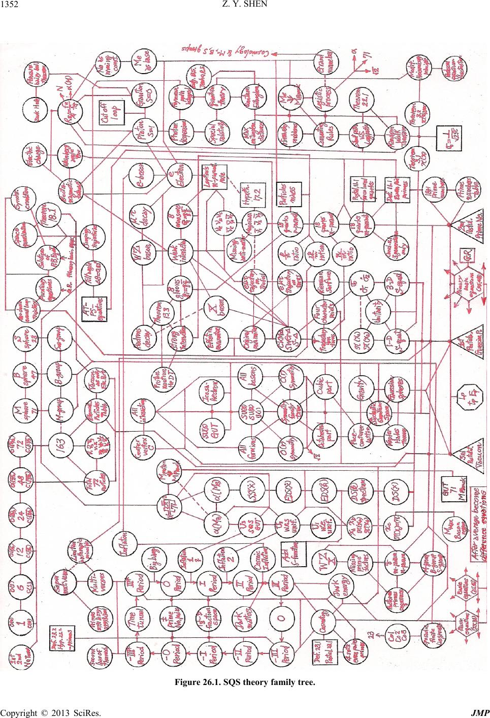

Z. Y. SHEN 1352
Figure 26.1. SQS theory family tree.

Z. Y. SHEN 1353
elements of the Family Tree are shown by 158 circles.
The solid line indicates that, the linked elements are
based on logic deduction, mathematic derivation or fac-
tual correlation. The dashed line indicates that, the linked
elements are somehow correlated.
As shown in the Family Tree, S-equations play impor-
tant roles for SQS theory. The 1-dimensional S-equation,
01)( xS , is the most important one serving as the
foundation. Other S-equations are derived or extended
from this one. Its solutions )( 1
x

, )( 2
x

determine the
location of characteristic points on particles’ model,
which provide physics properties for the particle and its
interactions with others represented by three triangles,
GWS-triangle, CKM-triangle and S-triangle. More works
along this line are needed to complete the task. What is
the function of S-triangle? What does the triangle DBO 11
between CKM-triangle and S-triangle mean? These are
open issues.
The 1-dimensioanal S-equation is a growing point.
Many branches of Family Tree grow from it. The
)(xDS -equation is defined as an extension of the
S-equation and Fourier transformed into )(kDSk
-equation. The)(kDSk-equation on complex k-plane
serves as the spectrum of particles. Fermions and bosons
correspond to local minimums and local maximums of
)( kDSk, respectively. The k-plane spectrum provides
information of mass and a series of possible decay times
for particles. But it leaves two open issues: The mass
value is not uniquely determined; the correlation between
decay times and lifetime is not clearly known.
The )(kDSk-equation is extended by adding two sets of
delta functions to define the )( kEDSk-equation, which
is Fourier transformed back to complex x
-plane as
the )(xEDSx
-equation. Comparing it to the )(xDS - equ-
ation, the additional two summation terms are identified
to represent interactions. In Section 15, these two terms
are used for calculating suppression factors to determine
the characteristic mass values ew
M, ews
M for two uni-
fications based on )( a
x

, )(b
x

and proton mass
proton
M. It was a risk undertaking, because (15.2) is a bor-
rowed formula not from SQS theory first principle and
proton is a composite particle. Fortunately, it worked out
well to provide the mass scales for two unifications.
Moreover, formula (15.15) was found to link ews
M and
GUT
M with )(Z M

. It not only provider legitimacy to the
borrowed formula (15.2) but also reveals the correlation
between proton
M and Planck
M. It eliminates proton
M as a
physics input of SQS theory. In addition, it serves as an
independent confirmation for the interaction terms
in )(xEDSx
-equation.
The )(xDS -equation has a solution at 125.0
1x on
the x-axis corresponding to electron. The
)(xEDSx
-equation no longer has this solution at
125.0
1

x. It is expected, because the adding of two
interaction terms altered its function. To define
)(xSSx
-equation based on )(xEDS x
-equation is an
attempt to restore that function. A solution of
)(xSSx
-equation is found at a new location:
W
i
exx

1
'
,78213151240811255.0'1

x, 1384598708641.28
W

.
The fine structure constant 50359990834.137/1)( 
e
M 
is derived from the value of 1
'x. The importance is the
form of solution shows that, electron is a changed parti-
cle with Weinberg angle W

as a phase angle and the
contribution of electromagnetic energy to its mass by
(9.8) related to )(e
M

. It shows that, the theory is con-
sistent and the extension of )(kEDSk,)(xEDSx
 and
)(xSSx
 from )( kDSk are justified.
The S

-function 1)()(

xSxS did an excellent
job to find the special point730262499871562.0
c
xand
the slightly broken anti-symmetry of )(xS in the re-
gion )5.0,0( from its center 25.0x. It is a very im-
portant finding with many impacts. Point c
x sets the
boundary of the boson states region )5.0,( cdc xxx  .
Fermions’ 1
x and 2
x falling into this region must ap-
pear in pair with anti-particle as a boson state, which is
verified by top quarks’ pair production and e-boson
serving as the inflaton. Point c x also defined two other
special points a
x and b x, which are used to calculate
the values of )( a
x 
, )( b
x 
from the S-equation to de-
termine the mass values for two unifications as mention
previously.
The deviation of 730262499871562.0
c
xfrom
25.0

x is only 5 1028.1~  , but its impacts are huge. It
shows the sensitivity, accuracy and power of the
S

-function and its origin, the S-equation based on SQS
theory first principle.
For the 3-dimensional Gaussian probability, its stan-
dard deviation’s three values show 
120 
symmetry
on the complex plane and set the three branch points on
the Riemann surface to define the two cuts on two layers.
The former provides the first clue for )3(SU group and
the latter leads to the torus model and 4 characteristic
points on its surface.
An important trunk of the Family Tree is rooted from
Gaussian Probability Postulation. The Random Walk
Theorem plays a critical role for many important issues
including converting rules, origin of hierarchy problems,
photon dispersion, the route to GUT etc. In the convert-
ing factor transition region, logistic recurrent process and
random walk process both are in action. The former has a
variable binary probability, while the latter has 6 prob-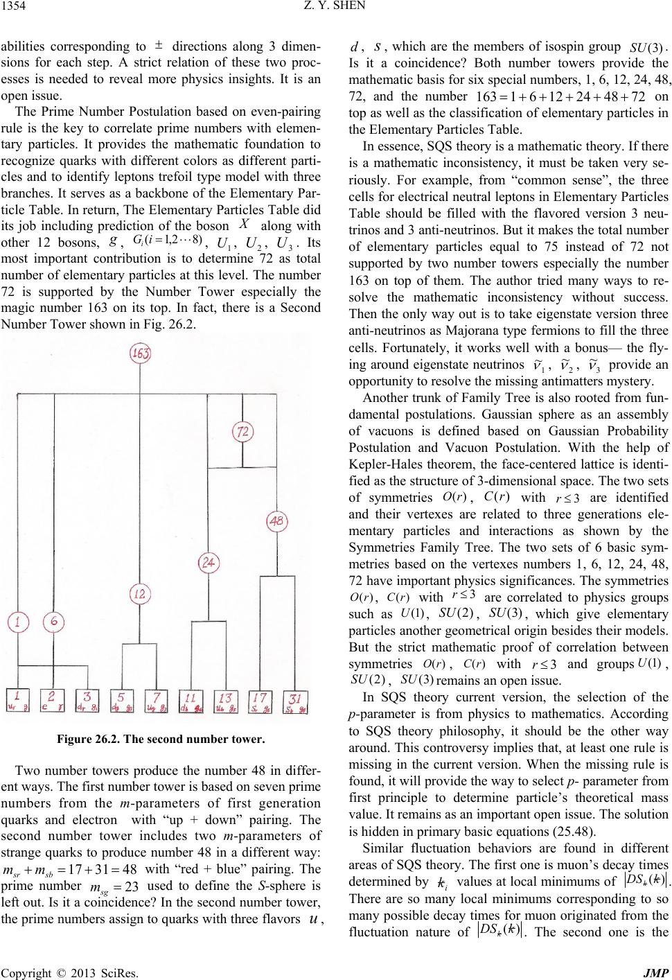

Z. Y. SHEN 1354
abilities corresponding to  directions along 3 dimen-
sions for each step. A strict relation of these two proc-
esses is needed to reveal more physics insights. It is an
open issue.
The Prime Number Postulation based on even-pairing
rule is the key to correlate prime numbers with elemen-
tary particles. It provides the mathematic foundation to
recognize quarks with different colors as different parti-
cles and to identify leptons trefoil type model with three
branches. It serves as a backbone of the Elementary Par-
ticle Table. In return, The Elementary Particles Table did
its job including prediction of the boson
X
along with
other 12 bosons,
g
, )82,1( iGi, 1
U, 2
U, 3
U. Its
most important contribution is to determine 72 as total
number of elementary particles at this level. The number
72 is supported by the Number Tower especially the
magic number 163 on its top. In fact, there is a Second
Number Tower shown in Fig. 26.2.
Figure 26.2. The second number tower.
Two number towers produce the number 48 in differ-
ent ways. The first number tower is based on seven prime
numbers from the m-parameters of first generation
quarks and electron with “up + down” pairing. The
second number tower includes two m-parameters of
strange quarks to produce number 48 in a different way:
483117 sbsr mm with “red + blue” pairing. The
prime number 23
sg
m used to define the S-sphere is
left out. Is it a coincidence? In the second number tower,
the prime numbers assign to quarks with three flavors u,
d, s, which are the members of isospin group )3(SU .
Is it a coincidence? Both number towers provide the
mathematic basis for six special numbers, 1, 6, 12, 24, 48,
72, and the number 7248241261163



on
top as well as the classification of elementary particles in
the Elementary Particles Table.
In essence, SQS theory is a mathematic theory. If there
is a mathematic inconsistency, it must be taken very se-
riously. For example, from “common sense”, the three
cells for electrical neutral leptons in Elementary Particles
Table should be filled with the flavored version 3 neu-
trinos and 3 anti-neutrinos. But it makes the total number
of elementary particles equal to 75 instead of 72 not
supported by two number towers especially the number
163 on top of them. The author tried many ways to re-
solve the mathematic inconsistency without success.
Then the only way out is to take eigenstate version three
anti-neutrinos as Majorana type fermions to fill the three
cells. Fortunately, it works well with a bonus— the fly-
ing around eigenstate neutrinos 1
~

, 2
~

, 3
~

provide an
opportunity to resolve the missing antimatters mystery.
Another trunk of Family Tree is also rooted from fun-
damental postulations. Gaussian sphere as an assembly
of vacuons is defined based on Gaussian Probability
Postulation and Vacuon Postulation. With the help of
Kepler-Hales theorem, the face-centered lattice is identi-
fied as the structure of 3-dimensional space. The two sets
of symmetries )(rO , )(rC with 3r are identified
and their vertexes are related to three generations ele-
mentary particles and interactions as shown by the
Symmetries Family Tree. The two sets of 6 basic sym-
metries based on the vertexes numbers 1, 6, 12, 24, 48,
72 have important physics significances. The symmetries
)(rO , )( rC with 3

r are correlated to physics groups
such as )1(U, )2(SU , )3(SU , which give elementary
particles another geometrical origin besides their models.
But the strict mathematic proof of correlation between
symmetries )(rO , )(rC with 3r and groups)1(U,
)2(SU , )3(SU remains an open issue.
In SQS theory current version, the selection of the
p-parameter is from physics to mathematics. According
to SQS theory philosophy, it should be the other way
around. This controversy implies that, at least one rule is
missing in the current version. When the missing rule is
found, it will provide the way to select p- parameter from
first principle to determine particle’s theoretical mass
value. It remains as an important open issue. The solution
is hidden in primary basic equations (25.48).
Similar fluctuation behaviors are found in different
areas of SQS theory. The first one is muon’s decay times
determined by i
k values at local minimums of )(kDSk.
There are so many local minimums corresponding to so
many possible decay times for muon originated from the
fluctuation nature of )(kDSk. The second one is the

Z. Y. SHEN 1355
fluctuation nature of the complex x
-plane, on which the
value of )( e
M

is calculated from electron’s mass and
Weinberg angle. The value of 50359990834.137/1)( 
e
M

listed in Table 9.1 is from one root of 0)( xSS. In fact,
there is a serious of roots corresponding to different

values, which indicates

as a running constant. The
third one is the fluctuation nature of the PS-equation.
There is a serious of roots or minimums corresponding to
slightly different tilting angles of loop-2 with slightly
different effective parameters’ values. The three types of
fluctuations have something in common. They all are
random in nature, all vary in small steps, and all corre-
spond to real physics parameters. These facts imply that,
they have the same mechanism and come from the same
origin. The mechanism is particles’ discrete trajectories
proved by Theorem 18.1 and related lemmas. A particle
and its parameters are represented by its trajectory on
model surfaces. Jumping trajectories in discrete manner
causes parameters changing responsible to these fluctua-
tion behaviors. Ultimately it is originated from Gaussian
Probability Postulation and stochastic nature of the
quantum space.
In Section 23, the finding of three more sets of prime
number even pairs in prime numbers table is very impor-
tant. Formulas (23.9), (23.10), (23.11) and Conclusion
23.1 indicate that, they are based on the original set of
18+1 prime numbers. With the help of Postulation 23.1,
cosmic history and periods are correlated to elementary
particles and traced back to prime numbers table. It pro-
vides a mathematical explanation for cosmic evolution
from the big bang through inflation(s) up to the current
period. It also predicts the future of universe. Finally it
reaches a conclusion: A cyclic universe oscillates with
alternate expanding and contracting periods. All of these
are built in prime numbers table based on even-pairing
rule. It shows mathematics at work.
As mentioned at the end of Section 23, the universe
during its contracting period, entropy decrease seems
contradictory to the second law of thermodynamics. The
second law is such a fundamental physics law; any viola-
tion is going to shake the foundation of physics. It must
be dealt with. The precondition for applying second law
is that, the statistic ensemble for second law to apply
must be an isolated one. Then the questions become: Is
the universe an isolated statistic ensemble? Is there any-
thing on top of the universe? There are clues from grand
numbers, as listed in Table 24.3, 22
310864.5 F as a
2G grand number is for universe current third period,
44
10686.1 
pre
F as a 4G grand number is for
pre-big-bang period. For reference, the universe contain-
ing 11
10~ galaxies with 22 10~ stars correspond to
1G and 2G grand numbers, respectively.
Hypothesis 26.1: There is a multiverse including
22
10~ universes organized in two levels, each level has
11
10~ members. Our universe is one member of the
lower level sub-multiverse.
SQS theory is not the first one to propose the mul-
tiverse concept. Other theory such as superstring theory
did years ago. Despite the same name, there are differ-
ences. The motivation of SQS theory to propose its mul-
tiverse concept is trying to find a way to resolve the sec-
ond law problem during cosmic contracting period. The
clues are from two grand numbers. The 11
10~ universes
in a sub-multiverse or the 22
10~ universes in the mul-
tiverse correctively form a statistic ensemble for the sec-
ond law to apply. Our universe is just an element akin to
a molecule in the air. The entropy is counted for entire
ensemble not for one element. Moreover, each universe
in the sub-multiverse started from Gaussian spheres
evaporated from pre-big-bang over heated liquid state at
different times in a random fashion. From SQS perspec-
tive, the overall scenario is like that, at a given time, dif-
ferent universes are in their different periods. Some are
expanding and others are contracting akin to six cylin-
ders in a combustion engine. It provides a possible solu-
tion for the second law problem. But it raises a question:
What is the physics links among member universes in the
sub-multiverse serving as the statistic ensemble? It may
have something to do with neutrinos and photons.
Table 26.1 shows mass, Compton wavelength, con-
verting factor, long-path Compton wavelength and maxi-
mum entanglement distance for three types of neutrinos.
Mass values are sited from (17.4), converting factor and
long-path values are calculated according to rules intro-
duced in Section 4. Wavelength

for photon as boson
is replaced by Compton wavelength C


for neutrinos
as fermions. Maximum entanglement distance is changed
accordingly to PCCLd/)4/12(
ˆ
)4/12(2
max  
 for neutrinos.
Table 26.1. Three type neutrinos related parameters*.
*

M,

N are mass and converting factor; C


, C


ˆ are short path and
long path Compton wavelengths.
According to (17.23), the mass of 1
~

and 2
~

are
close to the mass of e

and 

, respectively, the mass
of 3
~

is close to one third of 

mass. For 1
~

with
mass close to e

, the 16
max 10228.1~ d light years
maximum entanglement distance for a pair of entangled
1
~

is 5
10~ times longer than the 10 104.8~ light
years visible universe size. It is capable to reach neigh-
boring member universe territory in the sub-multiverse.

Z. Y. SHEN 1356
For 2
~

with mass close to


, the 11
max 10872.2~d
light years maximum entanglement distance is marginal
to reach neighboring members of the sub-multiverse. For
3
~

with one third of


mass, the
992
max 10139.9)10015.1(3~ d
light years maximum entanglement distance is less than
visible universe size. It is not capable to reach neighbor-
ing members of sub-multiverse. If this is the case, a pair
of entangled 1
~

is eligible to serve as the physics link
between adjacent members of the sub-multiverse. There
is an interesting twist: cross universes connected 1
~

might only oscillate with 2
~

, which is a distinctive fea-
ture different from its non-cross-universes counterpart. It
provides a chance to verify the possible link between our
universe and neighboring universes.
Accordingly, a pair of entangled photons with wave-
length longer than millimeter is also capable to do the job.
The long wavelengths portion of the cosmic microwave
background radiation (MBR) spectrum is in this range. It
may leave some traces there.
In ordinary flat space, max
d sets a limit of the dis-
tance between two entangled particles. But under ex-
traordinary circumstance, things turn out differently. The
edge of visible universe is like the event horizon of a
black hole. The long path link between two entangled
particles is capable to pass through event horizon. It is
possible, because event horizon is defined based on
speed does not exceed the speed of light, the superlu-
minal speed along long path link does not subject to this
restriction.
In Section 25, cosmic MBR photons long-path wave-
length P
L/
2
00
 

at frequency spectrum center wave-
length m
3
01008.1 
 
is used to deal with the dark
energy hierarchy problem. For a double check, let’s use
eigenstate neutrino 2
~

with long path wavelength
m
27
~
2
~10208.1
ˆˆ 


listed in Table 26.1 for an
independent estimation:
123
2
2
~10582.5
ˆ








P
L


. (26.1)
Since anti-neutrino 2
~

is electrically neutral, so the
additional factor 2
4/ 
is not applicable. Comparing
theoretical result 123
10582.5  of (26.1) with observed
data 123
10271.3 

R of (25.35), the relative discrepancy
is 70.6%. The agreement from two independent sources
provides additional support for using converting rule to
deal with dark energy problem. Question: Why use long
path wavelength of 2
~

not 1
~

in (26.1)? Answer: For
an oscillating pair, the one with shorter wavelength sets
the limit. The result of (26.1) is important in another
sense. It confirms that, the factor 2 4/  is applicable
only for the case with electromagnetic force and gravity
involved.
As universe keeps expanding in an accelerating rate,
sooner or later, the distance between universe and its
closest neighboring universe becomes too long exceeding
the maximum entanglement distance of these particles
made the cross universes physics link. Then the second
law ensemble is in trouble. But look at it the other way, it
might provide the cause to trigger cosmic contraction. It
is a wild idea. But it doesn’t hurt to give a thought.
There is another possible scheme to resolve the second
law problem based on the definition of isolated statistic
ensemble. During cosmic contracting period, the uni-
verse boundary is shrinking. Does an ensemble with
shrinking boundary qualified to be an isolated one for the
second law to apply? It deserves a thought. But in any
case, the second thermodynamic law always holds.
In case the second law does not need entanglements to
hold during cosmic contracting period, the multiverse
concept still has a support from grand numbers:
22
310864.5F and 44
10686.1 
pre
F. It indicates that, there
is something 22
10~ times bigger on top of our universe.
Except the multiverse, what else can be?
SQS theory provides a way to resolve the black hole
information paradox. As Hawking suggested, a pair of
virtual photons pops out from vacuum with one outside
and the other inside event horizon. The outside one be-
comes a real photon carrying out part of black hole’s
energy/mass known as the Hawking radiation. Eventually,
the black hole loses its entire energy/mass and vanishes.
The paradox is that, after the black hole vanished, infor-
mation in the back hole is lost. It contradicts to the con-
servation of information according to quantum theory.
From SQS theory standpoint, the two photons entangled
as coherent states interact to each other with superlu-
minal speed along long path link. Like the cosmic entan-
glement case, long path link is capable to pass through
event horizon and transmitting information along with
energy/mass out of black hole via Hawking radiation. In
this way, black hole does not lose any information. In-
formation paradox is resolved. The key is the long path
with superluminal speed.
SQS theory supports its own version of the limited
anthropic principle. Compare to the strong anthropic
principle, it has an important difference. The strong an-
thropic principle is based on the assumption: Physics
laws and constants are different in different universes.
According to SQS theory, there are two different types of
physics laws and constants. The first type based on ma-
thematics such as prime numbers does not change; while
the second type based on geometry may change as the
geometry changes. Any universe as a member of the
multiverse in its third period is governed by 18 prime
numbers serving as the m-parameters of 18 quarks and in
some extent the n-parameters as well. These parameters
cannot change, because they are based on the same sets

Z. Y. SHEN 1357
of 18 prime numbers. SQS theory standpoint is that, for
any universe as a member of the multiverse in its third
cosmic period corresponding to our current universe, the
physics laws and constants may change, but they subject
to strict limitations imposed by a set of unchangeable 18
prime numbers. Our universe nurtured human being on
earth, some other universe in the multiverse with
22
10~  members should be capable to do the same. Su-
perficially this argument seems to restrict the power of
anthropic principle; actually it is to enhance the power of
anthropic principle. If everything including all physics
laws and constants can change arbitrarily, the 22 10~ 
member universes in multiverse are not sufficient to in-
clude even one universe having the set of physics laws
and constants for human being to exist. Then the an-
thropic principle loses its power entirely. Mother Na-
ture may change her mind but not arbitrarily. No one,
not even God, can change the prime numbers.
Back to the multiverse issue,

2
12/71)(
 
M is
defined by (24.33), its values depend on a prime number
71 and a running constant

. For any universe in its
third period, 71 as a special prime number in the
M-group does not change, while

depending on ge-
ometry of particles model may change making )(M

as
a running constant. It supports the SQS theory limited
anthropic principle.
Prime number 71 defined the M-sphere for the current
universe corresponding to a set of 9 even pairs of prime
numbers listed in the first row of Table 23.1. The
pre-big-bang period corresponds to another set of 9 even
pairs of prime numbers listed in the third and fourth rows
of Table 23.1. The prime number located at similar loca-
tion as 71 is 353. Let’s look at (24.33a) for the
pre-big-bang period universe, if 71 is replaced by 353
and kept

unchanged, the value of )(
1M 

is in-
creased about 2552 times. Sine fine structure con-
stant

is related to electrical charge, such big change
is very unlikely. The alternative is:

in denominator
increases approximately 5 times to


5)25.0(

for
compensation. Since the 1-dimensional )(x

carries
information from 3-dimensional space,





5)25.0(
means that pre-big-bang space has much larger area of
negatively curvature corresponding to tremendous repul-
sive force pushing everything outwards. It is a white hole.
As mentioned in Section 23, after-big-crunch universe
transfers into pre-big-bang universe via a time tunnel.
The outlet of time tunnel is a white hole. Here is the
white hole! The two comedies are matched so well. It
was conducted by Mother Nature using mathematic lan-
guage, the actress and actors were prime numbers. If this
argument holds, it serves as another evidence for the
roles played by 71 and 353 in specific and for the corre-
lation between prime numbers and cosmic history in
general.
In fact, 71 is a special prime number in many senses. It
is the largest prime number factor in the M-group factors
sequence. It is in the non-even prime numbers pair
67&71 to end the three generations. It is the radius to
define M-sphere and M-circle. It is the prime number in
formula (24.33a) to define the running fine structure
constant. Noticed that, the sum of three m-parameters for
three strange quarks is:
71312317 



sbsgsr mmm . (26.2a)
Prime number 71 is also related to the Euclid number
7

n for )1!(

n:
1)7654321(1!750417171 





. (26.2b)
This was a mathematic formula introduced by Greeks
two thousand some years ago. Finally, 72171

 is the
total number of particles listed in Elementary Particles
Table. All of these are based on mathematics; no wander
71 played an important role in physics.
Some mathematicians do not recognize 1 as a prime
number. Their definition of prime number is like that: A
prime number is a natural number that has exactly two
distinct natural number divisors: 1 and itself.
For SQS theory, this definition is unacceptable. The
first natural number 1 must be a prime number. There are
mathematical reasons. (1) If 1 is not recognized as a
prime number, the first even pair 3&1 does not exist.
As a result, the first number tower no longer holds. (2)
The second number tower no longer holds either. (3) The
magic number 163 loses its foundation. (4) The symme-
tries family trees lose their foundation. (5) Definition
23.1 and Postulation 23.1 no longer hold. Cosmic history
and future based on it lose their foundation. There are
physics reasons. (1) If 1 is not recognized as a prime
number, up quark r u and down quark r
d do not exist.
The total number of quarks would be 16 instead of 18. A
flavor triplet is in trouble and two color triplets no long
exist. (2) Graviton as rruug

does not exist. (3)
Electron trefoil type model loses its red branch, because
the only even prime number 2/)31(2
er
m corre-
sponding to electron red branch lost its foundation. (4)
Photon as 
ee 
is “handicapped” due to the
“wound” of 
eand 
e. (5) For the current cosmic pe-
riod we live in, the space is 3
2
2-dimensional! What kind
of world is that?
SQS theory is obligated to provide a prime number de-
finition.
Definition 26.1, The Prime Number Definition: A
prime number is a natural number that only has 1 and
itself as its natural number divisor or divisors.
Explanation: Definition 26.1 recognizes 1 as a prime
number. For 1 as a prime number, two divisors happen to

Z. Y. SHEN 1358
be the same. This kind of degenerations is common in
mathematics as well as in physics.
Quantum theory is known for its uncertainty nature
such as Heisenberg uncertainty principle. But the basic
equation of quantum theory such as Schrodinger equation
is deterministic. The uncertainty comes later from the
statistic interpretation of its solution, the square of wave
function’s magnitude *


, serving as probability. SQS
theory introduced uncertainty in the first place with the
Gaussian Probability Postulation. Quantization comes
later. After vacuon introduced in Section 18, Theorem
18.1 and Lemmas 18.1, 18.2 are proved to confirm tra-
jectories’ discrete nature. It serves as the basic quantiza-
tion for SQS theory. In essence, quantum theory is from
quantization to probability, while SQS theory is from
probability to quantization. These two approaches are
quite different.
According to SQS theory, particle’s spin is the angular
momentum of its loop-1 internal cyclic movement. It is
based by the fact that conservation of angular momen-
tums is the sum of spin and trajectory angular momen-
tums combined. Apples can’t add to oranges. Two add-
able terms must belong to the same type. The formula to
calculate a particle’s spin is:
2/
444
11 m
h
m
h
L
L h L
s
PP























. (26.3)
In which, P
mL


1 is the loop-1 circumferential
length, PP L

is the Planck wavelength, mis the
reduced m-para- meter.
For bosons without mass, photon and gluons with
2m have spin s; graviton and massons with
0m have spin 0s. For charged leptons’ trefoil
model three branches together with reduced m-parameter,
1)3/1(3 m, 2/)6/(3 

s. Formula (26.3) is
valid for these particles.
For quarks, all 18 quarks have reduced m-parameter
1m, formula (26.3) is also valid. But it raises a ques-
tion: Is reduction really applicable to quarks? Reduction
means m-, n-, p-parameters reduced with some rate for a
quark, which changes the values of quark’s m-parameter
and n-parameter. As shown in Section 13, strong interac-
tions are based on quarks’ original m-parameter and
n-parameter versus gluons’ m-parameter and n-parameter.
After quarks’ m- and n-parameters reductions, how does
gluon “recognize” quark’s original parameters? In addi-
tion, reduction makes quark’s n-parameter fractional. As
shown in Section 14, leptons’ n-parameters are fractional.
Does the reduction for quarks blur the distinction be-
tween quarks and leptons and the distinction between
strong and weak interactions? These are open issues. In
fact, experiments have found that, some quarks such as
u and d have spin problems. In the meantime, rather
leaves quarks’ spin problem open.
SQS theory does not use operators. It is not the first
one to do so. Feynman’s path integral theory did it dec-
ades ago. Feynman’s path integral equation is equivalent
to Schrodinger’s equation, which shows that quantum
theory can serve its functions without operators. It gives
confidence to SQS theory to go its own way without op-
erators.
In Section 5, SQS theory provided the dispersion equ-
ation (5.7) as a modification for special relativity based
on Planck length P
L. Later in Section 24, the M-sphere
with radius P
Lr 71

is introduced, which serves as a
domain with linear scale longer than Planck length. Ac-
cording to grand number phenomena, large domains with
linear scale of P
NL 11
10~ are possible as shown by
(22.12). The multi-layer domain possibility raises a ques-
tion: Should dispersion equation (5.7) change accord-
ingly? The answer is: Yes. At least the M-sphere is le-
gitimate evidenced by the fact that grand unification oc-
curred on its surface. The dispersion equation (5.7) are
generalized as:

2
/1)(cfLcfv domain  , (26.4a)

2
/1)( 
domain
Lcv  . (26.4b)
domain
L is the length scale of the effective domain. Com-
pare to (5.7), equation (26.4) makes dispersion stronger
and relatively easier for experimental or observational
verification. The results will provide information for ef-
fective domain size. It is important to point out that, if an
effective domain with Pdomain LL  is found, it does not
mean equation (5.7) is abolished and replaced by equa-
tion (26.4). Photon dispersion equation (5.7) is funda-
mental based on space basic grainy structure, which is
always valid no matter higher level domain exists or not.
This is the reason that equation (26.4) is defined as a
generalization not a replacement of original dispersion
equation (5.7).
Quantum mechanics is a very successful theory in
terms of extremely high accuracy and very broad practi-
cal applications. But it has many contradict versions of
interpretation and seemingly none of them is commonly
accepted. SQS theory provides an opportunity for a new
interpretation. The key is the meaning of locality. As
discussed in Section 5, if locality means interactions and
information transmission are restricted by speed of
cv

under any circumstances, the superluminal phe-
nomena found by many experiments between entangled
particles inevitably lead to “spooky action at a distance”.
The long path provides a way out. Entangled particles are
linked by long path. It is a physical entity for interactions
and information transmission along it with superluminal
speed cNcv 

ˆ seen by stationary observers. In
this way, locality is reserved and many other “spooky
actions” in quantum mechanics can be interpreted with
common sense. This is a topic with very important phys-

Z. Y. SHEN 1359
ics and philosophical significances for further investiga-
tions. SQS theory standpoint is clear: Einstein was
right — “No spooky action at a distance.”
General relativity is a beautiful theory. Based on two
principles, general relativity provides a set of Einstein
equations for gravity in terms of space-time curvature. It
has been verified by many experiments and observations
without even one failure. General relativity serves as one
of two pillars for modern physics. The problem is that,
general relativity is not compatible with quantum theory.
For decades, there were many attempts to quantize gen-
eral relativity and none of them is commonly accepted.
From SQS theory viewpoint, it is the time to rethink the
issue. In fact, this is the initial inspiration for the author
to search SQS theory basic equations.
As mentioned in Section 25, the key concept for SQS
basic equations based on Einstein original equations
(25.1b) is to introduce uncertainty to gauge tensors by
Postulation 25.1. From SQS theory perspective, the con-
cept is very clear to begin with: To unify general rela-
tivity with quantum theory, uncertainty is primary
and quantization is secondary. The other key concept is
to introduce the intrinsic time by (25.5), which naturally
leads to the superluminal speed for vacuons movements
inside elementary particles and the appropriately adjust-
ment of separation for the variable in difference equa-
tions of (25.31) and (25.43) etc. Both concepts paid off
tremendously as shown in Section 25.
Standard Model (SM) is proved to be a successful ef-
fective theory with enormous theoretical results agreed
very well with experimental data. As shown in previous
sections, many results from SQS theory are agreed well
with experimental data. There must be a strict link be-
tween SM and SQS theory. When the link is found, some
open issues will settle down.
On the other hand, there are some differences between
SM and SQS theory.
The first one is the difference ways to treat particles.
SQS theory provides trajectories on models to represent
elementary particles, while SM treats them as points.
This is the reason that, SQS theory does not have diver-
gence problem and does not need renormalization. There
are deeper reasons for SQS theory to avoid divergence
problem. For the long range force such as electrostatic
force, its strength is inversely proportional to the square
of distance. As distance approaches to zero, its strength
and energy density approach to infinity causing diver-
gence. According to SQS theory, electromagnetic force is
unified into gravity at length scale PGUT LL 71 on
M-sphere surface. So there are no infinity and no diver-
gence for electromagnetic force. For gravity, its strength
is also inversely proportional to the square of distance. It
keeps that way until P
Ll 3~ as shown in Fig.25.1. At
PPcLLxl 3026452998715627.0 , gravitational force
vanishes. In the region PcLxl 0, it becomes repul-
sive. So there is no divergence for gravitational force. In
fact, this is the way SQS theory eliminated singularity.
Within the M-sphere, two short range forces are unified
into gravity, so there is no divergence either.
The second one is the different ways to introduce pa-
rameters. SM has twenty some handpicked parameters
from experimental data, while SQS theory has three sets
of mathematical parameters. In which two sets mostly are
determined prime numbers and the other set is deter-
mined by particle’s mass in the current version. In es-
sence, the second difference is originated from the first
one. It is understandable that, one can derive parameters
from a geometric model with trajectory and characteristic
points, but no one can derive any parameter except its
location and movement from a point.
The third one is SM does not include gravity, SQS
theory does. In fact, SQS theory unified all interactions
to gravitational interaction as shown in Section 15.
The fourth one is the number of elementary particles.
As shown in Table 18.1 and Table 18.2, SM has 25 par-
ticles not including anti-particles, while SQS theory has
72 particles. The difference is stemmed from SQS theory
recognized quarks with different colors as different parti-
cles. After the vacuon introduced, the difference becomes
the other way around with only one ultimate elementary
particle for SQS theory.
SM is a well-developed theory. With decades of coop-
erative efforts, it is capable to calculate the cross sections
and branching ratios for particles and interactions from
Feynman diagrams, which are agreed with experiments
very well. SQS theory is a developing theory. It just gets
started. It hasn’t done these type calculations yet but has
the potential to do so. The potential is based on proper-
ties of SQS theory. One is in the 1-dimensional
S-equation, in general the probability at 1
x has excess
and the probability at 2
x has deficit. For most particles,
the excess does not match the deficit exactly. The mis-
match provides the mechanism for the particle to interact
with others or transfer to others. The other one is jump-
ing trajectories, which also provide the opportunity for
the particle interacting with others or transferring into
others. These two properties are intrinsically correlated
based on primary basic equations (25.48). For instance,
as shown in Section 25, different elementary particle
represented by different vertexes in


2/1O share the
same center vertex. It serves as a junction of their overall
closed geodesic loops, which provides the mechanism for
interactions among particles. So SQS theory does have
the potential to provide the method for calculating cross
sections and branching ratios. This is an important open
issue. It wouldn’t be easy and may require some tricks
and extensive number crunching. But in principle it is

Z. Y. SHEN 1360
feasible. Hopefully, it can be done in the near future.
SQS theory does not intend to compete with SM. It
provides geometrical models and mathematical interpre-
tations to support SM at a deeper level. It also provides a
way to make SM as a quantum theory compatible with
general relativity.
There are similarity between super-symmetry theory
and SQS theory. Both theories require fermions and bo-
sons somehow matching to each other. But there is an
important difference. All hypothetic particles predicted
by super-symmetry theory such as the “s- ” for bosons
and the “-o” for fermions are not discovered yet. In SQS
theory Elementary Particles Table, there are no undis-
covered fermions; for the 24 bosons, 13 of them are
waiting to be discovered. If the 8 massons are indeed
attached to W, Z, X bosons, the number of undiscovered
bosons is reduced to 5. The difference between su-
per-symmetry theory and SQS theory is stemmed from
the different ways to match fermions and bosons. Su-
per-symmetry theory does not look for possible matches
in existing elementary particles, while SQS theory does.
In fact, all fermions and bosons in Table 18.2 are
matched, in which only 13 bosons are hypothetical.
There are some similarities between SQS theory and
string theory [21]. After all, strings and trajectories both
are 1-dimensional objects representing elementary parti-
cles. In this regard, these two theories do have some
common grounds. In addition, for SQS theory the way to
introduce mass by adding oscillating mass terms in the
AT- equations and PS-equations is inspired by string the-
ory. But there are major differences.
The first difference is the number of space dimensions.
Superstring theory is based on 9-dimensional or
10-dimentional space (the early version of string theory
was based on 25-dimensional space), while SQS theory
is based on 3-dimentional space. As shown in Sections
22, the physics groups are related to two set of symme-
tries, )(rO and )( rC with 3

r, which are the intrin-
sic property of the 3-dimensional space with
face-centered lattice structure. It includes two parts, the
cubic part and the octahedral part. The face-centered lat-
tice structure can be viewed as an octahedron imbedded
in a cube. Someone may interpret the imbedded octahe-
dral part as the hidden space. For instance, )2/1(O
symmetry centered at 1 octahedral vertex has 12 vertexes
on the spherical surface. The 6212  pairs of ver-
texes related to the center vertex form 6 non-orthogonal
axes, which might be interpreted as a 6-dimensional
space hidden in a 3-dimensional space represented by the
cubic part. From SQS theory perspective, it is an illusion
of the face-centered space structure. The argument is to
state SQS theory viewpoint and by no means to criticize
string theory. After all, what is the number of space di-
mensions? 9? 10? 25? or 3? Only experiments can an-
swer.
The second difference is the nature of string and tra-
jectory. String theory treats string as a vibrating thread
with mass and elasticity. SQS theory treats trajectory as a
path of vacuons movement. This difference makes the
other difference. For some version of the string theories,
except graviton, all other elementary particles are repre-
sented by open strings; only graviton is represented by
closed string. For SQS theory, except graviton, all other
elementary particles’ trajectories are closed loops. The
reason is that, in general, vacuons movement along tra-
jectory cannot stop suddenly and revise directions ab-
ruptly. As the only exception, graviton stops at cubic
vertex i
x and changes its directions. It has specific rea-
sons based on Theorem 3.2, Theorem 4.1 and Theorem
22.1.
The third difference is the topological structures of
elementary particles. The particle models proposed by
SQS theory are topological manifolds with genus num-
bers of zero, one, two and three. String theory has so
many different Calabi-Yao manifolds with possible
numbers up to500 10 . If the model does represent an ele-
mentary particle, it should provide particle’s all physics
parameters from its geometrical parameters. SQS theory
did so with models having genus number not exceeding
three. The key is model having definitive shape and size
plus characteristic points and related triangles. Model’s
shape and size are determined by particle’s m-, n-,
p-parameters; its characteristic points’ location and re-
lated triangles are determined by )( 1
x

and )( 2
x

as
messengers carrying information from the S-equation. In
principle, the particle’s all physics parameters can be
derived from these geometry parameters. On the other
hand, if the topological manifold has no definitive shape,
size and lack of characteristic points, the only way for it
to represent an elementary particle with all physics pa-
rameters is to increase its genus number. Again, it is by
no means to criticize string theory. What type of strings
or trajectories and models elementary particles really
have, only experiments can tell.
The fourth difference is fermions versus bosons. The
original string theory based on 26-dimensional space-
time had only bosons. Fermions were introduced later via
super-symmetry to form the superstring theory. For SQS
theory, fermions are primary, bosons made of a pair of
fermion and anti-fermion are secondary. Boson or fer-
mion, which one is primary? This is the question. A basic
theory should answer.
Over the years, string theory has accumulated so many
mathematic achievements and some physics insights. It
takes time for SQS theory to learn. Hopefully, more mu-
tual understandings will benefit both theories.
There are similarities between SQS theory and the

Z. Y. SHEN 1361
loop theory [22]. One similarity is obvious. Both theories
are basically dealing with loops. There is another impor-
tant similarity. One of the major merits of loop theory is
background independence. Space structure is not a priori
determined; instead, it emerges naturally. SQS theory
supports background independence. In intermediate and
macroscopic scales, the moving around M-spheres ar-
range themselves according to distribution of mass and
energy to satisfy basic equations (25.31) the same way as
general relativity. Inside the M-sphere, Gaussian spheres
arrange themselves in face-centered lattice structure to
reach minimum potential energy. Inside the Planck cube,
the primary basic equations (25.48) provide a mechanism
for background independence based on the stochastic
behavior of geodesics adjusting gauge tensors as shown
in Section 25.
Composite preons theory is based on preons triplets to
form topological models for elementary particles [23,24].
In SQS theory, charged leptons and neutrinos trefoil tra-
jectories have three branches. For quarks, there are flavor
triplets and color triplets. In its current version, compos-
ite preons theory does not provide detail information
regarding elementary particles’ parameters for further
comparison.
Striking similarities between crystallography and par-
ticle physics were found [25]. For SQS theory, it is not
only similarity; the microscopic space is a crystal with
face-centered lattice structure. All elementary particles,
interactions and symmetries are originated from it. This
area deserves further investigation based on the
face-centered lattice structure. Hopefully, they will give
SQS theory more supports and inspirations.
Technicolor theory is proposed as an alternative of
higgs mechanism to provide mass for particles with mass
[26]. There are some similarities between technicolor
theory and SQS theory. The eight hypothetic massons
i
G (82,1i) introduced in Section 14 are pure mass
stuff. Massons contribute a portion of mass for gauge
bosons W, Z and X. If 1
U, 2 U, 3 U are indeed made
neutrino and anti-neutrino pairs, the tremendous mass
gap between the “heaviest” and the “lightest” would be
also filled by vast numbers of massons. From SQS theory
perspective, massons provide a portion of mass to bosons
with mass. Whither massons also play a role to provide a
portion of mass for some fermions, it is an open issue.
According to SQS theory, particles’ mass is determined
by e
MMnp// ratio and generated by sinusoidal oscil-
lation of mass term


)/2(sinmp along trajectory,
which is ultimately originated from solutions of primary
basic equations (25.48). It serves as the universal mecha-
nism of particles’ mass for SQS theory. But it does not
necessarily mean no common grounds for Higgs mecha-
nism, technicolor theory and SQS theory. There are pos-
sible correlations among these theories, which deserve a
close look.
The original Grand Unification Theory (GUT) in-
tended to unify three interactions excluding gravity was
based on )5(SU group [27, 28]. Despite the same name,
it is different from SQS theory GUT including gravity.
The GUT based on )5(SU is an elegant theory. Ac-
cording to the minimal )5(SU model [28], protons are
not stable and decay with lifetime of 7.129
10~ 
years.
Unfortunately, this prediction was disproved by Ir-
vine-Michigan-Brookhaven (I-M-B) experiment and later
by Super-Kamiokande (S-K) experiment. It was such a
disappointment, afterwards physicists moved on other
directions. From SQS theory perspective, there are rea-
sons to believe the original GUT based on )5(SU
group might have a chance for revival.
The protons predicted lifetime of 7.129 10~   years
is based on )5(SU group. The obvious precondition is
that, )5(SU group must be in existence in the first
place. It is well known in crystallography that, 5-fold
symmetry does not exist in single-crystal structure; it
exists in the quasi-crystal structure with quasi-periodic
lattice lengths [29, 30]. The quasi-crystal lattice must
have at least two different spatial periods with irrational
ratio. The face-centered space structure in its sin-
gle-crystal form does not support )5(SU group. For
)5(SU group to exist, the face-centered space structure
must have defect to accommodate 5-fold spatial symme-
try.
As show in Fig. 26.3, icosahedron has 5-fold spatial
symmetry. Like )2/1(O symmetry, icosahedron also
has 12 vertexes on a spherical surface with radius:

































 2
95105652.0
5
2
sin
22
5210
4
1
cos
p
PP
i
L
LL
r

.
(26.5)
The relative deviation of


2/95105652.0
cos pi Lr 
from 2/
)2/1( P OLr  is 4.9%.
The icosahedron has 20 connected equilateral triangles
on its surface. It has sufficient room to accommodate
quarks ),,( bgruuuu ,),,( bgr uuuu ,),,( bgrdddd and
leptons participated in the proton )(uudp decay proc-
ess.
According to Kepler-Hales theory, space based on
Gaussian spheres with face-centered lattice structure is
the ground state of vacuum with lowest potential energy.
An icosahedron as defect in face-centered space structure
is in a quasi-stable state with higher energy. To accom-
modate 5-fold symmetry, the 12 vertexes of )2/1(O
must shift locations converting to icosahedron structure.
The conversion process is governed by probability.
Assume a vertex stays in )2/1(O and shifts to icosa-
hedron with equal probability 2/1 . The probability for
12 vertexes of )2/1(O all shift to icosahedron is


.4096/12/1 12 pFor a tank of water containing

Z. Y. SHEN 1362

3231101010~MN protons with lifetime 31
10~ 
years, one originally expected to detect 10M decay
events per year. This expectation is based on the assump-
tion that, )5(SUgroup is fully applicable to all
N
pro-
tons involved. But it is not true, because for N protons
only
pN
protons are eligible for )5(SU group to apply.
Take this effect into account, for the water tank contain-
ing

3231 101010~ MN protons, the expected num-
ber of proton decay events should be multiplied by
probability p and become
 00244.04096/11010

p
per year. Instead 10 decay events per year, the real ex-
pectation is ~2.4 events per 1000 years. According to this
argument, I-M-B type and S-K type experiments should
increase the number of protons in tank by at least 1000
times.
Figure 26.3. Icosahedron with 12 vertexes and 20 equilat-
eral triangles has 5-fold symmetry.
There are also questions regarding the validity of
I-M-B type and S-K type experiments. As shown in Sec-
tion 7, in the time interval stt 13
min 10075.20
 ,
muons have zero probability to decay. What is proton’s
min
t? If proton’s yearst 11
min 10~, even all protons were
born at big bang 10
1037.1 years ago, none of them is
eligible for decay yet. If this is the case, to increase the
number of protons for I-M-B type and S-K type experi-
ments would not help at all, the only way is to wait until
.
min
tt 
In Section 15, SQS theory borrowed a method from
GUT based on )5(SU group to calculate the character-
istic mass for two unifications. This method is proved to
be equivalent to the one with more credibility. It shows
that, there is some truth in )5(SU group. For instance,
)5(SU group breaks down to )1()2()3( USUSU

,
which are the right ones for elementary particles and in-
teractions in the standard model. Moreover, )5(SU
group contains 24 bosons, in which 13 of them called
“X-bosons” are hypothetic. As shown in the Elementary
Particles Table, SQS theory also has 24 bosons, in which
13 are hypothetical. Is this a coincidence? It is worth-
while to investigate )5(SU group to find out its relations
with )(rO and )(rC symmetries. The bottom line is
that, as long as )2/1(O can convert to icosahedron
with 5-fold symmetry, proton has a chance to decay. The
question is: Under what condition and what’s the prob-
ability? This is an interesting open issue worthwhile to
explore.
Elementary particles’ models proposed by SQS theory
are listed in Table 26.2.
Most models listed in Table 26.2 have been explained
in previous sections. A few models need some explana-
tion. The spindle type torus models are listed as genus-0,
because their center hole(s) are covered. The topological
manifold is allowed to continuously deform, but the
heavy mass Max
MM requires da 
2
' preventing the
center hole to be uncovered. For gauge bosons W, Z, X
and scalar bosons 1
U, 2 U, 3 U with heavy mass
Max
MM , their models belong to two joint spindle type
torus with genus-0.
Table 26.2. Summary of elementary particles models.
In algebraic topology, Henri Poincare discovered the
“hairy ball theorem” [31]. Imagine a ball with a hair
growing out from every point on its surface. One tries to
comb the hairs flat and smoothly around the ball. Put in
mathematic terms. “Hairs” correspond to nonzero tangent
vector field made of a set of tangent vectors. “Comb the
hairs around the ball” is to arrange the tangent vectors
around the closed surface. “Flat” means tangent vectors
pointing only at tangential direction of the closed surface.
“Smoothly” means tangent vectors arranged with conti-
nuity without abruption.
Poincare theorem proved that, no matter how to ar-
range these tangent vectors (hairs), it always leaves some
crown (bundle of hairs) stretched out from the ball sur-
face. Poincare theorem is valid for any genus-0 closed
surface topologically equivalent to the ball surface. Fig.
26.4 shows two crowns on a spherical surface.

Z. Y. SHEN 1363
Figure 26.4. “Combed hairs” on spherical surface as ge-
nus-0 manifold with two “crowns”.
There are two closed surfaces, on which hairs can be
combed flat and smoothly without crown. One is genus-1
torus with one center hole and the other is Klein bottle.
In 3-dimensional space, closed surfaces are classified
into two types: Type-1 surface with genus number equal
to 1 and Type-2 surface with genus number other than 1.
According Poincare theorem and related rules, Type-1
closed surface does not have crown and Type-2 closed
surface has at least two crowns.
From SQS theory perspective, Poincare theorem and
related rules provide important clues for elementary par-
ticles’ models, trajectories and interactions. As shown in
previous sections, particle’s trajectories are on its mod-
el’s closed surface (the small holes on torus surface are
closed by filling points according to Penrose [2]). For a
trajectory on model surface, the tangent vectors along its
path are flat and smooth. For a set of trajectories on the
model surface, the tangent vectors along these trajector-
ies are arranged like combed hairs. According to Poin-
care theorem and related rules, for the set of trajectories
on the model’s Type-2 closed surface, there are always
crowns for trajectories to jumping out or jumping in.
Jumping literarily means vector must leave the surface,
which makes it no longer tangential and abruptly chang-
ing directions. This is what happens at the crowns.
As described previously, jumping trajectories are
equivalent to interactions. Therefore, a particle having
interactions must be capable to jump trajectories and its
model surface must have crowns. The requirement for
crowns is met for Type-2 model with genus number other
than 1. The problem is the fifteen quarks with genus-1
torus model: r
u,g
u,, b
u,, r
d,g
d,b
d,r
s,g
s,b
s,r
c,g
c,
b
c,r b,g
bb
b.. The genus-1 torus belongs to Type-1,
which has no crown. If this is really the case, there would
be no electromagnetic interaction, no strong interaction
and no weak interaction for these fifteen quarks. Obvi-
ously, it is not true. One possible way to solve the prob-
lem is to leave same of four tiny holes open on torus sur-
face, which makes their model as open surface to have
crowns. For instance, leaving two tiny holes open at
characteristic points
A
and
B
creates two crowns. It
serves as a working assumption for SQS theory.
In topological terms, free flying photon with genus-1
model of Type-1 has no crown meaning no interaction
among photons. In fact, electromagnetic interactions are
linear and photons do not interact with each other. It is
also evidenced by the fact that, Maxwell equations are
linear equations. It serves as a supportive evidence for
the effectiveness of Poincare theorem and related rules in
particle physics.
Gluon’s genus-2 model of Type-2 has crowns indicat-
ing that, there is interaction among gluons. In fact, strong
interaction mediated by gluons is nonlinear and gluons
interact with each other as shown in Table 13.5. It also
serves as another supportive evidence for the effective-
ness of Poincare theorem and related rules in particle
physics.
Graviton’s genus-0 model of Type-2 has crowns. They
should interact with themselves. In fact, as the mediator
of gravity, graviton interacts with anything having mass
and energy. The flying around gravitons have energy and
dynamic mass for gravity to act upon. It is also evidenced
by the fact that, Einstein equations of general relativity
are nonlinear equations and nonlinearity represents
self-interaction. The gravity among gravitons is ex-
tremely feeble, but it does exist. It supports graviton with
genus-0.
Conclusion 26.1: Graviton is a scalar boson with
spin 0.
Explanation: Poincare theorem and related rules serve
as the topological evidence for Conclusion 26.1, graviton
must have spin 0. Let’s consider the opposite. If graviton
has spin 2 or any other nonzero spin values, its closed
loop model belongs to genus-1 of Type-1 without crown
corresponding to no interaction among gravitons. It is
obviously not true. This is a conclusive evidence for gra-
viton having spin 0 as stated in Definition 18.1 based on
other mathematic reasons.
Black hole with closed event horizon is a genus-0 ma-
nifold of Type-2. According to Poincare theorem, black
hole must have crowns and hairs. Therefore, Hawking
radiation is not only a possibility but also a necessity. It
serves as a mathematic support for Hawking radiation
and the solution for information paradox suggested by
SQS theory.
Poincare theorem and related rules also support an
“absolute black hole” with no stretched out hair.
Definition 26.2: Absolute Black Hole. A chuck of
matter with total mass exceeding critical mass to form a
manifold with genus-1 torus event horizon is defined as
an absolute black hole.
Explanation: The name “absolute black hole” is cho-
sen to differentiate it from black hole. Black hole has
Hawking radiations as stretched out hairs. Absolute black
hole has no radiation and no stretched out hair.

Z. Y. SHEN 1364
Theorem 26.1: No Radiation Theorem. Absolute
black hole has no radiation of any kind.
Proof: According to Poincare theorem with related
rules and Definition 26.2, absolute black hole with ge-
nus-1 torus event horizon has no crown and no stretched
out hair which means no radiation. QED
Lemma 26.1: Hawking Mechanism. Absolute black
hole has no Hawking radiation, but it has Hawking me-
chanism. A pair of virtual photons pops up in the vicinity
of absolute black hole’s event horizon. One photon falls
into absolute black hole, and the other photon is kept in
the event horizon. This Hawking mechanism process
keeps going on. As results, more and more photons are
circulating in absolute black hole’s event horizon like
“combed hairs”.
Proof: The Hawking mechanism is the same as that
occurred in the vicinity of ordinary black hole. The only
difference is that absolute black hole has no “crown”,
therefore photon cannot radiate. QED
Lemma 26.2: When two absolute black holes collide
in proper ways, they transfer into a regular black hole
with genus-0 event horizon or a special black hole with
genus-2 event horizon. Both subject to Hawking radia-
tion.
Proof: According to Poincare theorem with related
rules and Theorem 26.1, the regular black hole with ge-
nus-0 event horizon or the special black hole with ge-
nus-2 event horizon has crowns and stretched out hairs
— radiation. QED
The boundary of visible universe like black hole’s
event horizon is a genus-0 manifold of Type-2. Accord-
ing to Poincare theorem, it must have crowns. Therefore,
the cross universes connections via entangled 1
~

, 2
~

and cosmic MBR photons not only are possible but also
are necessary. It serves as an independent mathematic
support for the multiverse concept and the physics con-
nections among its member universes.
So far everything is consistent. It indicates that, Poin-
care theorem in particular and topology in general play
critical role for elementary particles’ models, trajectories
and interactions as well as for cosmology. It is mathe-
matics at work.
According to Green et al [21], spinors may relate to
the tangent vectors in Poincare theorem. Spinor is the
basic concept of spinor theory [32]. The relation between
spinor theory and SQS theory is an open area. Spinor
theory is based on complex space, while SQS theory is
based on real space except the abstract 3 complex planes
associated with 3 axes introduced in Scheme-2 of Section
3. What is the implication of real space versus complex
space is an interesting topic.
SQS theory provided a framework for cosmology
based on prime numbers with results agreed to cosmol-
ogy standard model plus some new insights. But some
important issues left open such as: (1) How many cosmic
inflations did happen, one, two or three? (2) What is the
mechanism of 3
1
1-dimensional space in the first period
transferred into 2-dimensional space in the second period?
(3) Based on mathematics, is there a way to reveal cos-
mic history and to predict cosmic future in more details?
(4) When will the current accelerating cosmic expansion
end? (5) Are there more cosmic “secretes” hidden in
prime numbers? In fact, there is one.
It is interesting to find another set of 13 consecutive
even paired prime numbers listed in Table 26.3. It starts
from 2791&2797 and ends at 2999&3001. The two
prime number odd pairs are 2777&2789 and 3011&3019
marked with underline to start and to stop the even paired
prime number sequence at two ends.
Table 26.3. The prime numbers between 2707 and 3083 and 13 consecutive even pairs
2707 2711 2713 2719 2729 2731 27412749 2753 2767 2777 2789
2791 2797 2801 2803 2819 2833 2837 2843 2851 2857 2861 2879
2887 2897 2903 2909 2917 2927 2939 2953 2957 2963 2969 2971
2999 3001 3011 3019 3023 30373041 3049 3061 3067 3079 3083
The set of 13 even prime numbers pair represents

3
1
4dimensional space without temporal dimension. The
product of 26 prime numbers in this set is:
.10642.9300129992971296929632957
2953293929272917290929032897288728792861
2857285128432837283329192803280127972791
89




S
F
(26.6)
In the 13 consecutive even pairs representing

3
1
4di-
mensional space, the one additional even pair served as
fractal mechanism to change dimensions.
Based on S
F, two prime number products are defined
as:
27
410948.328432837283328192803280127972791  S
F,
(26.7a)
.10442.230012999297129692963295729532939
2927291729092903289728872879286128572851/
62
49










SSS FFF
(26.7b)
In which, 4S
F is the product of 4 consecutive even
pairs in the beginning part of S
F and 9S
F is the prod-
uct of the other 9 consecutive even pairs.
As shown in Section 23, the product 22
310864.5 F

Z. Y. SHEN 1365
as a 2G grand number corresponds to the universe in
current period. The product 44
10686.1
pre
F as a
4G grand number corresponds to the multiverse in
pre-big-bang period. It seems natural to assume that, the
product 89
10642.9
S
F as a 8G grand number
corresponds to the precursor of the “super-multiverse”.
Hypothesis 26.2: Super-Multiverse. There is a su-
per-multiverse including 45
10/~
preS FF mul-
ti-universes organized in two levels, each level has
22
10~ member multiverse. Our multiverse is one member
of the lower level. The total number of universes in the
super-multiverse is 67
310~/~ FFS.
Hypothesis 26.2 serves as a foundation to explore pos-
sible physics implications of S
F related issues.
Hypothesis 26.3: Big Start. The super-multiverse
started at the big start, which is the beginning of time.
Before the big start, everything was static without any
variation. Time started at the big start, everything started
to develop.
Before the big-start, the 
4
1
4dimensional space cor-
responding to S
F without temporal dimension wasstatic,
in which everything was at a standstill without any
movement. The mass/energy was “frozen”.
The big start was the beginning of time, temporal di-
mension split from the 4
1
4-dimensional space. The
)13(-dimensional space-time corresponding to 4S
F
was born. The mass/energy carried out by 4S
F became
dynamic and the super-multiverse started to evolve. The
mass/energy corresponding to 49 /SSSFFF served as
the precursor of dark energy and dark matter. The
mass/energy carried out by 4S
F served as the precursor
of ordinary matter/energy, which was the “raw material”
of the ordinary elementary particles and energy to build
the planets, stars and galaxies in the super-multiverse.
The concept of changing space-time dimensions is
checked with two ways. One way is given by9S
F in
(26.7b). The other comparative way is to treat spatial
dimensions as the exponentials ofS
F. As space changed
from 3
1
4-dimensional to 3-dimensional:
 
62
4
3
89
4
3
1098.11042.93
1
3
1
S
F. (26.8)
Comparing to 62
910442.2  S
F, the result of (26.8)
has a relative deviation of 18.9%. For two large numbers
difference with 62 orders of magnitude, the 18.9% rela-
tive deviation serves as a check for the validity of
changing space-time dimensions based on three products
4S
F, 9S
F and 94 FSS FFF .
After the big-start, according to Hypothesis 26.2, the
super-multiverse kept expanding and splitting to form
multi-level multiverses and universes. The mechanism of
space expansion is Planck cubes’ splitting. As the origi-
nal one super Planck cube split into
N
Planck cubes,
the mass/energy in a Planck cube decreases according to
1
N rate, and the mass/energy density decreases accord-
ing to 2
N rate. Correspondingly, the ratio of the super
Planck density at big-start versus the ordinary mass/ en-
ergy density in the current universe is estimated as:

124
2
9
2
4
10965.5 






S
S
SF
F
F
R. (26.9)
Notice that, in the two previous estimations, the theo-
retical values of (25.36), (26.1) and the observed ratio
123
10271.3 
obserbed
Planck
R



of (25.35) all are based on Planck density versus overall
density including the contributions of ordinary matter,
dark matter and dark energy. According to cosmic ob-
servation and cosmic MBR data, the universe contains
4% ordinary matter, 23% dark matter and 73% dark en-
ergy. Taking this factor into account, the value of (26.9)
should be adjusted as:

123
2
9
2
4
10268.3
%73
%4
%73
%4
%73
%4
'


























S
S
SF
F
F
RR .
(26.10)
Compare the value of (26.10) with 123
10271.3

R
of (25.35), the theoretical result 123
10268.3' R has a
relative deviation of 4
1017.9  .
Three theoretical results for the dark energy hierarch
problem are listed in Table 26.4 to compare with ob-
served data.
Table 26.4. Theoretical results for dark energy hierarch
problem compare to observed data.
The comparison says all.
As shown in Section 23, the legitimacy of three cos-
mic periods, Period-I, Period-II and Period-III*, were
verified by (23.9), (23.10), (23.11) and summarized in
Conclusion 23.2. It shows that, the prime number corre-
sponding to these three periods are closely correlated to
the prime number corresponding to current period, Pe-
riod-III. Let’s verify the legitimacy of the big start with
prime number products S
F. The following formulas are
based on the prime numbers corresponding to cosmic
periods listed in Table 23.1 and Table 26.3.
The first prime number in product sequence S
F is
2791, which is closely correlated to the prime numbers

Z. Y. SHEN 1366
corresponding to Period-III, Period-II, Period-

and
Period-III*.




).117()321(
263257251241239
197193191181179
113109107103101
1311753212791
*










IIIPeriod
IPeriod
IIPeriod
IIIPeriod
(26.11)
The rules in (26.11) are similar to the rules in (23.9).
As shown on right of (26.11), prime number 2791 is the
sum of 4 sets of beginning prime numbers in parenthesis
for Period-III, Period-II, Period- and Period-III* plus
(1 + 2 + 3) and (7 + 11). The repeat of three prime num-
bers (1 + 2 + 3) represents the fact that, the space corre-
sponding to product sequence S
F is 3
1
4-dimen-
sional. The repeat of two prime numbers (7+11) repre-
sents the fact that, there is a temporal dimension hidden
in the product sequence 4S
F. For the Period-
, the two
prime numbers 167 and 173 at beginning of the sequence
are omitted to transfer Period- with )1( 3
1
- dimen-
sion space into Period-  with 1-dimension space to
avoid redundancy. Otherwise, the sum of Period-I and
Period-II would be )3( 3
1
-dimension space contradic-
tory to Period-III with 3-dimensional space.
The last prime number in product sequence S
F is
3001, which is closely correlated to the prime numbers
corresponding to Period-III, Period-II, Period-

and
Period-III*.




).321()5()19()43(
317331337347
191193197199
139149151157
475359613001
*











IIIPeriod
IPeriod
IIPeriod
IIIPeriod
(26.12)
The rules in (26.12) are similar to the rules in (23.10).
The order of summation in (26.12) is backwards from the
last prime numbers 61, 157, 199, 347 of prime numbers
sets corresponding to Period-III, Period-II, Period-

,
Period-III* and consecutively takes the next ones. After
the backwards consecutive summation ended, it jumps to
the prime number(s) shown in parenthesis. For Period-III,
43 is the prime number assigned to r
t as the up type
quark of the 3rd generation, 19 is the prime number as-
signed to r
c as the up type quark of the 2nd generation.
Prime number 5 and the set of three prime numbers
)321(  is similar to the prime number 7 and
)321(  in formula (23.10).
Besides 2791 and 3001, the rest 24 prime numbers in
product sequence S
F are expressed as the same form as
(23.11).
yxPi 2791 , .253,2 i (26.13)
In which
x
and y are two prime numbers selected
from the set of odd prime numbers from 1 to 147 in two
prime numbers sequences corresponding to Period-III
and Period-II.
Conclusion 26.2: Based on (26.11), (26.12), (26.13),
the set of even paired prime numbers started from
2791&2797 ended at 2999&3001 corresponding to the
big start are based on the original 4 sets prime numbers
corresponding to Period-III, Period-II, Period-

and
Period-III*.
Conclusion 26.2 supports Hypothesis 26.2 and related
issues of the big start related toS
F.
From SQS theory perspective, some mathematical is-
sues may have important physics implications. Examples
are given as follows.
1) Besides the three finite sporadic Lie groups, M-
group, B-group, and Suz-group, are there any other finite
sporadic Lie groups also related to SQS theory?
2) What type group, sub-group or something else cor-
relates to three sets of prime numbers corresponding to
the first period, second period, pre-big-bang period and
the precursor of the big-start?
In fact, there are clues. One clue is related to S
F and
other even paired prime numbers sequences 3
FFIII

,
II
F, I F, pre
F:
200
10979.1  preIIIIIIS FFFFFA . (26.14)
In which, 89
10642.9 
S
F for pre-big-start is given
by (26.6), 22
310864.5 FFIII for current period and
44
10686.1 
pre
F for pre-gig-bang period are listed in
Table 24.3, I
F and II F are the products for two sets of
prime numbers sequences corresponding to cosmic Pe-
riod-I and Period-II:
18
10353.1199197193191181179173167 
I
F,(26.15a)
25
10534.1
157151149139137131127113109107103101









II
F.(26.15b)
The prime numbers product sequences for three spo-
radic groups Suz-group, B-group and M-group as listed in
Table 24.3 have the following products square:


200
210547.6'  MBSz FFFB . (26.16)
In which 55
10374.117'  MM FF is given by (24.32)
based on an argument to multiply an additional prime
number factor 17 to the product sequence of M-group.
The results of (26.14) and (26.16) only deviate by a fac-
tor of 302.0/

BA for two grand numbers in the orders
of 200 10 . If this is not a coincidence, it supports the
cosmological roles played by newly found 13 even pairs
of prime numbers corresponding to 89
10642.9 
S
F.
Moreover, there are three additional clues.
A: 110
10052.2 preIIIIII FFFF , (26.17a)
B:


110
210887.1'
M
F, (26.17b)

Z. Y. SHEN 1367
A/B:




087.1'/  MpreIIIIII FFFFF . (26.17c)
A: 66
10887.9  preIIIFF , (26.18a)
B:

67
210726.1 
B
F, (26.18b)
A/B:
 
573.0/ 2BpreIII FFF. (26.18c)
A: 22
10864.5 
III
F, (26.19a)
B:

23
21001.2
Sz
F, (26.19b)
A/B:
 292.0/ 2
SzIII FF . (26.19c)
In which, A is the products of prime numbers sequence
for different cosmic period(s) shown in Section 23; B is
the squared product of corresponding sporadic Lie
group(s) shown in Section 24; A/B is the ratio serving as
the relative discrepancy factor. If all these are not by co-
incidence, there are some implications: (1) There is a
general relation between the products of prime numbers
sequence(s) corresponding to cosmic period(s) and
squared product(s) of sporadic Lie group(s); (2) Grand
number phenomena show up in many different areas; (3)
It seems reasonable to modify M
F by multiplying 17 as
MM FF 17' . But it raises interesting questions: Why
the prime number 17 is so special? There is a clue:
2
cbaab , 2a, b, c are prime numbers. (26.20)
Checked for 53b, only two sets of prime numbers
fit (26.20).
3,1,2  cba : 31221  ; (26.21a)
17,3,2 cba : 173223  . (26.21b)
So 17 is a special prime number.
3) What is the physics implication of the j-function
closely related to M-group?
4) The Riemann conjecture has some hidden physics
significance. Physicists have speculated: The zeros of the

-function might relate to some particles’ spectrum. For
SQS theory, )(kDSk serving as particles’ spectrum for
mass and decay times also has a series of local mini-
mums. Are they somehow correlated to

-function?
Riemann hypothesis is based on the zeta function:




1
1
)(
ns
n
s 
. (26.22)
In which, s are complex numbers.
A connection between zeta function and prime num-
bers was discovered by Euler, who proved the identity:
 



primesp s nspn 1
11
1
. (26.23)
In which, p are prime numbers greater than 1. Does it
mean something for SQS theory?
5) Mathematics helped SQS theory tremendously. Are
there any other mathematics related to SQS theory? For
instance, golden ratio, fractals, Fibonacci numbers, Mor-
ley theorem etc.
It is important to point out that, except electron, the
way to derive parameters from models for other particles
is only for demonstration purpose. It is by no means the
final version. In fact, the selection of p-parameters is still
an open issue. Moreover, other than electron, the way to
calculate particles geometrical parameters on the outer
half of torus x-z cross section based on normalization
1'22  gg is optional. For the inner half, there are
also some optional issues. For the primary basic equa-
tions (25.48), solutions are not available yet. In essence,
SQS theory is still a developing theory. The final version
is waiting for these open issues and options to settle
down. What this paper did is only scratching the surface.
There are many open areas left to be explored.
Simplicity is the guideline to develop SQS Theory.
The phenomena in Physics world are complicated. The
physics basic principle is simple. The deeper the level the
simpler it is. At the deepest level, the basic principle
should be the simplest. SQS Theory serving as a version
of unified field theory has three fundamental postulation:
the Gaussian Probability Postulation, the Prime Numbers
Postulation and the Vacuon Postulation to begin with.
After the establishment of SQS theory primary basic
equation, the basic principles become even simpler. The
Prime Number Postulation actually should derive from
the set of primary basic equations (25.48) as the neces-
sary condition for its stable or quasi-stable solutions.
Moreover, since the vacuon serving as the basic unit of
space and the carrier of Gaussian probability, the Vacuon
Postulation can be combined with the Gaussian Probabil-
ity Postulation. In other words, SQS theory ultimately
has only one first principle, the Gaussian Probability
Postulation, which provides our basic understanding of
the space. The three basic physics units: Planck length,
Planck time and Planck energy (Planck mass) are another
example of simplicity. As its name implied, the key con-
cept of unified field theory is the field. SQS theory as a
unified field theory does not introduced a specific field, it
utilizes the vacuum as the field of vacuon as the unified
field to unify everything including all elementary parti-
cles and interactions. Vacuum as the ground state of
space is the simplest field for unified field theory.
In essence, SQS theory is a mathematic theory. Its
physics meaning is interpreted in terms of these three
basic units. In principle, no more physics input is needed.
In this regard, Planck contributed most. He not only was
the one found the Planck constant h, but also was the one
to point out that three Planck units can be defined by
three basic physics constants: h, c and G.
The final goal for SQS theory is to unify all interac-
tions and all elementary particles into a self-consistent
theory based on the first principle. It tells the whole story.
It is exciting, but there is a long journey to go. A gold
mine is out there. Let’s go for it.

Z. Y. SHEN 1368
Section 27. Suggested Experimental
Verifications for SQS Theory
Predictions
SQS theory is such a different theory from other particle
physics and cosmology theories. Extraordinary claims re-
quire extraordinary evidence. SQS theory provides 25
predictions for experimental and/or observational verifi-
cations.
1) SQS theory predicts the mass of the scalar boson
1
U responsible for electroweak unification as:
2
/)5(754.152 cGeVMew . (27.1)
The uncertainty of (27.1) comes from two sources: one
is the relative accuracy of proton mass
)23(272013.938
p
M (PDG 2010 data)
in 8
10 order, the other is the relative accuracy of
)6(3701945.20)( 
b
x

limited by numerical calcula-
tion, which is in 9
10order. So the uncertainty of
ew
Mgiven in (27.1) is a conservative one. The predicted
value of ew
M is within the energy range of LHC.
2) The hypothetical neutral gauge boson o
X
with
mass 2 /94690465.9cGeVM X probably has a very
narrow width. It is worth the effort to find it; after all it is
an elementary particle. After the o
X
boson is found, the
next thing is to find out the value of two parameters s
g
and s
q defined as two sides of the S-triangle, which
may provide some insights related to hadrons decay with
the o
X
boson involved.
3) The hypothetical scalar boson ffMs MMM is a
neutral composite particle with predicted mass
2
/074032.115cGeVMMs . (27.2)
The uncertainty of the mass value depends on the ac-
curacy of electron’s mass in the order of 8
10~.
4) SQS theory predicted 8 hypothetical neutral scalar
boson massons, i
G, )83,2,1( 

i. The mass values
listed in Table 14. 4 are within LHC capability. But there
are some concerns of how to identify them. It is possible
that, massons are attached to W , Z , X gauge bosons
serving as part of their mass. If this is the case, massons
are not detectable as individual particles. Nevertheless,
there is a chance providing an indirect way to test the
effects of two heavy massons, 7
G and 8 G each with
mass values around 2
/342 cGeV. If they indeed attach
to W or Z, it is conceivable to find two resonances around
or higher than 2
/342 cGeV as the high energy states of
W or Z. So there are two possibilities: One is to find all
eight massons with their predicted mass listed in Table
14.4, the other is to find the effects of two heavy massons
7
G and 8 G attached to W or Z. Either way serves as the
evidence of hypothetical massons.
5) More accurate experiments are needed to determine
the mass and mixing angle of eigenstate neutrinos, which
can be used to verify the three flavored neutrinos’ mass
values of (17.4) as well as the estimated mass relations of
(17.23) predicted by SQS theory.
6) As discussed in Section 5, photons’ speed varies
with its frequency (energy) predicted by dispersion equa-
tion (5.7). Since the dispersion effect is in the 56 10~ 
order for visible lights, it is virtually impossible to test by
experiments in that wavelength range. The generalized
dispersion equation (26.4) is relatively easier for experi-
mental verification. Hopefully GRB090510 type of

-ray bursts with much higher energy and longer dis-
tance can provide chances for verification.
7) The long path concept originated from the Random
Walk Theorem is very important in many senses. In case
of entanglement, the extended long path makes the phys-
ics link between entangled particles. Along the long path,
interactions and information are transmitted with super-
luminal speed many orders of magnitude faster than c,
which was recently confirmed by experiment [9]. It
serves as evidence for the superluminal speed. For direct
evidence of the long path, one way is to confirm the
maximum distance P
Ld/)4/12( 2
0max
  between a
pair of entangled photons. For an experimentally man-
ageable distance kmd 1
max

, required wavelength is
in m
17
10475.8   range corresponding to

-ray with
energy of GeV629.14. The alternative way is to use a
pair of entangled charged nucleons. The manageable
distance can be increased by circulating the entangled
nucleons in a ring with extremely high vacuum to pre-
vent de-coherency. Such types of experiments are not
easy, but it is worth the effort. Because so many things
are based on the long path concept.
8) According to SQS theory, entangled photons have
entanglement red shift and de-coherent blue shift. If
some photons of the cosmic microwave radiation (MBR)
were entangled to begin with, their entanglement red
shifts and de-coherent blue shifts provide opportunities to
verify them as well as for the stretched out long path for
cross universes links. The cosmic MBR is the relic of
high temperature radiations in the early universe with
blackbody radiation spectrum. Due to the expansion of
space, the MBR spectrum went through tremendous red
shift and its temperature is lowered to 2.725k. The meas-
ured cosmic MBR kept the blackbody spectrum. Ac-
cording to the discussion in Section 5, the entanglement
red shift is frequency (wavelength) dependent causing
distortion to the blackbody spectrum. Comparing to the
tremendous red shift caused by space expansion, the dis-
tortion is extremely small even for the maximum red
shift of 0max 5.1



according to (5.19). The
de-coherent blue shift is unique. According to (5.22) and
(5.24), the range of blue shifts for the photon far away
from de-coherence location is from 1.5 times to 2 times

Z. Y. SHEN 1369
of its frequency. The red shifts and blue shifts have can-
celation effect in the spectrum. It causes the difficulty to
verify them. Fortunately, the highly raised peak of
blackbody spectrum provides a mechanism to reduce the
cancelation effect. Over all, the combination of entan-
glement red shifts and de-coherent blue shifts causes the
cosmic MBR spectrum deviated from the blackbody
spectrum such that, its lower frequency portion has tiny
gain due to entanglement red shifts and its higher fre-
quency portion also has tiny gain due to de-coherent blue
shifts, while its middle portion has deficit to pay for these
gains. There are two ways for verification. One way is to
compare the measurement cosmic MBR data with black-
body radiation theoretical spectrum to find the deviation
in different portions. The other way is based on statistic
analysis of the measured cosmic MBR data. Since the
stochastic nature of blackbody radiation and the ran-
domness of measurements’ errors, the measured cosmic
MBR data should have no statistic correlation among
different frequency components. That is the scenario
without counting the effects of entanglement red shift
and de-coherent blue shift. The entanglement red shifts
produce a correlation with gain for low frequency com-
ponent and deficit for high frequency component in the
spectrum’s lower and middle portions. The de- coherent
blue shifts produce a correlation with deficit for low fre-
quency component and gain for high frequency compo-
nent in the spectrum’s middle and higher portions. The
deviation overall effect upon the spectrum is to slightly
lift up its two end portions and to slightly press down its
middle portion. Due to the overwhelm effect of the space
expansion red shift, the correlations and deviations are
extremely small. It requires extremely sensitive and ex-
tremely high precision measurements to verify. If the
entanglement red shift deviation does exist, it indicates
that some photons in the cosmic MBR are still entangled.
If the de-coherent blue shift deviation does exist, it indi-
cates that some originally entangled photons in the cos-
mic MBR were de-coherent already. If none of these two
deviations exist, it indicates that, either the photons in
cosmic MBR were not entangled to begin with or the
entangled photons were de-coherent shortly after their
entanglement. In any case, it is worth the effort.
9) As discussed in Section 20, the difference between
modified version and original version of Heisenberg un-
certainty can be tested by looking into the images of stars
at the edges of the visible universe. According to the
original Heisenberg uncertainty principle, the blurred
image can be detected. But so far no such blurred star
image has been observed. According to the modified
version of Heisenberg uncertainty principle proposed by
SQS theory, the blurred image is not detectable. Use
telescope with extremely high resolution and sensitivity
to record the image of stars at the edge of visible uni-
verse. If no blurred image is found, it serves as an indi-
rect evidence to support the modified version of Heisen-
berg uncertainty principle. The direct verification is vir-
tually impossible, because it requires the high energy far
beyond available technologies in the foreseeable future.
10) As shown in Section 17, The PDG-2010 data listed
the upper limit 048.0



of “neutrino density” is
close to the upper limit )4(044.0

b of baryon density
in the universe, but the lower limit


0009.0 is far
less than )4(044.0


b. From SQS theory standpoint, it
is very important to narrow error range of the value of

to determine the amount of 1
~

, 2
~

, 3
~

comparing to
the amount of b

. In addition, it is very important to
measure the cosmology originated neutrinos’ handedness
to determine the percentage of 1
~

, 2
~

, 3
~

, contribute
to the “missing antimatters”. In case 1
~

, 2
~

, 3
~

contrib-
ute only a part of the “missing antimatters”, it provides
the opportunity for other types of antimatter candidates.
11) SQS theory would like to see more accurate ex-
perimental data of the upper limit for flavored version
neutrinos and anti-neutrinos electrical charge and mag-
netic moment to verify whether they have remnant elec-
trical charge or not. According to Conclusion 17.1, the
three eigehstate anti-neutrinos 1
~

, 2
~

, 3
~

have no
electrical charge. According to Theorem 17.1 and related
discussions, for the flavored version e

,


,


and
e

,


,


, SQS theory intends to favor no electrical
change. Hopefully, further experiments will press the
upper limits lower.
12) As discussed in Section 26, the cross-universes
entangled eigenstate anti-neutrinos 1
~

oscillates only
with 2
~

not with 3
~

, while the regular anti-neutrinos
oscillate among all three members 1
~

, 2
~

, 3
~

. The dif-
ferent oscillation patterns provide an opportunity for ve-
rification. Of cause, 1
~

and 2
~

are not directly de-
tectable, but their information can be extracted from the
detected flavored neutrinos or anti-neutrinos based on the
probability matrix of (17.26) and (17.27). The key is to
make sure that, the neutrinos 1
~

, 2
~

are cross uni-
verses originated.
13) According to SQS theory, part of dark matter is the
debris left over from the cosmos inflation. In which the
majority is 2-dimensional membranes flooding around in
space. The right way to detect such dark matter should
base on gravitation effects. As suggested in Section 23,
gravity-meters with extremely high sensitivity isolated
from earthly interferences fit the job. Recently, some
experimental setups for verifying general relativity based
on entangled atoms beam have very high sensitivity.
Hopefully, they can be used to monitor the rare event of
a piece of dark matter membrane passing by.
14) SQS theory predicts the mini-inflation caused by a
piece of 2-dimensional dark matters membrane occa-
sionally converting into a chunk of visible matters in the

Z. Y. SHEN 1370
3-dimensional space. As discussed in Section 23, the
unstable particles’ decay modes and branching ratios are
the same as the second generation particles’. In other
words, the decay events happen in ordinary 3-dimen-
sional space according to the same laws and rules. The
way to verify this prediction is to detect the decay prod-
ucts in the original cosmic ray and to see whether they
fits the decay modes and branching ratios of second gen-
eration particles. The most likely target of these cosmic
rays source is the center region of galaxies, where the
dark matter has higher density. Samuel Ting’s Alfa
Magnetic Spectrometer fits this job perfectly.
15) SQS theory suggested that, there were more than
one cosmic inflations happened after the big bang. These
cosmic inflations should leave some traces on cosmic
MBR. In Section 23, the first cosmic inflation and the
third cosmic inflation happened at st42
1108278.3~ 
 and
st32
3100444.1~ 
 after the big bang, respectively. It is
worthwhile to look for possible traces.
16) SQS theory predicts that cosmic history went
through three periods each with different dimensional
spaces, 3
1
1-dimensional, 2-dimensional, 3-dimensional
for the st
1 period, nd
2 period, rd
3 periods, respec-
tively. The space with different numbers of dimensions
should leave some traces on cosmic MBR map or some-
where else. When more detailed data with better preci-
sion and resolution are available, that is the place to look
for.
17) According to the logistic recurrent process de-
scribed in Section 16, in the intermediate scale from
Compton length to GUT scale, the mass of a particle
such as electron or muon increases continuously. This
effect is testable. For instance, Randolf et al found that,
to replace electron with muon in the hydrogen atom,
some peculiar behaviors were observed including differ-
ent values for proton’s size and the Rydberg constant
[33]. In this case, the muon is much closer to the proton
than electron. The changing mass effect due to random
walk theorem may be responsible for these anomalies. It
is worthwhile to check with existing experiments data
and the future ones.
18) As shown in Section 7, SQS theory predicts that,
muon has zero probability to decay in the time intervals
stt 13
min 1020750 
 and the probability of decay
at time st3
100933.8  or longer is less than 7 10, in
which time 0t is set at the birth of the muon. When
the muon factory is in operation, the two predictions
should be relatively easy to check with experiments. If
these predictions are confirmed, which serve as suppor-
tive evidences for )(kDSk as particles spectrum.
19) SQS theory suggested that, quarks with the same
flavor and different colors are different elementary parti-
cles having different masses. The difficulty to confirm is
due to the fact that, there is no isolated individual quark
in existence. Fortunately, there is an indirect way. Nu-
merical calculation methods such as the lattice QCD to
analyze hadrons experimental data are capable to extract
the mass values of their component quarks. Comparison
of PDG-2010 data with PDG-2008 data found more dis-
tinctive multi-peak behaviors of flavored quark’s mass
curves, which support SQS theory. Hopefully more ex-
perimental data and more powerful numerical computa-
tion capability for lattice QCD will finally verify the
mass values of 18 quarks listed in Table 11.2.
20) SQS theory proposed the multiverse with 22 10~
member universes organized into two levels. There are
two possible ways to verify this hypothesis. One way is
to look at the cross-universe entangled eigenstate an-
ti-neutrino 1
~

and 2
~

oscillation pattern as suggested
in Prediction No. 12. The other way is to look at the
cosmic MBR map to search for the trace of cross uni-
verses entangled photons. If such photon is found, it
serves as evidence for cross universes entangled photons
pair as well as for the neighbor universe in the multiverse.
But one must make sure that the entanglement is cross
universes. One possible way to verify is to observe the
de-coherent blue shift. According to (5.24), for the
de-coherence located at max dd  in a neighbor uni-
verse, the originally entangled photon in our universe
shows a large blue shift as its frequency suddenly dou-
bled to ff 2' max,0

. It also serves as evidence for the
existence of long path.
21) According SQS theory, graviton is scalar boson
with spin 0 instead of tensor boson with spin 2. The deci-
sive proof is to find the graviton and to measure its spin.
Graviton having spin 0 is based on mathematics sup-
ported by two Number Towers and independently veri-
fied by Poincare’s “hairy ball” theorem. SQS theory
takes conclusion 26.1 seriously. There are many existing
experimental setups designed to look for gravitational
wave and gravitons. Perhaps all of them are based on the
assumption of graviton having spin 2. Whether these
types of setups eligible to find graviton with spin 0 or not?
It is a question for experimenters and general relativity
theorists to think about. The urgency is enhanced by the
fact that, despite decades of extensive efforts, no gravita-
tion wave or graviton have found. It is the time for a
second thought.
22) According to Definition 26.2, Theorem 26.1 and
Lemma 26.1, Lemma 26.2, when two absolute black
holes collide in the proper ways, they transfer into a reg-
ular black hole with genus-0 event horizon or a special
black hole with genus-2 event horizon. Both are eligible
to have Hawking radiations. As discussed in Section 26,
absolute black hole with ginus-1 event horizon has
Hawking mechanism without Hawking radiation. The
absolute black hole holds half photons of virtual photon
pairs produced by Hawking mechanism in its event ho-

Z. Y. SHEN 1371
rizon. After the collision, these held photons suddenly
have the chance to release. The burst of Hawking radia-
tions caused by collision is detectable. Moreover, since
the gravity distribution pattern of absolute black hole
with genus-1 event horizon is quite different from that of
black hole with genus-0 event horizon, the different pat-
terns provide another way to indentify the absolute black
hole.
23) As shown in Section 26, GUT based on
)5(SU group may have a chance to revival. The key is to
reinterpret the results of I-M-B type and S-K type ex-
periments. It is worthwhile to consider how to redo these
experiments with larger water tank. For instance, if the
linear size of water tank is increased by 20-fold corre-
sponding to 8000 times more protons involved, it would
be possible to see some proton decay events. But before
doing that, one must make sure proton’s
yearst 10
min 10from theoretical estimation.
24) A remote hope is to find the e-boson with pre-
dicted mass GeVM be8
,10959754.3  , which is roughly
4
10 times higher than the full scale energy of LHC. It is
far beyond the current accelerator capability. But there is
another way. Occasionally, a cosmic ray with extremely
high energy hits earth. There is a chance that, it contains
the trace for the leftover e-boson or its decay products
from the big cosmic inflation. It is worthwhile to monitor
and observe. The verification of the e-boson is significant.
It not only will confirm electron having a high energy
intermediate boson state but also will shed lights on de-
tails of the cosmos inflation. Let’s keep hoping.
25) The author is confident to voluntarily offer a falsi-
fied test for SQS theory. In our universe current period, if
any experiment and/or observation find additional space
dimension or dimensions beyond the existing three space
dimensions, SQS theory is proved to be false.
Hopefully some experimental physicists will be inter-
ested and figure out the ways to carry out these proposed
experiments. The author is standing by for assistance.
Section 28. Conclusions
The conclusions of SQS theory are summarized as fol-
lows.
1) For current cosmic period, space is a 3-dimensional
continuum with Planck scale face-centered lattice as the
basic building block.
2) Space is stochastic in nature with Gaussian prob-
ability distribution function attached at each discrete
point, which serves as the ultimate origin of all physics
uncertainties and stochastic behaviors.
3) Space is made of a collection of infinite point parti-
cles called vacuons corresponding to infinite geometrical
points. Vacuons serve as the event carriers of the Gaus-
sian probability distribution function.
4) The Gaussian sphere is defined as a sphere with ra-
dius )22/(
P
Lr . The separation between two adjacent
Gaussian spheres is 2/2P
Lr determined by the
balance of gravity attractive and repulsive forces.
5) SQS theory is background independent. Space
structure is not a priori determined. At upper level, rede-
fined gauge tensors adjust simultaneously in according
with mass and energy distribution governed by macro-
scopic basic equations (25.31). Inside the M-sphere with
radius PM LR 71

, Gaussian spheres governed by grav-
ity arrange themselves to reach minimum potential en-
ergy. At the Planck scale, redefined gauge tensors adjust
simultaneously to satisfy microscopic primary basic equ-
ations (25.48).
6) Space is classified into three regions: (1) The mi-
croscopic region (2) The intermediate region (3) The
macroscopic region. The classification is based on ma-
thematics and physics. The boundary of the microscopic
region is set by the GUT scale of P
L71 , The boundary
of the intermediate region is set by the Compton scale
C

, which have deep physics meanings and mathemati-
cal foundation.
7) Inside the M-sphere, space has Planck scale
face-centered lattice structure including two parts, the
cubic part and the octahedral part. Space symmetries
based on its face-centered lattice structure are classified
into two types, )(rO and )(rC , each has 18 symmetries
within 3

r, which serve as the origin of the symmet-
rical groups for elementary particles and interactions.
8) The Random Walk Theorem is proved based on
Gaussian Probability Postulation. It serves as the founda-
tion of many important issues for SQS theory. For the
two long rang forces, according to Theorem 22.1, the
random walk zigzagging path each step stops only at
cubic vertexes.
9) Based on the Random Walk Theorem, the short
path and long path are defined. Short path is the distance
between two points; long path is the random walk zig-
zagging path connecting two points. The ratio of the long
path and the short path is defined as the converting fac-
tor.
10) Converting rules based on the Random Walk
Theorem are used to treat hierarchy problems. The effec-
tiveness of these converting rules serves as physics evi-
dence for the Random Walk Theorem.
11) SQS theory supports locality. Einstein was right:
“No spooky action at a distance”. A pair of entangled
particles is physically linked by the stretched out long
path. The transmitting speed of information and interac-
tions along the long path between the entangled particles
is superluminal but not infinite.
12) Photons have dispersion. Its speed varies with
frequency (energy). The real meaning of c is a basic

Z. Y. SHEN 1372
physics constant. No photon travels with speed exactly
equal to c. For the short path, photon travels with speed
v
slightly less than c. For the long path, interactions
and information transmit with superluminal speed
cvLNvvP)/( ˆ

. Dispersion equation is given by
(5.7) and generalized by (26.4) serving as revision of
special relativity.
13) The 1-dimensional S-equation is defined based on
Gaussian Probability Postulation. It serves as the base for
a series of secondary S-equations with impacts on dif-
ferent areas.
14) In x-axis region
 25.0,0 , the S-equation’s solution
730264
5
2499871562.0
c
x is a very special point. It
provides the mass value of two scalar bosons 1
U, 2 U,
and to some extent the mass value of top quark and three
gauge bosons
X
, 
W, 0
Z
.
15) For the 3-dimensional Gaussian probability distri-
bution function, its standard deviation has three values,
,2/1
0
 


2/
3/2
2
i
e,


2/
3/4
3
i
e, corre-
sponding to the three branch points on Riemann surface.
According to Roger Penrose, the three branch points plus
another one at infinity serve as the ends of the two pairs
of cuts on Riemann surface two sheets. The edges of two
pairs of cuts are glued together, it makes the two-sheet
Riemann surface topologically equivalent to a torus with
four tiny holes. The torus serves as the basic building
block of models for Dirac type fermions and some bos-
ons with mass.
16) Dirac type fermions have two components geo-
metrically represented by two loops. Loop-1 is the torus
center cycle, and loop-2 is perpendicular to loop-1 and
has its center at the circumference of loop-1.
17) According to theorem 18.1, Lemma 18.1 and
Lemma 18.2, the vacuons as point particles with non-
infinite speed only take discrete 1-dimensional trajecto-
ries. It serves as the basic quantization of space for SQS
theory.
18) Dirac type elementary fermion is represented by a
set of trajectories on its torus based model. Along a tra-
jectory, there are three types of internal movements: a
cyclic movement along loop-1, another cyclic movement
along loop-2, and an oscillation along the trajectory path.
19) According to Theorem 18.1 Lemma 18.1 and
Lemma 18.2, particle’s trajectory must be 1-dimensional
and it changes trajectory only by jumping not by shifting.
The movements in a trajectory are totally deterministic
and the uncertainty only comes from jumping trajecto-
ries.
20) A set of three numerical parameters, m, n, p is as-
signed to each Dirac type fermion. The ratio of n/m
equals to the length ratio of loop-2 to loop-1 for the fer-
mion’s torus model. The ratio p/n equals to the ratio of
fermion’s mass to electron’s mass. The value of numeri-
cal parameters, m, n, p are ultimately determined by cor-
responding solutions of primary basic equations (25.48).
21) According to Theorem 3.1, the 1-dimensional
S-equation defined )( 1
x

and )( 2
x

serve as messen-
gers carrying curvature information to the torus model to
define the locations of characteristic points on its surface.
22) On the x-axis, region cdcxxxx

 5.0 is de-
fined as the gauge boson region. Fermion’s 1
x and 2 x
in this region with mass
2
/97323432.4 cGeVMM Max
must be paired with anti-fermion as a boson state.
23) Elementary particles are represented by trajecto-
ries on models with genus numbers of 0, 1, 2, 3 as listed
in Table 26.2.
24) On its model surface, fermion’s trajectory is made
of two connected geodetics between two characteristic
points
A
and B defined by )( 2
x

and )(1
x

, re-
spectively. The value of )( 1
x

and )(2
x

are deter-
mined by fermion’s mass and the 1-dimensional
S-equation. The values of these geometrical parameters
are ultimately determined by corresponding solutions of
primary basic equations (25.48).
25) On fermion’s torus model outer half surface, the
characteristic points
A
defines the GWS-triangle and
S-triangle, which provide geometrical parameters for
electromagnetic and weak interactions. On fermion’s
torus model inner half surface, the characteristic points
B defines the CKM-triangle corresponding to hadrons
decay modes. These characteristic points and triangles
represent the geometric parameters for the particle,
which serve as the origin of particle’s physics parameters.
The values of these geometrical parameters are ulti-
mately determined by corresponding solutions of primary
basic equations (25.48).
26) The AT-equation and PS-equation with the mass
term )/2sin( mp

to break the 
120 
symmetry,
which serves as the mechanism to provide particle’s
mass. Despite their ad hoc origin, the results derived
from AT-equation and PS-equation are agreed to experi-
ment data with reasonable accuracy.
27) According to Postulation 11.1, quarks with the
same flavor and different colors are different elementary
particles with different parameters. Accordingly, there
are eighteen quarks instead of only six. It is supported by
two independent experimental evidences.
28) The Prime Numbers Postulation along with even
pairing rule plays pivotal roles in many areas including
elementary particles and cosmology. The 18 least odd
prime numbers 1, 3, 5, 7, 11, 13, 17, 19, 23, 29, 31, 37,
41, 43, 47, 53, 59, 61 paired as even pairs are assigned as
the m-parameters of 18 quarks, r
u, r d, g
d, g
u,b
d,
b
u, r
s,r
c, g s, g c, b s, b c, r b, r
t, g
b, g
t,b
b, b t,
respectively. Quarks n-parameters are also selected from
prime numbers.
29) There are only three generations of elementary

Z. Y. SHEN 1373
particles. The fourth generation and beyond are strictly
forbidden by mathematics.
30) Lepton’s before reduction m-parameter equals to
the average value of corresponding up type and down
type quarks m-parameters. All leptons reduced m-para-
meters equal to 1 corresponding to spin 2/. Leptons’
reduced n-parameters are fractional, which play a pivotal
rule for weak interactions and serve as mathematical dis-
tinction between leptons and quarks.
31) The n-parameter for the flavored version neutrinos
and anti-neutrinos, e

,


,


, e

,


,


, is de-
termined by the matching rule of (17.1), which matches
the n-parameter of corresponding charged lepton. The
weak interactions are classified into two types. The ordi-
nary type meets the matching rule and satisfies the lepton
family numbers conservation law. The rare type violates
the matching rule and the lepton family numbers conser-
vation law.
32) According to SQS theory, the eigenstate neutrinos
1
~

, 2
~

, 3
~

all are Marjorana type, which are the ones
flying around in space. The flavored version neutrinos
and anti-neutrinos e

,


,


, e

,


,


as Dirac
type only exist at the birth or been detected. The relation
between the eigenstate version and the flavored version
neutrinos is determined by converting probability ma-
trixes of (17.26) and (17.27). This scheme eliminated the
chaser’s paradox and provided a candidate for the “miss-
ing antimatters”.
33) Photon as a gauge boson with spin  has single
closed loop structure.
34) The eight gluons are made of corresponding quark
and anti-quark of the same typejji qqg )8,2,1(




i
),,,,,,,( bgrbbggr sssududdj . Strong interactions are me-
diated by eight gluons and classified into two types. The
ordinary type mediated by gluons with the same handed-
ness and the weakened type mediated by gluons with
different handedness.
35) Based on Theorem 13.2, SQS theory provided a
simplified way to treat certain composite particles such
as proton, neutron, and some light nucleons. It shows
some promises in terms of interpretation for the binding
forces for these composite particles based on simple ma-
thematic rules.
36) Graviton has spin 0 represented by cutoff loop
with length P
L2, which is supported by Poincare’s
“hairy ball” theorem. The cutoff loops move through the
long-path and only stops at cubic vertexes serving as the
building blocks for space with cubic lattice structure.
37) Bosons with mass are made of combination of
their fermions constituents, and so are their trajectory and
model.
38) The unifications for electro-weak, elec-
troweak-strong, and grand unification of all four interac-
tions including gravitation occur at energy scales of
GeV7547.152, GeV
15
1044708.8 , GeV
18
1007948.1 ,
respectively.
39) Logistic recurrent process plays an important role
to drive the converting factor as a running constant from
grand unification scale to Compton scale with important
impacts on elementary particles and interactions.
40) Grand number phenomena with rank-G based on
G11
10~ (g37 2
~
) are found in many areas including
elementary particle physics and cosmology. Grand num-
ber phenomena are intrinsically related to logistic process,
random walk, group theory and Gaussian probability.
41) SQS theory provides the Elementary Particles Ta-
ble including 72 particles. The number 72 is supported
by two Number Towers with the special prime number
163 on top of it. It is an indication of mathematics at
work.
42) In the deeper level, there is only one elementary
particle, vacuon. All elementary particles and interac-
tions are ultimately originated from different patterns of
vacuons movements.
43) Heisenberg uncertainty principle is valid only for
P
Lzyx 



,,. Inside Planck cube, Heisenberg uncer-
tainty principle must be modified, otherwise the infinite
energy paradox is inevitable. SQS theory provided a re-
vised Heisenberg uncertainty principle (20.14) based on
the extended 1-dimensional S-equation, for which the
infinite energy paradox is eliminated and the quantum
fluctuations with high energy is significantly reduced.
44) SQS theory provides a simple formula


2
71/)(  M to determine the values of fine structure
constant )(M

at different mass scales. At three mass
scale, e
M, Z M and GUT M, it provided reasonably ac-
curate results. )(M

as a physics running constant is
originated from

as a mathematic running constant.
45) According to the Prime Numbers Postulation and
Postulation 23.1, cosmic history is intrinsically related to
elementary particles and both are based on prime num-
bers. Three more sets of prime numbers were found cor-
responding to three cosmic periods, the st
1-period, the
nd
2-period, and the before-big-bang-period. The legiti-
macy of three sets of prime numbers has additional sup-
port from the correlations given by (23.9), (23.10),
(23.11) and Conclusion 23.2.
46) According to SQS theory, started from the big
bang, two or three space phase transitions occurred at
st 42
1108278.3 
 , st 40
2108963.4
 (optional), and
st 32
3100444.1 
 . The one occurred at 3
t caused the
big cosmic inflation suggested by cosmology standard
model.
47) According to SQS theory, electron has an interme-
diate boson state. The e-bosom, with mass
28 /1095987106.3cGeVM be 
 serves as the inflaton
to drive the cosmic inflation.
49) Based on the )(rO and )(rC symmetries in the

Z. Y. SHEN 1374
face-centered space, the elementary particles and interac-
tions in the cosmic periods are explained naturally. The
)(rO and )(rC symmetries also serve as the frame-
work for primary basic equations (25.48).
49) At least part of dark matters is 2-dimensional de-
bris left over from cosmic inflation, which only interact
with ordinary matters via gravity. Two suggestions are
given for verifications.
50) Based on Definition 23.2 and Hypothesis 23.2 and
the “negative prime numbers table”, SQS theory pro-
posed a cyclic universe model. In which the negative
prime numbers sequences represent a cosmic contracting
period ended up with the big crunch. The post-big-crunch
universe transfers via a time tunnel into the pre-big-bang
universe, and a new round of cosmic cycle starts.
51) SQS theory supported the multiverse concept as a
possible way to resolve the second thermodynamic law
problem during the cosmic contracting period. Based on
grand numbers and the two prime numbers sequences,
number of universes in the multiverse is estimated
around 22
10 organized in two levels.
52) SQS theory proposed the limited anthropic princi-
ple. For any member universe in the multivers during its
third period, the change of physics laws and the variation
of physics constants are not arbitrary; they subject to
strict restrictions imposed by the same set of 18 prime
numbers of our current universe.
53) Close correlation between the prime numbers se-
quence of three finite sporadic Lie groups, M-group,
B-group, Suz-group and the 18+1=19 prime numbers
assigned as the m-parameters for the 18 quarks and elec-
tron was found, in which the missing prime numbers in
the sequence are correlated to some top type quark’s bo-
son states. The correlation provides additional support to
the Prime Numbers Postulation.
54) Based on the largest prime number 71 in the prime
numbers sequence of M-group, the M-sphere with radius
P
Lr 71 is defined. Inside the M-sphere, two more
spheres, the B-sphere with radius P
Lr 47 and the
S-sphere with radius P
Lr23 are defined. Between
M-sphere and B-sphere is the “quark-antiquark liquid
state” region; inside the S-sphere all elementary particles
are distinguishable. In between the B-sphere and
S-sphere, it is the transition region.
55) Poincare’s “hairy ball” theorem and related rules
play important roles for elementary particles in terms of
trajectories, models and interactions as well as for cos-
mology. As shown in Section 26, black hole has hairs
and must have crowns, cross universes connections are
necessary, and graviton must have spin 0. These are the
conclusions supported by Poincare’s “hairy ball” theo-
rem and related rules. It is mathematics at work.
56) Based on Poincare’s “hairy ball” theorem, SQS
theory proposed the absolute black hole with no radiation
of any kind and the suggestions for verification.
57) Another set of 13 even pairs of prime numbers as
listed in Table 26.3 is found. According to Hypothesis
26.2, it corresponds to a super-multiverse including
45
10~ member multiverses organized in two levels,
each level has 22
10~ member multiverse. Hypothesis
26.2 is supported by grand numbers as well as its esti-
mates for dark energy hierarchy problem agreed with
other estimates and observed data as listed in Table 26.4.
58) Based on Einstein equation (25.1b) for vacuum
with redefined gauge tensors attached to probability,
SQS theory established two sets of basic equations. The
macroscopic set includes equations (25.31) for gravity
and equations (25.43) for electromagnetic force. The
microscopic set is equations (25.48), which serve as the
primary basic equations representing all elementary par-
ticles and interactions as well as things on upper levels.
59) In essence, SQS theory is a mathematic theory
with physics interpretations. Based on three basic physics
constants c, h, G or equivalently P
L, P
t, )(pPME.
In principle, all physics parameters can be derived from
mathematics with c, h, G or P
L, P
t,)( pPME as
“interpreters”.
Let’s end this paper with two famous ancient state-
ments, one from East and one from West.
East philosopher:
“道生一，一生二，二生三，三生万物。” 老子
English translation:
“Tao generates one, one generates two, two gener-
ates three, three generates everything.” Laozi
West philosopher:
“Everything is numbers.” Pythagoras
Acknowledgement
First and foremost the author would like to thank the
authors, editors and all contributors of Review of Particle
Physics, Particle Data Group (PDG). The experimental
data listed in PDG biannual report are extensively cited
in this paper as supportive evidences for SQS theory.
Without these experimental results, it is impossible to
develop SQS theory.
The author would like to thank Roger Penrose for his
book The Road to Reality—A Complete Guide to the
Laws of the Universe. It provides extensive mathematic
background knowledge. Especially in Chapter 8, a short
and comprehensive description of Riemann surface and
correlations to torus gives the author confidence finally
to nail down the torus model and the four characteristic
points on its surface.
The author would like to thank Mark Ronan for his
book Symmetry and the Monster—One of the Greatest
Quests of Mathema tics, and the mathematicians involved
in study of the sporadic groups. The book provides an

Z. Y. SHEN 1375
overall and easy to understand summary of finite Lei
groups with emphasis on M-group and other finite spo-
radic groups. Without reading this book, the author
would miss the opportunity to find the correlations be-
tween M-group, B-group, Suz-group and three sets of
prime number m-parameters for three generations of
quarks, which serve as important checkpoints for the
Prime Number Postulation and many related issues.
The author would like to thank the JMP Editorial
Board and staffs for their special effort to publish such
long paper.
The author would like to thank Leo Birenbaum, Char-
lie Charter III, Xiao-Chun Gao (高孝纯), William Hol-
stein, Fan Jin (靳蕃), Alan Lauder, Guang-Juang Ni (倪
光炯), Author Oliner, Cheng-Yi Pan (潘承毅),
You-Xing Pan (潘友 星), John Radomsky, ShaoXue Ren
(任绍绪), Kemin Sheng (盛克敏), Jian Song (宋健),
Xiang-Bai Tan (谈祥柏), Qi-Dong Wang (王启东),
Qing-Dong Yao (姚庆栋), Wen Zhou (周文 ), and
Xue-Tian Zhu (朱雪天) for their helps, supports and en-
couragements. During the six years long journey to de-
velop SQS theory, their helps, supports and encourage-
ments were very important to the author especially in
difficult times.
The author would like to thank Zhejiang University
especially its Mathematics Department and Physics De-
partment for providing basis science education for the
author, which is very important to develop the SQS The-
ory.
The author would like to thank the DuPont Company and
the US Government to provide the pensions for the au-
thor to support the development of SQS Theory.
References
All experimental data cited in this paper unless stated otherwise
are cited from Review of Particle Physics, Particle Data Group
(PDG) 2010.
[1] Shen, Zhiyuan (沈致远) (2007), “On Stochastic quantum
space and related topics”, Frontier Science,4, 4-35. In
Chinese with English abstract.
[2] Penrose, Roger, The Road to Reality: A Complete Guide
to the Laws of the Universe, Vintage Books, New York,
2007, 135-138.
[3] Nanneke, D., Fogwell S. and Gabrielse G. (2008), Phys.
Rev. Lett. 100, 120801.
[4] Aoyama, T., Hayakawa M., Kinoshita T. and Nio M.
(2008), Phys. Rev. D77, 053012.
[5] Feynman, R. P. and Hibbs A. R., Quantum mechanics
and path integrals, McGraw-Hill, 1965.
[6] Abdo, A. A. et al. “Testing Einstein’s special relativity
with Fermi’s short hard

-ray burst GRB090510”, Aug.
13, 2009, available at: http://arxiv.org/abs/0908.1832v1.
The supplementary material available at:
at:http://gammaray.nsstc.nasa.gov/gbm/grb/GRB090510/
supporting_material.pdf
[7] Abdo, A. A. et al. “A limit on the variation of the speed
of light arising from quantum gravity effects”, Nature
Letter, published on line, Oct. 28, 2009.
[8] Supplementary Information, available at:
http://www.nature.com/nature/journal/v462/n7271/extref/
nature08574-s1.pdf
[9] Salart, D., et al. (2008), Testing the speed of ‘spooky
action at a distance’, Nature, 454, 861.
[10] Hestenes, David, (1990), “The Zitterbewegung Interpre-
tation of Quantum Mechanics”, Found. Physica, 20, No.
10, 1213-1232.
[11] Green,,M. B., J.H. Schwarz and E. Witten, String Theory,
Cambridge Press, Vol.1, 27-42.
[12] Penrose, Roger, The Road to Reality: A Complete Guide
to the Laws of the Universe, Vintage Books, New York,
2007, 943-946.
[13] Klinkhamer, F. R., Manton, N. S., (1984), “A Sad-
dle-Point Solution of the Weinberg-Salam Theory”, Phys.
Rev., D30, 2212-2220.
[14] Lerner, R. G., and Trigg, G. L. (1990), Encyclopedia of
Physics, Second edition, VCH Publishers, 445-448.
[15] Georgi, H., Glashow, S. L., (1974), “Unity of All Ele-
mentary Particle Forces”, Phys. Rev. Lett. 32, 438-441.
[16] Shen, Zhiyuan (沈致远) (2008), “Correction and Pre-
diction”, Frontier Science, 8, 86-87. In Chinese.
[17] Jegeriehner, F., (2008), “The running fine structure con-
stant )(E

via the Adler function”, Nuclear Physics
B-Proceedings Supplements Volumes 181-182, 135-140.
[18] Ronan, Mark, Symmetry and the Monster, One of the
Greatest Quest of Mathematics, Oxford University Press,
2006, 227-228.
[19] Guth, Alan, The Inflationary Universe, Reading, Addi-
son-Wesley, (1997).
[20] Misner, C. W., Thorne, K. S. and Wheeler, J. A., Gravi-
tation, Freeman and Company, New York, 2003.
[21] Green, M. B., Schwarz, J. H. and Witten, E., Superstring
Theory, Cambridge University Press. 1987.
[22] Abhay, Ashtekar (1986), “New variables for classical and
quantum gravity”, Phys. Rev. Lett. 57 (18): 2244-2247.
[23] Sundance, O. Bilson-Thompson, “A topological model of
composite preons”, arXiv:hep-ph/0503213v2 27 Oct 2006
and a preprint for Elsevier Science, May 19, 2006.
[24] Bilson-Thompson, Sundance O., Markopoulou, Fotini,
Smolin, Lee, “Quantum gravity and the stardand model”,
arXiv:hep-th/0603022.
[25] Wilczek, Frank, “Why are analogies between condensed
matter and particle physics?” Physics Today, July 1998,
11-13.
[26] Christopher, T. Hill and Elizabeth H. Simmons, (2003),
“Strong dynamics and electroweak symmetry breaking”,
Physics Reports, 381, 235-402.
[27] Georgi, Howard and Glashow, S. L., (1974), “Unity of all
elementary-particle Forces”, Phys. Rev. Lett.32, 438-441.

Z. Y. SHEN 1376
[28] Lerner, Rita G. and Trigg, George L., (1991), Encyclope-
dia of Physics, second edition, VCH Publishers, 446-448.
[29] Dyson, Freeman, (2008) “Birds and frogs”, Notice of
AMS, 56 (2), 212-223.
[30] Levine,Dov, Steinhardt, Paul J., (1984) “Quasicrystals: a
new class of ordered structure”, Phys. Rev. Lett. 53,
2477-2480.
[31] Elwes, Richard, Mathematics 1001, Firefly Books, 2010.
[32] Penrose, Roger, The Road to Reality: A Complete Guide
to the Laws of the Universe, Vintage Books, New York,
2007. 958-1003.
[33] Randolf, P., et al. (2010), “The size of proton”, Na ture
Letters, 466 (8), 213-217. doi:10.1038/Nature09250.
Appendixes
Appendix 1
The 1-dimensional Gaussian probability function of (2.4)
is:


2
)(exp);( ii xxxxp 
;
 ,,0,,x, 



 ,2,1,0,1,2,
i
x. (2.4)
Take Fourier transform of

i
xxp; with respect to
variable
x
:

   
ii
iiii
iii
ikx
k
dikx
k
ik
xxd
ik
xx
ik
xx
dxx
ik
xxdxikxxxpxkP
exp
4
exp
2
1
expexp
4
exp
2
1
22
exp
2
exp
2
1
)(exp
2
1
)exp();(
2
1
;
2
2
2
22
2
2






















































































.
(A1.1)
The real part of (A1.1) is the probability distribution
function in k-space:



4
2
2
1k
ekP   . (A1.2)
The imaginary part of (A1.1) is the phase factor:

i
ikx
iexkQ ;. (A1.3)
As shown by (A1.2),

kP is also Gaussian as ex-
pected. For

kP , the unitarity requirement is satisfied:
 1
2
14
2






dkedkkP k


. (A1.4)
The standard deviation of

 kP is
 2
k. (A1.5)
Multiplying k

with

given by (2.3) yields:
1


k. (A1.6)
Appendix 2
Three-dimensional geodesic coordinators in parametric
form are:
)( sxx

; .,, cba

(A2.1)
Here a x,b x,c x are 3-dimensional spatial coordina-
tors, and s is the affine parameter. The solution

 sxx

 of following differential equation represents
geodesic:
0
2
2
ds
dx
ds
dx
ds
xdcb
a
bc
a. (A2.2)
In which, the Christoffel symbol of second type is:














 c
db
b
cd
d
bc
ad
bcd
ada
bc x
g
x
g
x
g
gg 2
1. (A2.3)
The components of a symmetrical gauge tensor satisfy:
baabgg

. (A2.4)
Appendix 3
Let’s evaluate the effect on

kDSk of disregarding the
factor:
iririr kkikkkik
keeee  

2)()( 222
2
4
1
4
1
4
1
. (A3.1)
For the local minimums or local maximums of
)(kDSk are evaluated by its absolute value

 kDSk, the
second factor irkki e
 2 of (A3.1) does not have effect,
because 1
2 irkki
e

regardless the values of r
k and
i
k. Since mass and decay times are determined by the
location of local minimums or local maximums of

 kDSk on complex k-plane, the effect of


22irkk
e

is only related to the variation of r
k and i k.












i
kk
iir
kk
r
i
kk
i
r
kk
r
kk
kdekikdek
kde
k
kde
k
ed
irir
iririr
2222
222222
22 











. (A3.2)
Substitute the muon data from Table 7.1 into (A3.2):


010~2 1000003
22 
eek ir kk
r


; (A3.3a)


010~2 10000014
22  
eek ir kk
i


. (A3.3b)
Substitute the taon data from Table 7.1 into (A3.2):


010~2100000004
22 
eek ir kk
r


; (A3.4a)


010~2 100000007
22  
 eek irkk
i


. (A3.4b)
In both cases, the errors caused by disregarding the
factor


22 irkk
e

are negligible.
Appendix 4
The fine structure constant is:
hc
e
0
2
2 
 . (A4.1)

Z. Y. SHEN 1377
0

is permittivity of free space. Compton wavelength of
electron is:
cM
h
e
eC 

. (A4.2)
Classical electron radius is:
2
0
2
4cM
e
r
e
e

, (A4.3a)
Electron mass is:
2
0
2
4cr
e
M
e
e

. (A4.3b)
According to the converting rule given in Section 4,
Compton wavelength eC

is originated from Planck
wavelengthPP L

, which is the circumferential length
of circular loop-1. On the other hand, e
r is defined as
radius. To be compare on the same base, eC

should
compare toe
r

2.
Since mass is inversely proportional to corresponding
wavelength, the ratio of electron’s electromagnetic mass
eM
M to its total mass e M is:













 hc
e
cM
h
cM
e
r
M
M
e
e
eC
e
e
EM
0
2
2
0
2
2
4
2
2. (A4.4)
The electromagnetic modification factor for mass is:
 
11
e
EM
e
EMe M
M
M
MM . (A4.5)
(A4.5) is valid to other charged particles as well.
Appendix 5
The origin of logistic equation is the following nonlinear
difference equation:
2
1jjj xxx
 
, 

3,2,1j. (A5.1)
In which parameters 0

and 0

represent the
positive action (Type-P) for positive feedback and nega-
tive action (Type-N) for negative feedback, respectively.
Convert the variables in (A5.1) as:
jixx


;

3,2,1i;  3,2,1j , (A5.2a)
11 ji xx


; 

3,2,1i;  3,2,1j . (A5.2b)
Substituting (A5.2) into (A5.1) yields the logistic equ-
ation with parameter
r
:
)1(
1iii xrxx  , 

3,2,1i. (A5.3)


r
. (A5.4)
The logistic equation of (A5.3) represents a recurrent
process. In (A5.3),


r
and

is absorbed. As
r
value increases, Type-P action overwhelms Type-N action.
(A5.3) is the logistic equation with constant parameter
r
. In some cases, parameter
r
also varies, which be-
longs to the varying
r
type logistic equation.
In the logistic equation (A5.3), variables i x and
)1( i x

can be interpreted as a pair of binary prob-
abilities. In this way, logistic equation represents a ran-
dom recurrent process, in which the next step variable
1i
x is determined by variables i x and )1( i
x

of
the present step. The process evolves until it settles down
or becomes chaotic depending on the value of parameter
r
.
Appendix 6
Part-A: For a Gaussian sphere centered at a vertex
based on Postulation 25.1A.
Based on Postulation 25.1A, the redefined parameters
of equations (25.7) are:
)()( GRGGR ab
ab
, (A6.1a)
),()()()(
2
1
)()()()()()()()(
2222 GGGG
xx
G
xx
G
xx
G
xx
G
G
GGGGGGGRGR
c
db
d
ac
c
dc
d
ab
ab cd db ac ac bd dc ab
cd
c
db
d
ac
c
dc
d
ab
c
acb
c
abc
c
acbab






















(A6.1b)














c
db
b
cd
d
bc
ad
dbc
ada
bc x
G
x
G
x
G G
GGG2 )()(,
3,2,1,0,

ba . (A6.1c)
In (A6.1), the terms containing derivatives of
);( 0 PPpgG abab 
have two forms: (1) The product of two first order deriv,
atives
f
cd
e
ab
x
G
x
G




. (2) The second order derivative
fe
ab
xx
G

2.
According to (25.3) and (25.4), the derivation process
yields:






























e
ab
e
ab
L
e
ab
e
ab
e
ab
e
ab
ab
ee
ab x
L
Lg
x
g
pe
x
g
x
g
p
x
p
g
x
g
ppg
xx
G


2)( 2,
(A6.2a)
.)12(2
22)12(22
22222
2)(
2
2
2
2
2
2
2 2
2
2
22
22















































































































































fe
ab
ef
ab
fe
ab
fe
ab
fe
ab
L
ef
ab
fe
ab
fe
ab
fe
ab
fe
ab
L
ef
ab
f
ab L
fe
ab
fe
ab
fe
ab
fe
ab
L
f
ab
f
ab
e
L
ab
fe
ab
fefe
ab
xx
L
Lg
x
L
x
g
L
x
L
x
g
L
x
L
x
L
gLp
xx
g
p
e
x
L
x
g
L
xx
L
Lg
x
L
x
L
gL
x
L
x
g
L
xx
g
e
x
L
L
x
L
Lg
x
g
e
xx
L
Lg
x
L
x
L
g
x
L
x
g
L
xx
g
e
x
L
Lg
x
g
x
eg
xx
pg
xxxx
G







3,2,1,0,,,

feba . (A6.2b)
In (A6.2a), the p factor is canceled by the p/1
factor of pgGabab/. After cancelation, the product of
two first order derivatives is:

Z. Y. SHEN 1378
.22
22
1
2
2





















































fe
ab
cd
ef
cd
ab
fe
cdab
f
cd
e
ab
f
cd
f
cd
e
ab
e
ab
f
cd
e
ab
x
L
x
g
Lg
x
L
x
g
Lg
x
L
x
L
Lgg
x
g
x
g
x
L
Lg
x
g
x
L
Lg
x
g
x
G
x
G
p


3,2,1,0,,,,, fedcba . (A6.3a)
In (A6.3a), the first term serves as the term of original
kinematic term in Einstein equations, which is in the
)()()()( gggg c
db
d
ac
c
dc
d
ab 
part of ab
R and
R
. The terms in the parenthesis serve
as the terms in the emerging terms ab
R

and R

.
In (A6.2b), the probability p factor is canceled by
the p/1 factor of pgG abab/. After cancelation, the
second order derivative is:
.)12(2
12
2
22





























fe
ab
ef
ab
fe
ab
fe
ab
fe ab fe abxx
L
Lg
x
L
x
g
L
x
L
x
g
L
x
L
x
L
gL
xx
g
xx
G
p

3,2,1,0,,, feba . (A6.3b)
In (A6.3b), the first term serves as the term of original
kinematic term in Einstein equations, which is in the



















ab cd db ac ac bd dc ab
cd
xx
g
xx
g
xx
g
xx
g
g2222
2
1
part of ab
R and R.
The terms in the parenthesis serve as the terms in the
emerging terms ab
R

and R

. According to (A6.3), the
emerging terms R

and ab
R

are given as follows.
ab
abRgR


, (A6.4a)
.)12(
)12(
)12(
)12(2
2
2
2
2
2
2
2
2
c
db
d
ac
c
dc
d
ab
ab
cd
ba
cd
ab
cd
ab
cd
db
ac
bd
ac
db
ac
db
ac
ac
bd
ca
bd
ac
bd
ac
bd
dc
ab
cd
ab
dc
ab
dc
abab
xx
L
Lg
x
L
x
g
x
L
x
g
L
x
L
x
L
gL
xx
L
Lg
x
L
x
g
x
L
x
g
L
x
L
x
L
gL
xx
L
Lg
x
L
x
g
x
L
x
g
L
x
L
x
L
gL
xx
L
Lg
x
L
x
g
x
L
x
g
L
x
L
x
L
gLR












































































































































(A6.4b)














 b
cd
d
bc
c
db
ad
dbc
ada
bc x
L
g
x
L
g
x
L
gLgg 


,.3,2,1,0,,, dcba (A6.4c)
As shown in (A6.4), the emerging part includes three
type terms: fe
ab
x
L
x
g




,fe
x
L
x
L




,fe
x
x
L

2
.
According to (25.5),
derivation process should be carried out further accord-
ing to space-time variables )(),(),(),( 03020100
 xxxx
as functions of intrinsic temporal variable vtv 10 
 
:
)(
)(
00
0e
e
e
e
e
eee v
x
L
x
x
x
Lx
x
L
x
L
x
L


































 (A6.5 a)
)(
)(
00
0e
e
ab
e
e
ab
e
e
ab
e
ab
e
ab v
x
g
x
x
x
g
x
x
g
x
g
x
g



































,
(A6.5b)
)(
)()(2
00 fe
fe
ab
fe
ab
fe
ab vv
x
L
x
g
x
L
x
g
x
L
x
g


















 















 














 (A6.5c)

fe
fefefe vv
x
L
x
L
x
L
x
L
x
L
x
L2
00)()(
























































,
(A6.5d)
)()()(
)(
)(
2
2
2
0
2
0
2
022
fe
fe
f
e
fe
f
e
fe
f
fe
f
fefefe
vv
xx
L
v
x
x
xx
L
v
x
xx
L
v
x
L
x
v
x
L
xxx
L
xx
L



































































,
3,2,1,0,,,,,

fedcba. (A6.5e)
1
0
0
0


x
x
v, 0
0



e
x
x, (A6.5f)
0
x
x
va
a

, 0
00 




























e
aa
ee
ax
x
xx
x
xx
v,3,2,1, ea .
(A6.5g)
In (A6.5), sign “” and notation 0

in )( 0

ab
g,
)( 0  L indicate space-time variables change to
)(),(),(),( 03020100  xxxx
and the derivation process follows accordingly. In
(A6.5g), 
























e
aa
ex
x
xx
x
x00 , )3,2,1,( ea is based on a rule:
Derivative operations e
x


and 0
x


are commutable.
Since spatial variables are independent, so 1


e
a
x
x
)( ae

, 0

e
a
x
v)(ae

, 0)(
0



e
a
x
x
x
)3,2,1,(

ea .
Taking the converting of (A6.5) into account, the
emerging terms R

and ab
R

in (A6.4) are converted as
follows:
ab
abRgRRR




220 )(
  (A6.6a)
 .
)()12(
)()12(
)()12(
)()12(2
)(
2
2
2
2
2
2
2
2
22
20
c
db
d
ac
c
dc
d
ab
ab
ab
cd
ba
cd
ab
cd
ab
cd
db
db
ac
bd
ac
db
ac
db
ac
ac
ac
bd
ca
bd
ac
bd
ac
bd
dc
dc
ab
cd
ab
dc
ab
dc
ab
ababab
vv
xx
L
Lg
x
L
x
g
x
L
x
g
L
x
L
x
L
gL
vv
xx
L
Lg
x
L
x
g
x
L
x
g
L
x
L
x
L
gL
vv
xx
L
Lg
x
L
x
g
x
L
x
g
L
x
L
x
L
gL
vv
xx
L
Lg
x
L
x
g
x
L
x
g
L
x
L
x
L
gL
RRR














 






























 

































































































(A6.6b)














 b
b
cdd
d
bcc
c
db
ada
bc
a
bc
a
bc v
x
L
gv
x
L
gv
x
L
gLg 



)( 0,
.3,2,1,0,,,

dcba (A6.6c)
In equations (25.7a), the kinematic part RgR abab 2
1

is the same of Einstein equations (25.1b), all other terms

Z. Y. SHEN 1379
generated by probability belong to the emerging part:





 RgRE ababab



2
1
22

. (A6.7)
In which, the emerging terms ab
R

and R

in (A6.6) are
originated from the kinematic terms ab
R and R, respec-
tively. All emerging terms include the superluminal
speed products, according to (A6.6), which can be pre
sented in 44  matrix form as:
 












 
3323133
3222122
3121111
321
2
1
vvvvvvv
vvvvvvv
vvvvvvv
vvv
vv 
. (A6.8)
As result of derivation process, the redefined Einstein
equations (25.7a) are presented as:
0
2
12ababab ERgR


, (A6.9a)
Emerging Part: 




 RgRE ababab



2
1
22

. (A6.9b)
In (A6.9), the kinematic part RRab 2
1
 is the same as
Einstein equations (25.1b); the emerging terms ab
R

2

and
Rgrab

2
2
1 in emerging part


RgREababab



2
1
22

are given
by (A6.6). As shown in derivation process, probability is
canceled out in all terms of equations (A6.9).
Part B: For a set of Gaussian spheres each centered
at a vertex based on Postulation 25.1B.
The redefined parameters for Part-B have the same
form of (A.6.1) for Part-A with different p(P) factors
 

i
PPL
iii ii
ePPpPp);(
2
4
1
);()(

attached to redefined
gauge tensors pgG abab , pgG abab/ of (25.18). As
shown in (A6.1), the terms containing derivatives of
pgG abab have two forms: (1) Product of two first order
derivatives such as
f
cd
e
ab
x
G
x
G



. (2) Second order deriva-
tives such as
feab
x
x
G

2.
For the first order derivatives, the derivation process
yields:

.2)2(
4
4
1
2
2


























































i
i
e
i
iab
e
ab
i
L
e
i
i
ab
e
ab
i
L
e
ab
e
ab
e
ab
e
ab
ab
ee
ab
p
p
x
L
Lg
x
g
pe
x
L
L
p
g
x
g
p
e
x
g
x
g
p
x
p
g
x
g
ppg
xx
G
i
i
 

(A6.10a)
For the second order derivatives, the derivation pro-
cess yields:
,
22
22
22
422
4
2
4
1
4
1
2
44
1
)(
2
2
2
22
2
2
2
22
2
2
2
22
22
2
22
22

































































































































































































p
p
xx
L
Lg
p
p
x
L
L
x
g
p
p
x
L
L
x
g
p
p
x
L
x
L
g
p
p
x
L
x
L
Lgp
xx
g
p
e
x
L
x
L
Lge
xx
L
Lge
x
L
x
L
g
e
x
L
L
x
g
e
x
L
L
x
g
xx
g
p
e
x
L
x
L
L
xx
L
L
x
L
x
Lg
e
x
L
L
x
g
e
xx
g
xx
g
p
e
x
L
L
g
x
g
p
x
e
x
g
x
g
p
x
x
p
g
x
g
p
x
pg
xxxx
G
i
ife
iab
i
i
e
i
i
f
ab
i
i
f
i
i
e
ab
ii
i
f
i
e
i
ab
i
f
i
e
i
iab
fe ab
i
L
f
i
e
i
iab
L
ii
fe
iab
L
f
i
e
i
ab
i
L
f
i
i
e
ab
i
L
e
i
i
f
ab
fe ab
i
L
f
i
e
i
i fe i f
i
e
iab
i
L
f
i
i
e
ab
i
L
ef
ab
fe ab
i
L
f
i
i
ab
f
ab
e
i
L
f
ab
f
ab
e
f
ab
f
ab
e
ab
fefe ab
iii
ii
i
ii
ii












3,2,1,0,,,

feba . (A6.10b)
In (A6.10a), the
p
factor is canceled by the p/1
factor of pgGabab/. After cancelation, the product of
two first order derivatives is:
.22
22
1
2









































































ji
i
e
i
i
f
cd
ab
i
f
j
j
e
ab
cd
j
j
f
j
j
i
i
e
i
icdab
f
cd
e
ab
j
j
f
j
jcd f
cd
i
i
e
i
iab e
ab
f
cd
e
ab
p
p
x
L
L
x
g
g
p
p
x
L
L
x
g
g
p
p
x
L
L
p
p
x
L
Lgg
x
g
x
g
p
p
x
L
Lg
x
g
p
p
x
L
Lg
x
g
x
G
x
G
p


3,2,1,0,,,,,

fedcba . (A6.11a)
In (A6.11a), the first term serves as the term of kine-
matic part, which is in the )()()()( gggg c
db
d
ac
c
dc
d
ab 
part of ab
R and
R
. The three terms in the parenthesis
are included in the )()()()( gggg c
db
d
ac
c
dc
d
ab 
part of the
emerging part
RgR abab

2
1
.
In (A6.10b), the p factor is canceled by the p/1
factor of pgG abab /. After cancelation, the second
order derivative is:
.
22
1
2
2
22




































p
p
xx
L
Lg
p
p
x
L
L
x
g
p
p
x
L
L
x
g
p
p
x
L
x
L
g
p
p
x
L
x
L
Lg
xx
g
xx
G
p
i
ife
iab
i
i
e
i
i
f
ab
i
i
f
i
i
e
ab
ii
i
f
i
e
i
ab
i
f
i
e
i
iab
fe ab fe ab

(A6.11b)
In (A6.11b), the first term serves as the term of kine-
matic part, which is in the



















ab cd db ac ac bd dc ab
cd
xx
g
xx
g
xx
g
xx
g
g2222
2
1
part of ab
R and
R
. The five terms in parenthesis are
included in the emerging part RgR abab


2
1
.
As shown in (A6.11), the emerging part includes three
type terms: f
i
e
ab
x
L
x
g




, f i
e
i
x
L
x
L




,fe i
x
x
L

2. According to
Postulation 25.1B, the derivation process is carried out
further the same way as (A6.5) based on space-time va-
riables )(),(),(),(03020100
 xxxx as functions of
intrinsic time vtv 10 
 
.

Z. Y. SHEN 1380
According to (A6.1) and (A6.11), the emerging terms
R

and ab
R

are given as follows.
cd
cd RgRRR




220 )(
 , (A6.12a)
 .
)(2
)(2
)(2(
)(2(2
)(
2
2
2
2
2
2
2
22
20
c
db
d
ac
c
dc
d
ab
ab
i
i
ab i
icd
i
b
i
ii
a
cdi
a
i
ii
b
cd
i
i
a
i
b
i
cd
i
a
i
b
i
iicd
db
i
i
db i
iac
i
b
i
ii
d
aci
d
i
ii
b
ac
i
i
d
i
b
i
ac
i
d
i
b
i
iiac
ac
i
i
ac i
ibd
i
c
i
ii
a
bdi
a
i
ii
c
bd
i
i
a
i
c
i
bd
i
a
i
c
i
iibd
dc
i
i
dc i
iab
i
c
i
ii
d
abi
d
i
ii
c
ab
i
i
d
i
c
i
ab
i
d
i
c
i
iiab
ababab
vv
p
p
xx
L
Lg
p
p
x
L
L
x
g
p
p
x
L
L
x
g
p
p
x
L
x
L
g
p
p
x
L
x
L
Lg
vv
p
p
xx
L
Lg
p
p
x
L
L
x
g
p
p
x
L
L
x
g
p
p
x
L
x
L
g
p
p
x
L
x
L
Lg
vv
p
p
xx
L
Lg
p
p
x
L
L
x
g
p
p
x
L
L
x
g
p
p
x
L
x
L
g
p
p
x
L
x
L
Lg
vv
p
p
xx
L
Lg
p
p
x
L
L
x
g
p
p
x
L
L
x
g
p
p
x
L
x
L
g
p
p
x
L
x
L
Lg
RRR

















































































































































(A6.12b)
















 p
p
v
x
L
Lg
p
p
v
x
L
Lg
p
p
v
x
L
Lggg i
b
ib
i
icd
i
id
d
i
ibc
i
c
ic
i
idb
ad
dbc
ada
bc

 ,
.3,2,1,0,,, dcba (A6.12c)
The kinematic part RgR abab 2
1
 is the same of Ein-
stein equations (25.1b), all other terms generated by in-
troducing probability belong to the emerging part:





 RgRE ababab

2
1
22

. (A6.13)
In (A6.13), the emerging termsab
R

andR

are originated
from the kinematic termsab
R and R, respectively.
All emerging terms include the speed products, accord-
ing (A6.12), which can be presented in 44  matrix
form as:
 












 
3323133
3222122
3121111
321
2
1
vvvvvvv
vvvvvvv
vvvvvvv
vvv
vv 
. (A6.14)
As result of derivation process, the redefined Einstein
equations based on Postulation 25.1B are presented as:
0
2
12ababab ERgR 

, (A6.15a)
Emerging Part:





 RgRE ababab

2
1
22

. (A6.15b)
In (A6.15), the emerging terms ab
R

2

and R

2

are
given by (A6.12).
Part-C: The spatial and temporal derivatives of
gauge tensor ab
g based on Postulation 25.1B for the
kinematic part of basic equations.
)(
)(
00
0e
e
ab
e
e
ab
e
e
ab
e
ab
e
ab v
x
g
x
x
x
g
x
x
g
x
g
x
g


































,
(A6.16a)
)(
)()( 2
00
fe
f
cd
e
ab
f
cd
e
ab
f
cd
e
ab vv
x
g
x
g
x
g
x
g
x
g
x
g























































,
(A6.16b)
).()()(
)()(
)(
2
22
0
2
0
2
022
fe
fe ab
f
e
fe ab
f
e
fe ab
f
f
ab
e
f
f
ab
efe
ab
fe ab
vv
xx
g
v
x
x
xx
g
v
x
xx
g
v
x
g
x
v
x
g
xxx
g
xx
g




































































(A6.16c)
In (A6.16c), the
0
x
x
vf
f

 moved out of derivation
e
x


is based on the same rule of derivative operations
e
x


and
0
x


are commutable and spatial variables are
independent as shown in (A6.5f) and (A6.5g).
Based on (A6.16), the parameters of kinematic part
RgR abab2
1

are changed as:
ab
abRgRR 20 )(
  , (A6.17a)
,)()()()(
2
1
)(
2222
2
20




























c
db
d
ac
c
dc
d
abab
ab cd
db
db ac
ac
ac bd
dc
dcab
cd
ababab
vv
xx
g
vv
xx
g
vv
xx
g
vv
xx
g
g
RRR


(A6.17b)
,)()()(
2
)(0


















 c
c
db
b
b
cd
d
d
bc
ad
a
bc
a
bc v
x
g
v
x
g
v
x
g g

3,2,1,0,,,

dcba . (A6.17c)
As a result, equations (25.20a) are presented as:
ababab ERgR  2
1, (A6.18a)
Emerging part:


RgREE abababab



2
1
22 

. (A6.18b)
The emerging part in (A6.18) are the same of (A6.13)
with simplified notation abab EE

2
 , and 2

factors
are included.
The parameters of the kinematic part given by (A6.17)
also have 2

factors included.
The speed product matrix of the kinematic part is:
 













3323133
3222122
3121111
321
2
1
vvvvvvv
vvvvvvv
vvvvvvv
vvv
vv 
. (A6.19)
The speed product matrix of emerging part is the same
as (A6.14) with 2

factor included.
The 2

factors included in (A6.18) indicate that, the
vacuons move with superluminal speed.