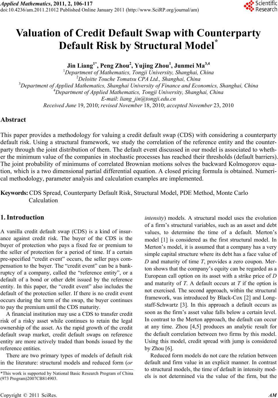
Paper Menu >>
Journal Menu >>
 Applied Mathematics, 2011, 2, 106-117 doi:10.4236/am.2011.21012 Published Online January 2011 (http://www.SciRP.org/journal/am) Copyright © 2011 SciRes. AM Valuation of Credit Default Swap with Counterparty Default Risk by Structural Model* Jin Liang1*, Peng Zhou2, Yujing Zhou1, Junmei Ma3,4 1Department of Mathematics, Tongji University, Shanghai, China 2Deloitte Touche Tomatsu CPA Ltd., Shanghai, China 3Department of Applied Mathematics, Shanghai University of Finance and Economics, Shanghai, China 4Department of Applied Mathematics, Tongji University, Shanghai, China E-mail: liang_jin@tongji.edu.cn Received June 19, 201 0; revised November 18, 2010; accepted November 23, 2010 Abstract This paper provides a methodology for valuing a credit default swap (CDS) with considering a counterparty default risk. Using a structural framework, we study the correlation of the reference entity and the counter- party through the joint distribution of them. The default event discussed in our model is associated to wheth- er the minimum value of the companies in stochastic processes has reached their thresholds (default barriers). The joint probability of minimums of correlated Brownian motions solves the backward Kolmogorov equa- tion, which is a two dimensional partial differential equation. A closed pricing formula is obtained. Numeri- cal methodology, parameter analysis and calculation examples are implemented. Keywords: CDS Spread, Counterparty Default Risk, Structural Model, PDE Method, Monte Carlo Calculation 1. Introduction A vanilla credit default swap (CDS) is a kind of insur- ance against credit risk. The buyer of the CDS is the buyer of protection who pays a fixed fee or premium to the seller of protection for a period of time. If a certain pre-specified “credit event” occurs, the seller pays com- pensation to the buyer. The “credit event” can be a bank- ruptcy of a company, called the “reference entity”, or a default of a bond or other debt issued by the reference entity. In this paper, the “credit event” also includes the default of th e protection seller. If ther e is no credit event occurs during the term of the swap, the buyer continues to pay the premium until th e CDS maturity. A financial institution may use a CDS to transfer credit risk of a risky asset while continues to retain the legal ownership of the asset. As the rapid growth of the credit default swap market, credit default swaps on reference entity are more actively traded than bonds issued by the reference entities. There are two primary types of models of default risk in the literature: structural models and reduced form (or intensity) models. A structural model uses the evolution of a firm’s structural variables, such as an asset and debt values, to determine the time of a default. Merton’s model [1] is considered as the first structural model. In Merton’s model, it is assumed that a company has a very simple capital structure where its debt has a face value of D and maturity of time T, provides a zero coupon. Mer- ton shows that the company’ s equity can be regarded as a European call option on its asset with a strike price of D and maturity of T. A default occurs at T if the option is not exercised. The second approach, within the structural framework, was introduced by Black-Cox [2] and Long- staff-Schwartz [3]. In this approach a default occurs as soon as the firm’s asset value falls below a certain level. In contrast to the Merton approach, the default can occur at any time. Zhou [4,5] produces an analytic result for the default correlation between two firms by this model. Using this model, credit spread with jump is considered by Zhou [6]. Reduced form models do not care the relation between default and firm value in an explicit manner. In contrast to structural models, th e time of default in intensity mod- els is not determined via the value of the firm, but the *This work is supported by National Basic Research Program of China (973 Program )2007CB814903. 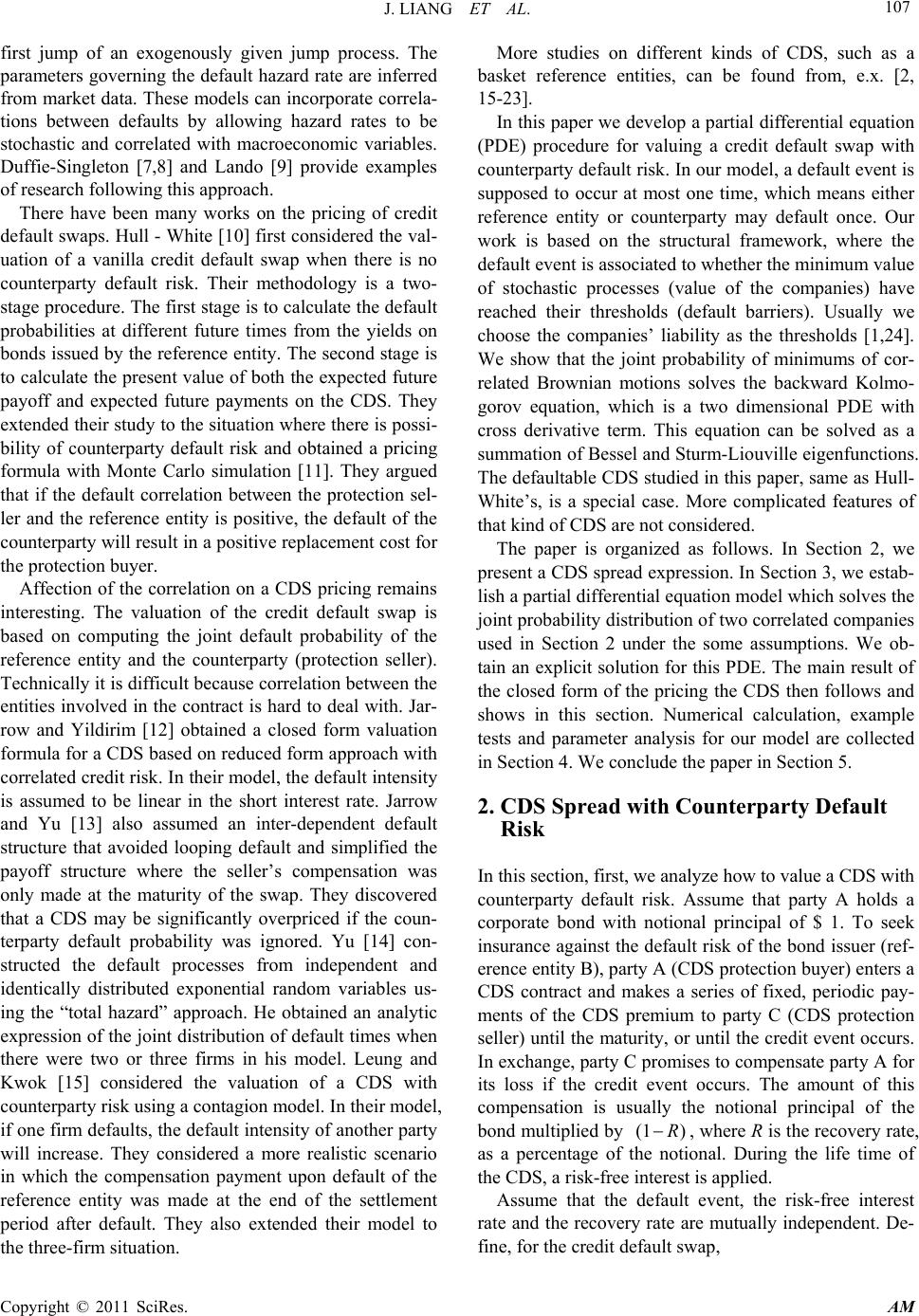 J. LIANG ET AL. Copyright © 2011 SciRes. AM 107 first jump of an exogenously given jump process. The parameters governing the default hazard rate are inferred from market data. These models can incorporate correla- tions between defaults by allowing hazard rates to be stochastic and correlated with macroeconomic variables. Duffie-Singleton [7,8] and Lando [9] provide examples of research following this approach. There have been many works on the pricing of credit default swaps. Hull - Wh ite [10] first considered the va l- uation of a vanilla credit default swap when there is no counterparty default risk. Their methodology is a two- stage procedure. The first stage is to calculate the default probabilities at different future times from the yields on bonds issued by the referen ce entity. The second stage is to calculate the present valu e of both the expected future payoff and expected future payments on the CDS. They extended their study to the situation where there is possi- bility of counterparty default risk and obtained a pricing formula with Monte Carlo simulation [11]. They argued that if the default correlation between the protection sel- ler and the reference entity is positive, the default of the counterparty will result in a positiv e replacement cost fo r the protection buyer. Affection of the correlation on a CDS pricing remains interesting. The valuation of the credit default swap is based on computing the joint default probability of the reference entity and the counterparty (protection seller). Technically it is difficult because correlation b etween the entities involved in the contract is hard to deal with. Jar- row and Yildirim [12] obtained a closed form valuation formula for a CDS based on reduced form approach with correlated credit risk. In their model, the default intens ity is assumed to be linear in the short interest rate. Jarrow and Yu [13] also assumed an inter-dependent default structure that avoided looping default and simplified the payoff structure where the seller’s compensation was only made at the maturity of the swap. They discovered that a CDS may be significantly overpriced if the coun- terparty default probability was ignored. Yu [14] con- structed the default processes from independent and identically distributed exponential random variables us- ing the “total hazard” approach. He obtained an analytic expression of the joint distribution of default times when there were two or three firms in his model. Leung and Kwok [15] considered the valuation of a CDS with counterparty risk using a contagion model. In their model, if one firm defaults, the default intensity of an other party will increase. They considered a more realistic scenario in which the compensation payment upon default of the reference entity was made at the end of the settlement period after default. They also extended their model to the three-firm situation. More studies on different kinds of CDS, such as a basket reference entities, can be found from, e.x. [2, 15-23]. In this paper we develop a partial differential equation (PDE) procedure for valuing a credit default swap with counterparty default risk. In our model, a default event is supposed to occur at most one time, which means either reference entity or counterparty may default once. Our work is based on the structural framework, where the default event is asso ciated to whether the min imum value of stochastic processes (value of the companies) have reached their thresholds (default barriers). Usually we choose the companies’ liability as the thresholds [1,24]. We show that the joint probability of minimums of cor- related Brownian motions solves the backward Kolmo- gorov equation, which is a two dimensional PDE with cross derivative term. This equation can be solved as a summation of Bessel and Sturm-Liouville eig enfunctions. The defaultable CDS studied in this paper, sa me as Hull- White’s, is a special case. More complicated features of that kind of CDS are not considered. The paper is organized as follows. In Section 2, we present a CDS spread expression. In Section 3, we estab- lish a partial differential equation model wh ich so lves the joint probability distribu tion of two correlated companies used in Section 2 under the some assumptions. We ob- tain an explicit solu tion for this PDE. The main result of the closed form of the pricing the CDS then follows and shows in this section. Numerical calculation, example tests and parameter analysis for our model are collected in Section 4. We conclude the paper in Section 5. 2. CDS Spread w ith Counterparty Default Risk In this section, first, we analyze how to value a CDS with counterparty default risk. Assume that party A holds a corporate bond with notional principal of $ 1. To seek insurance against the default risk of the bond issuer (ref- erence entity B), party A (CDS protection buyer) enters a CDS contract and makes a series of fixed, periodic pay- ments of the CDS premium to party C (CDS protection seller) until the maturity, or un til the credit event occurs. In exchang e, party C promises to compensate party A for its loss if the credit event occurs. The amount of this compensation is usually the notional principal of the bond multiplied by (1 )R , where R is the recovery rate, as a percentage of the notional. During the life time of the CDS, a risk-free interest is applied. Assume that the default event, the risk-free interest rate and the recovery rate are mutually independent. De- fine, for the credit default swap, 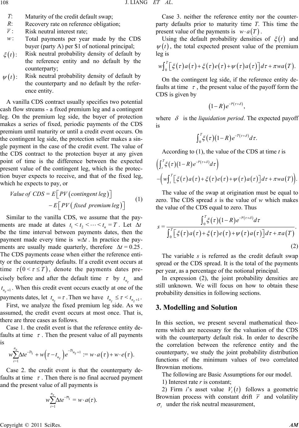 J. LIANG ET AL. Copyright © 2011 SciRes. AM 108 T: Maturity of the credit default swap; R: Recovery rate on reference obligation; :r Risk neutral interest rate; :w Total payments per year made by the CDS buyer (party A) per $ 1 of noti onal p ri ncipal ; :t Risk neutral probability density of default by the reference entity and no default by the counterparty; :t Risk neutral probability density of default by the counterparty and no default by the refer- ence entity. A vanilla CDS contract usually specifies two potential cash flow streams - a fixed premium leg and a contingent leg. On the premium leg side, the buyer of protection makes a series of fixed, periodic payments of the CDS premium until maturity or until a cred it event occurs. On the contingent leg side, the protection seller makes a sin- gle payment in the case of the credit event. The value of the CDS contract to the protection buyer at any given point of time is the difference between the expected present value of the contingent leg, which is the protec- tion buyer expects to receive, and that of the fixed leg, which he e x pects to pay , o r = Value ofCDSEPVcontingentleg EPVfixedpremium leg (1) Similar to the vanilla CDS, we assume that the pay- ments are made at dates 12 <<<= n tt tT. Let t be the time interval between payments dates, then the payment made every time is wt. In practice the pay- ments are usually made quarterly, therefore =0.25t. The CDS payments cease when either the reference enti- ty or the counterparty defaults. If a credit event occurs at time 0< T , denote the payments dates pre- cisely before and after the default time by n t and 1n t . When this credit event occurs exactly at one of the payments dates, let n t . Then we have 1 < nn tt . First, we analyze the fixed premium leg side. As we assumed, the credit event occurs at most once. That is, there are three cases as follows. Case 1. the credit event is that the reference entity de- faults at time . Then the pr esent value of all payments is 1 =1 := . nrt rt n i n i wtew tewawe Case 2. the credit event is that the counterparty de- faults at time . Then there is no final accrued payment and the present value of all payments is =1 =(). n rti i wte wa Case 3. neither the reference entity nor the counter- party defaults prior to maturity time T. This time the present value of the payments is waT. Using the default probability densities of t and t , the total expected present value of the premium leg is 0. T wa eadwaT On the contingent leg side, if the reference entity de- faults at time , the present value of the payoff form the CDS is given by 1, r Re where is the liquidation period. The expecte d payoff is 01. Tr Re d According to (1), the value of the CDS at time t is 1 . Tr t T t Re d wa eadwaT The value of the swap at origination must be equal to zero. The CDS spread s is the value of w which makes the value of the CDS equal to zero. Thus 0 0 1 =. Tr T Re d s ae adaT (2) The variable s is referred as the credit default swap spread or the CDS spread. It is the total of the payments per year, as a percentage of the notional principal. In expression (2), the joint probability densities are still unknown. We will focus on how to obtain these probability densities in following sections. 3. Modelling and Solution In this section, we present several mathematical theo- rems which are necessary for the valuation of the CDS with the counterparty default risk. In order to describe the correlation between the reference entity and the counterparty, we study the joint probability distribution functions of the minimum values of two correlated Brownian motions. The following are Basic Assumptions for our model. 1) Interest rate r is constant; 2) Firm i’s asset value i Vt follows a geometric Brownian process with constant drift r and volatility i under the risk neutral measurement, 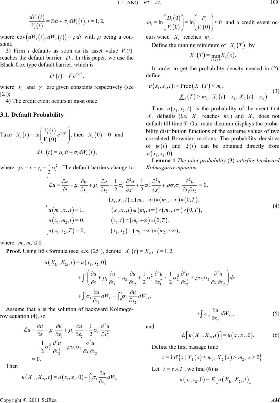 J. LIANG ET AL. Copyright © 2011 SciRes. AM 109 =, =1,2, i ii i dV trdtdW ti Vt where 12 cov ,=dW tdWtdt with being a con- stant; 3) Firm i defaults as soon as its asset value () i Vt reaches the default barrier i D. In this paper, we use the Black-Cox type default barrier, which is =, t i ii Dt Fe where i F and i are given constants respectively (see [2]); 4) The credit event occurs at most once. 3.1. Default Probability Take =ln 0 t ii i i Vt Xt e V , then 0=0 i X and =, iiii dXtdtdW t where 2 1 =2 iii r . The default barriers change to 0 =ln =ln0 00 ii i ii DF mVV and a credit event oc- curs when i X reaches i m. Define the running minimum of i X T by =. min ii tsT X TXs In order to get the probability density needed in (2), define 1 12 1 221 122 ,,:=Prob< , >|=, =. ux xtXTm X TmXtxXtx (3) Thus 12 ,,ux x t is the probability of the event that 1 X defaults (i.e. 1 X reaches 1 m) and 2 X does not default till time T. Our main theorem displays th e proba- bility distribution functions of the extreme values of two correlated Brownian motions. The probability densities of t and t can be obtained directly from 12 ,,0uxx . Lemma 1 The joint probability (3) satisfies backward Kolmogorov equation 22 2 22 12 1212 22 12 12 12 12 12 1212 12 12 11 ==0, 22 ,,,,0,, ,,=1, ,,,,0,, ,,=0, uu uuuu utx xxx xx xxt mmT umxtxxtmmT uxmt 11 1212 12 ,,0,, ,,=0, ,,,, xt mT uxxTxx mm (4) where 12 ,0.mm Proof. Using Itô's formula (see, e.x. [25]), denote =, =1,2, iit XtX i 12 12 22 2 22 12 1212 22 012 12 12 112 2 00 12 ,,= ,,0 11 22 . tt t tt ss uXXtuxx uu uuuu ds sx xxx xx uu dW dW xx Assume that u is the solution of backward Kolmogo- rov equation (4), so 2 2 12 1 2 12 1 22 2 212 212 2 1 =2 1 2 =0. uu uu usx x x uu xx x Then 12121 1 01 ,,=,,0 t tt s u uXXtuxxdW x 22 02 , t s udW x (5) and 12 12 ,,= ,,0. tt EuXXtux x (6) Define the first passage time 12 12 =inf|, >, 0.sXsm Xsms Let =tT , we find (6) is 121 2 ,,0=, , tt uxx EuXXt  J. LIANG ET AL. Copyright © 2011 SciRes. AM 110 1212 12 0 1212 12 0 12121212 12 =,,,,;,,0 ,, ,,;,,0 ,, ,,;,,0, T ss T ss mm umXs pmXsxxds uX mspX msxxds uTpTxxdd (7) where 12 12 ,,;,,0 tt pX X txx is the transition probabil- ity of being at state 12 , tt X X at time t, given that it starts at 12 , x x at time 0. Notice here, the above equation is also held for 120 0 ,,, 0<<ux xttt , if only change the low limit of the integration. Because of the boundary and final-time conditions in (4), we get 12121 212 0 ,,0=,,=,,;,,0. T tt s ux xEuXXtpmXsxxds According to the definition of 12 12 ,,;,,0 s pm Xsx x defined at the end of (7), 12 ,,0ux x is the probability defined in (3) at time 0. Now, let us solve PDE (4). First, we make the following transformation to elimi- nate the drift terms. Let =Tt and 112 2 12 12 ,, =,,, axaxb ux xepx x where 21 121221 12 222 2 12 12 =,=, 11 aa 22 22 11 2211121222 11 =. 22 ba a Then 12 ,,px x satisfies 11 22 222 22 1212 22 12 12 12 12 12 11 =0, 22 ,, =, ,,=0, ,,0=0. ama xb ppp p xx xx pm xe pxm px x (8) Next, we eliminate the cross-partial derivative and normalize the Brownian motions by a suitable transfor- mation of coordinates, this idea was introduced by He etc. ([26]. Define new coordinates 1 z and 2 z as the following 112 2 1212 1 =, 1 xmx m z (9) 22 22 =. x m z (10) Then 112 21212 ,, ,, =,,qzxxzxxpxx satis- fies 112 222 22 22 12 1 2 12 1 =, 2 ,=0, ,= , ,,0=0, am azmb qqq zz qL qL e qzz (11) where 2 1 12221221 1 =,=0, =,=.L zzzLzzzz Because the boundary conditions are more conve- niently expressed in polar coordinates, we introduce ,r corresponding to 12 ,zz as 22 2 12 1 =,tan=, z rzz z (12) thus 0, 2 and obtain ,,qr satisfies 11 2 22 22 222 sin 111 =, 2 ,0,=0, ,, =, ,,0=0. am armb qqqq rr rr qr qr e qr (13) Define a new function 11 2 22 sin ,, =, am armb fr e (14) then ,, =,,,,gr qrfr solves 22 222 111 =,,, 2 ,0,=0, ,, =0, ,,0=,,0. gggg bf r rr rr gr gr grf r (15) In order to solve PDE (15), we consider the Green’s function 000 ,,;, ,Gr r of this problem, which satisfies 22 222 000 111 =, 2 ,0,=, ,=0, ,, =. GGGG rr rr Gr Gr Grr r (16) Lemma 2 The solution of PDE (16) is 0 0000 2 ,,;, ,=r Gr r  J. LIANG ET AL. Copyright © 2011 SciRes. AM 111 22 0 0 20 0 =1 0 sinsin. rr n n rr nn eI (17) Proof. We try to find separable solutions to this equa- tion in the form of ,, =,.GrM rT (18) Plugging (18) into (16), we find that 22 222 11 ,= . 2 TMMM Mr Trr rr Divide the previous equation by ,Mr T , we find 222 222 111 ==. 2, 2 TMM M TMr rr rr (19) Since the left side of (19) is a function of and the right side is a function of r and , so it must be a constant. Denote this constant by 2 2 and we have 12 2 =.TKe On the other hand, , M r satisfies equation 22 2 222 11 =0, ,0 =,=0. MM M M rr rr Mr Mr (20) This is a Sturm-Liouville problem. We try to find se- parable solutions in the form of ,=Mr RrΘ . Plugging this i nt o ( 16) we get 222 =, RR Θ rr r RR Θ (21) with boundary conditions 0= =0.RrΘRrΘ Let 2 =ΘΘ k , then Θ solves 2=0, 0= =0. ΘkΘ ΘΘ (22) It is easy to see that =sin cos.Θ A kBk Considering the boundary conditions, we have =0B and sin= 0.Ak Because Θ is non-zero solution, we know that 0A and =,=1,2,. n n kn Thus the eigenfunctions consistent with the boundary conditions are =sin,=1,2,. n n ΘCn Finally consider the radial part of the solution Rr which satisfies 2222 =0. n rRrRrk R Denoting =r , we get the standard form of Bes- sel’s equation 2 222 2 dd =0. d dn RR kR The well known fundamental solutions of this Bessel's equation is 2 =0 1 =112 iik n knin x Jx Γki Γi and cos =. lim sin pp knpk n J xpJx Yx p Since 0 kn Y diverges and we require 0R to be bounded, the solution kn Yy is not permitted. Hence the general radial part of the solution is ,=. nk n RrJr Sum up ,,nn RrΘ over n, we have ,, =1 =1 ,= =sin. nn n nn n MrR rΘ n CJr Then 2 2 =1 ,, =, =sin. nn n GrM rT n KCe Jr Because K is a constant, we can define = n A n KC . Integral the previous equation over , we obtain the general solution to PDE (16) for ,,Gr as 2 2 0=1 ,, =sin. nn n n GrAe Jrd (23) Now we try to find the coefficient n A which fit the initial condition 000 ,, =Grrr . Mul- tiply the previous equation at 0 = by sin m and integrate over , we find  J. LIANG ET AL. Copyright © 2011 SciRes. AM 112 2 0 2 00 0 sin=d. 2mm m rrAe Jr (24) Noticing the completeness relation of 0 1 d= , ss x JaxJbxx ab a multiply equation (24) by m rJ r and integrate over r 2 0 0200 2 =sin . mm rm A eJr Plugging this expression into ,,Gr (23), we get 0 0 0 2 200 =1 2 ,,= sin sin. nn n r Gr mn eJrJrd (25) Using the fact [27] that 22 22 2 4 22 0 1 =, 22 ab cx c ss s ab xeJaxJbxdxeI cc (25) can be simplified into (17). With Green’s function 000 ,,;, ,Gr r and the boundary and initial conditions, the solution of PDE (15) can be expressed as 000000000 0 00000 0 ,,=,,;,,, , ,,;,,0,,0, F F qrdGrrbfrdrd Grrf rdrd (26) where =,|0<, 0,Fr r (27) 11 2 22 ((sin)) ,, =. am armb fr e (28) Then solution of PDE (13) is ,,=,,,, .qrgrfr Returning to the original coordinates and variables 12 ,, x xt, we get 112 2 112 2 112 2 12 12 12 ,,= ,, =,, =,,, axa xbTt axaxbTt axaxbTt ux xtepx xTt eqzzTt eqrTt (29) where 1 z, 2 z, r, are defined in (9), (10) and (12). That is, we have Theorem 1 The solution of the initial boundary prob- lem (4) has a closed form solution (29) associated by (26), (14) and (17). By now, we have already obtained the probability of that company 1 defaults and company 2 does not defaults between time t and T. Change t into 0, T into t, here comes the probability between time 0 and t. In order to obtain the probability 12 ,,vx x t of that company 2 defaults and company 1 does not default, we only need to change the positions of the parameters of the two companies such as ,,,0 iiii FV in 12 ,,ux x t. Now apply our result to the spread Formula (2) when =0 . In the valuation formula of (2), what we need are the default probability density functions of and while we only have the probability functions. Therefore, we need to modify (2). In fact, notice that a and e are piecewise continuous functions and on every piece, =0,==. rr n ae teere Integrate the numerator and denominator of (2) by parts, and we have 0 0 =1 =1, Tr T rT r numeratorR ed ReT red 0 0 1 =1 1 =1 1 =1 1 = = =| T T nti ti i nti ti i nti ti i ti ti denominatorae d ad aT aed ad aT ae 1 =1 |, r nti ti i ered aaT where =,, =,,,u andv (30) for u and v are solved in this subsection. 3.2. Survival Probability 12 ()πx,x,t To calculate the credit default swap spread s, we still need to study the joint survival probability of 12 ,, x xt for 11 > x m, 22 >, x m  J. LIANG ET AL. Copyright © 2011 SciRes. AM 113 12 12 121122 ,, =Prob>,>|= ,=. xxt X TmXTmXtxXtx Same as Theorem 1, the probability of 12 ,, x xt is the solution of PDE 22 2 22 1212 12 22 12 12 12 12 12 122 2 121 1 1212 12 11 ==0, 22 ,,,,0, , ,,=0,,,0, , ,,=0,,, 0,, ,, =1,,,,, tx xxx xx xxt mmT mxtxt mT xmtxt mT xxTxx mm (31) where 12 ,0.mm In the previous section, we get the solutions to these two PDEs in the domain 12 ,,0,,mm T 22 2 22 12 1212 22 12 12 12 12 12 12 11 ==0, 22 ,,=1, ,,=0, ,, =0, uu uuuu utx xxx xx um xt uxmt ux x T (32) and 222 22 12 12 12 22 12 12 12 12 12 12 11 ==0, 22 ,,=0, ,,=1, ,, =0, vv vvvv vtxxxx xx vm xt vxm t vx x T (33) where 12 ,0.mm Compare the boundary and final conditions of PDE (31), (32), (33), the solution to (31) can be written as the linear combination of the other two 1212 12 ,,=1 ,,,,. x xtuxxt vxxt (34) Set =0t, we get the probability of which was defined in Section 2 12 =,,0=10 0.xx (35) Thus, the CDS spread (2) can be rewritten as 0 11 1 =1 1 = . || T rT r nt tt ir ii tt it i i i ReT red s aeeredaaT (36) Remark 1 It is a special case of our model that the CDS with the counterparty default when the correlation of the counterparty and reference entity are independent. Remark 2 The same method can be used to the pric- ing the CDS for a basket reference entities. In this case, the PDE model is simpler as the boundaries condition are all equal to 0. So that, it has no problem caused by the singularity near (0,0). However, if the basket has a big number of reference entities, the closed form solution of the PDE is difficult to be obtained. 3.3. Main Result Combine the previous two subsection, we obtain the all probabilities required in Formula (36). Therefore we ob- tain the main theorem of this paper presented as follows: Theorem 2 (main theorem) Under the Basic As- sumption (1)- (4), the credit default swap spread with counterparty default risk is given by (36), where, in the formula, the probability are given by (30) solving the problem (4); are solved as in the same way; is given by (35). 4. Numerical Analysis So far, we have derived the three probabilities in Section 2. With these, we can calculate the CDS spread by (29). Even though we have a so called closed or semi-closed form solution, but the calculation of the form is still not trivial. The expression of the form includes integration  J. LIANG ET AL. Copyright © 2011 SciRes. AM 114 and infinite serial, as well as a special function. The di- rect calculation is not easy to undertaken and the result is usually not satisfying. This because that the value of the integrand concentrates in a very small area and this area is moving as the change of the time t. So that, the differ- ence approximation, in general, will make the result val- ue very small. Here we introduce an algorithm of Monte Carlo method to evaluate the form (29). It sounds that there is no dif- ference from the one to calculate CDS spread by direct Monte Carlo method, however, it is really different with and without the closed form solution. We will see it in the later. Using Monte Carlo to calculate the closed form, in fact, we only need to know how to calculate the first in- tegration of the Formula (26). The steps to do it are as follows: 1) Representing the integration with the exception of the integrand. Take 20sin 000000 ,,,,Ar frcfr e as a den- sity function, where 1221 212 =1 A , c is a constant such that 20sin 0000 00 0,, =1, Ar F cd fredrd where 000 ,,fr , which is non-negative as 0, 2 , is defined in (28). By simple calculation, we obtain 112 2 22 2sin =. 1 amamb ba A cee Now rewrite the integration, E is measured respect to f : 20 000000000 0 sin 000 ,,;,,, , =,,;,, , F Ar dGrrbfrdrd b EGrre c where G is defined in (25). 2) Random numbers fetching. In our case, the three-dimensional random ,, X YZ has a joint density 000 ,,fr . We sample this random variable ,, ii i X YZ from 30,1U, for =1,2,i, in the following way: a) First, the marginal density function respect to 0 r is 22 100000 0 00 sin 0 22 =,, =sin, aA r frfr dd aA e and the marginal distribution function is 22 220 sin 0 102 2 0 sin ()= sin =1. raA u aA r F raAedu e Then generate uniform random number 1i U and set 12 2 =ln1 sin ii XUaA . b) Secondly, for given 0 = X r, the conditional density function 0 000 0 000 2 10 ,, 2 ,| ==. 1 b b fr be fr fr e The marginal density function respect to 0 is 0 20000002 0 2 |=,|= ,fr frd and its distribution function is 2 00 200 22 0 2 |= =. u Fr du Then generate uniform random number 2i U and set 22 = ii YU . c) Thirdly, the joint marginal distribution function with respect to 0 r and 0 is 2 20 12000000 0 sin 2 02 2 ,= ,, 2 =sin, aA r frfr d aA e then for given 00 =,=XrY , the conditional densi- ty function 0 000 3000 12 00 ,, |, ==, ,1 b b fr be fr fr e and its distribution function is 0 3000 1 |, =. 1 b b e Fr e Then generate uniform random number 3i U and set 3 1 =ln11b ii ZeU b . Therefore we generate the ith random sample ,, ii i X YZ with density function 000 ,,fr . 3) By the method above, obtain three-dimensional random sample ,, ii i X YZ , then replace 000 ,,r and put it into the integ rand 20sin 000 ,,;,,Ar bGr re c . For =1,2,, ,in repeat the process n times (e.g. =1000,10000n as required), then find the mean val- ue, to find approximated the expectation. It may argue that if use Monte Car lo method, why just simulate directly on the original Formula (2)? The Fig- ure 1 can answer this question. Consider practical examples. Assuming there are two companies B and C with initial values of 0=$70 B V million and 0= $100 C V million; volatilities of them are 12 ==0.2, ==0.3 BC respectively; recover rate =0.3R; correlation =0.7 ; =0 i and the de- fault barriers are $40 million and $60 million respectiv e- ly.  J. LIANG ET AL. Copyright © 2011 SciRes. AM 115 In Figure 1, method 1 means the CDS spread is ob- tained by simulating d irectly on the o riginal Formula (2 ), method 2 means the CDS spread is calculated by our closed form solution with the integral evaluated by Monte Carlo method. The method 1 is repeated 10000 times using computer time 157.6858 second, while the method 2 is repeated 1000 times using computer time 178.7021 second. We can see that the calculation by our solution converg es much faster than directly simulate the original formula. As less as 1/10 times, the result of the method 2 is much better than the method 1. Now use the closed form solution, by Monte Carlo simulate 1000 times to calculate the integral, we can analysis the parameters of R, , and T respectively. The other parameters are chosen as above. The left figure and the right one show the impact of correlation coefficient , maturity time T and recovery rate R on CDS spread. Two figures in Figure 2 show their relationship. In the upper figure of Figure 2, CDS spreads are greater for swaps with longer maturities. The lower one illustrat e s the extent to which CDS spreads depend on the recovery rate. When the recovery rate becomes larger, the payoff will get smaller. Hence the CDS spread is getting smaller when recovery rate getting larger. Both of them show that the spread goes down as the correlation goes up. Figure 3 confirms that CDS spread increases with ex- pired time T and decreases with recover rate R, when the correlation is fixed. Figure 4 show what kind of the rules for the volatili- ties of the two companies. The behaviors of them affect to the CDS spread in different way. Suppose that the other parameters are fixed. If the volatility of the Com- pany B is larger, which means the probability of the de- fault goes larger as well, it results that the CDS spread is more expansive. On the other hand, if the volatility o f the Company C is larger, which means the probability o f the failure of the CDS payoff is larger, it results CDS spread is cheaper. Figure 1. CDS spread with counterparty risk by two me- thods. Figure 2. CDS spread with counterparty risk vs. correlation ρ, varying T (upper) and R (lower). Figure 3. CDS spread with counterparty risk vs. time T, varying R. Figure 5 is a three-dimensional surface of the value for the probability of 0,0,0 =5 BC T uV V respect to 0 B V and 0 C V. 5. Conclusions In this paper, we have introduced a PDE methodology for modeling default correlations. We assume that the value of companies follow correlated geometric brownian motions. When the asset value of a company reaches a predefined barrier, a credit event called default occurs.  J. LIANG ET AL. Copyright © 2011 SciRes. AM 116 Figure 4. CDS spread with counterparty risk vs. time T, varying 1 σ (upper) and 2 σ (lower). Figure 5. is a three-dimensional surface of the value for the probability of 0,0,0 =5 BC T uV V respect to 0 B V and 0 B V. The essential part is to derive the joint default proba- bility as the solution to a partial differential equation. This solution is more computationally efficient than tra- ditional simulation for original formula or lattice tech- niques to the equation. We applied the default probabili- ties solved from the PDE to the valuation of credit de- fault swaps with counterparty default risk. The model can be extended to the valuation of any credit derivative when the payoff is base d o n de faul t s by tw o companies. The shortage of the model is limited by the dimension, it is difficult to extend the method to a basket CDS with a large portfolio. 6. Acknowledgements The authors would like to express the thanks to Prof. Lishang Jiang for the helpful discussions and sugges- tions. 7. References [1] R. Merton, “On the Valuing of Corporate Debt: The Risk Structure of Interest Rates,” Journal of Finance, Vol. 29, No. 2, 1974, pp. 449-470. doi:10.2307/2978814 [2] F. Black and J. Cox, “Valuing Corporate Securities: Some Effects of Bond Indenture Provisions,” Journal of Finance, Vol. 31, No. 2, 1976, pp. 351-367. doi:10.2307/ 2326607 [3] F. Longstaff and E. Schwartz, “A Simple Approach to Valuing Risky Fixed and Floating Rate Debt,” Journal of Finance, Vol. 50, No. 3, 1995, pp. 789-819. doi:10.2307/ 2329288 [4] C. Zhou, “A Jump-Diffusion Approach to Modeling Cre- dit Risk and Valuing Defaultable Securities,” Finance and Economics Discussion Series, Working Paper, Board of Governors of the Federal Reserve System, Washington DC, 1997. [5] C. Zhou, “An Analysis of Default Correlation and Mul- tiple Defaults,” Review of Finance Studies, Vol. 14, No. 2, 2001, pp. 555-576. doi:10.1093/rfs/14.2.555 [6] C. Zhou, “The Term Structure of Credit Spreads with Jump Risk,” Journal of Banking & Finance, Vol. 25, No. 11, 2001, pp. 2015-2040. doi:10.1016/S0378-4266(00)00 168-0 [7] D. Duffie and K. J. Singleton, “Modeling Term Struc- tures of Defaultable Bonds,” Review of Financial Studies, Vol. 12, No. 4, 1999, pp. 687-720. doi:10.1093/rfs/12.4. 687 [8] D. Duffie and K. J. Singleton, “Credit Risk,” Princeton University Press, Princeton, 2003. [9] D. Lando, “On Cox Processes and Credit Risky Securi- ties,” Review of Derivatives Research, Vol. 2, No. 2-3, 1998, pp. 99-120. doi:10.1007/BF01531332 [10] J. Hull and A. White, “Valuing Credit Default Swaps I: No Counterparty Default Risk,” Journal of Derivatives, Vol. 8, No. 1, 2000, pp. 29-40. doi:10.3905/jod.2000. 319115 [11] J. Hull and A. White, “Valuing Credit Default Swaps II: Modeling Default Correlations,” Journal of Derivatives, Vol. 8, No. 3, 2001, pp. 12-22. doi:10.3905/jod.2001. 319153 [12] R. Jarrow and Y. Yildirim, “A Simple Model for Valuing Default Swaps when Both Market and Credit Risk are  J. LIANG ET AL. Copyright © 2011 SciRes. AM 117 Correlated,” Journal of Fixed Income, Vol. 11, No. 4, 2002, pp. 7-19. doi:10.3905/jfi.2002.319308 [13] R. Jarrow and F. Yu, “Counterparty Risk and the Pricing of Defaultable Securities,” Journal of Finance, Vol. 56, No. 5, 2001, pp. 1765-1799. doi:10.1111/0022-1082.003 89 [14] F. Yu, “Correlated Defaults and the Valuation of Defaul- table Securities,” Proceedings of 2nd International Con- ference on Credit Risk, Montréal, 15-16 April 2004, pp. 1-30. [15] S. Y. Leung and Y. K. Kwok, “Credit Default Swap Val- uation with Counterparty Risk,” The Kyoto Economic Review, Vol. 74, No. 1, 2005, pp. 25-45. [16] R. Jarrow and S. M. Turnbull, “Pricing Derivatives on Financial Securities Subject to Credit Risk,” Journal of Finance, Vol. 50, No. 1, 1995, pp. 53-86. doi:10.2307/ 2329239 [17] J. Hull and A. White, “Valuation of a CDO and nth to Default CDS without Monte Carlo Simulation,” Journal of Derivatives, Vol. 12, No. 2, 2004, pp. 8-23. doi:10. 3905/jod.2004.450964 [18] J. Hull, M. Predescu and A. White, “The Relationship between Credit Default Swap Spreads, Bond Yields, and Credit Rating Announcements,” Journal of Banking & Finance, Vol. 28, No. 11, 2004, pp. 2789-2811. doi:10. 1016/j.jbankfin.2004.06.010 [19] J. Hull, M. Predescu and A. White, “The Valuation of Correlation-Dependent Credit Derivatives Using a Struc- tural Model,” Journal of Credit Risk, Vol. 6, No. 3, 2010, pp. 99-132. [20] M. Kijima and Y. Muromachi, “Credit Events and the Valuation of Credit Derivatives of Basket Type,” Review of Derivatives Research, Vol. 4, No. 1, 2000, pp. 55-79. doi:10.1023/A:1009676412322 [21] M. Kijima and Y. Muromachi, “Valuation of a Credit Swap of the Basket Type,” Review of Derivatives Re- search, Vol. 4, No. 1, 2000, pp. 81-97. doi:10.1023/A: 1009628513231 [22] M. Wise and V. Bhansali, “Correlated Random Walks and the Joint Survival Probability,” Working Paper, Cal- tech and PIMCO, pp. 1-13. [23] P. Zhou and J. Liang, “Analysis of Credit Default Swap,” Applied Mathematics-JCU, Vol. 22, 2007, pp. 311-314. [24] K. Giesecke and L. R. Goldberg, “The Market Price of Credit Risk,” Working Paper, Cornell University, New York, 2003, pp. 1-29. [25] J. Hull, “Options, Futures and Other Derivatives,” 7th Edition, Prentice Education, Upper Saddle River, 2009. [26] H. He, P. W. Keirstead and J. Rebholz, “Double Look- backs,” Mathematical Finance, Vol. 8, No. 3, 1998, pp. 201-228. doi:10.1111/1467-9965.00053 [27] I. S. Gradshteyn and I. M. Ryzhik, “Table of Integrals, Series, and Products,” Academic Press, New York, 1980. |