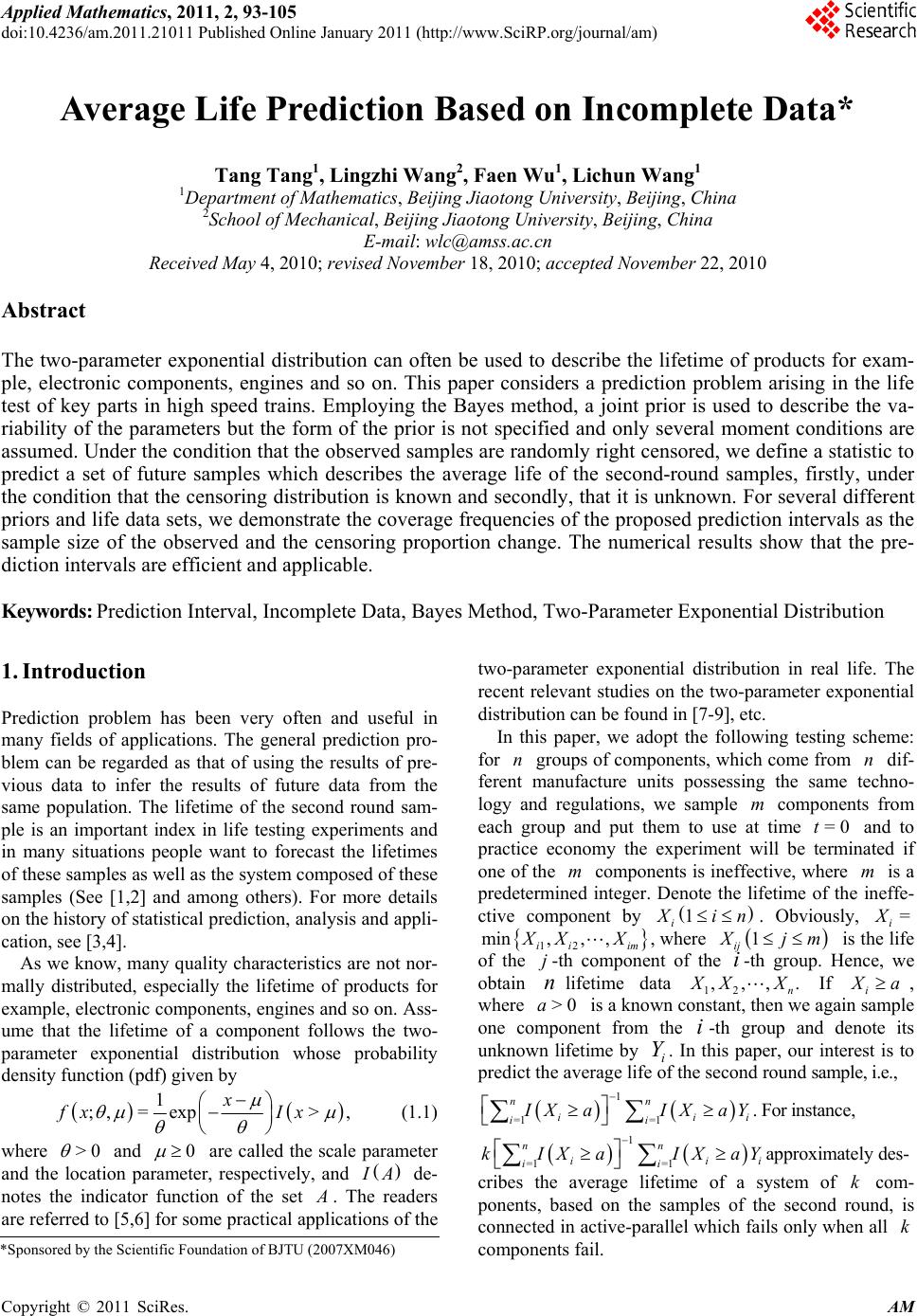Applied Mathematics, 2011, 2, 93-105
doi:10.4236/am.2011.21011 Published Online January 2011 (http://www.SciRP.org/journal/am)
Average Life Prediction Based on Incomplete Data*
Tang Tang1, Lingzhi Wang2, Faen Wu1, Lichun Wang1
1Department of Mat hem at ic s, Beijing Jiaotong University, Beijing, China
2School of Mechanical, Beijing Jiaotong University, Beijing, China
Received May 4, 2010; revised November 18, 2010; accepted November 22, 2010
Abstract
The two-parameter exponential distribution can often be used to describe the lifetime of products for exam-
ple, electronic components, engines and so on. This paper considers a prediction problem arising in the life
test of key parts in high speed trains. Employing the Bayes method, a joint prior is used to describe the va-
riability of the parameters but the form of the prior is not specified and only several moment conditions are
assumed. Under the condition that the observed samples are randomly right censored, we define a statistic to
predict a set of future samples which describes the average life of the second-round samples, firstly, under
the condition that the censoring distribution is known and secondly, that it is unknown. For several different
priors and life data sets, we demonstrate the coverage frequencies of the proposed prediction intervals as the
sample size of the observed and the censoring proportion change. The numerical results show that the pre-
diction intervals are efficient and applicable.
Keywords: Prediction Interval, Incomplete Data, Bayes Method, Two-Parameter Exponential Distribution
1. Introduction
Prediction problem has been very often and useful in
many fields of applications. The general prediction pro-
blem can be regarded as that of using the results of pre-
vious data to infer the results of future data from the
same population. The lifetime of the second round sam-
ple is an important index in life testing experiments and
in many situations people want to forecast the lifetimes
of these samples as well as the system composed of these
samples (See [1,2] and among others). For more details
on the history of statistical prediction, analysis and appli-
cation, see [3,4].
As we know, many quality characteristics are not nor-
mally distributed, especially the lifetime of products for
example, electronic components, engines and so on. Ass-
ume that the lifetime of a component follows the two-
parameter exponential distribution whose probability
density funct i o n (p df) given by
 
1
;,= exp>,
x
fx Ix








 (1.1)
where >0

and 0

 are called the scale parameter
and the location parameter, respectively, and


I
A de-
notes the indicator function of the set
A
. The readers
are referred to [5,6] for some practical applications of the
two-parameter exponential distribution in real life. The
recent relevant studies on the two-parameter exponential
distribution can be found in [7-9], etc.
In this paper, we adopt the following testing scheme:
for n groups of components, which come from n dif-
ferent manufacture units possessing the same techno-
logy and regulations, we sample m components from
each group and put them to use at time =0t and to
practice economy the experiment will be terminated if
one of the m components is ineffective, where m is a
predetermined integer. Denote the lifetime of the ineffe-
ctive component by


1
i
X
in . Obviously, =
i
X


12
min,, ,,
ii im
XX Xwhere  1
ij
X
jm is the life
of the j-th component of the i-th group. Hence, we
obtain nlifetime data 12 ,,,.
n
X
XX If i
X
a,
where >0a is a known constant, then we again sample
one component from the i-th group and denote its
unknown lifetime by i Y. In this paper, our interest is to
predict the av erage life of the second round sample, i .e.,
 
1
=1 =1
nn
iii
ii
I
Xa IXaY





. For i nstance,
 
1
=1 =1
nn
iii
ii
kIXa IXaY





approximately des-
cribes the average lifetime of a system of k com-
ponents, based on the samples of the second round, is
connected in active-parallel which fails on ly when all k
components fail.
*Sponsored by the Scientific Foundation of BJTU (2007XM046)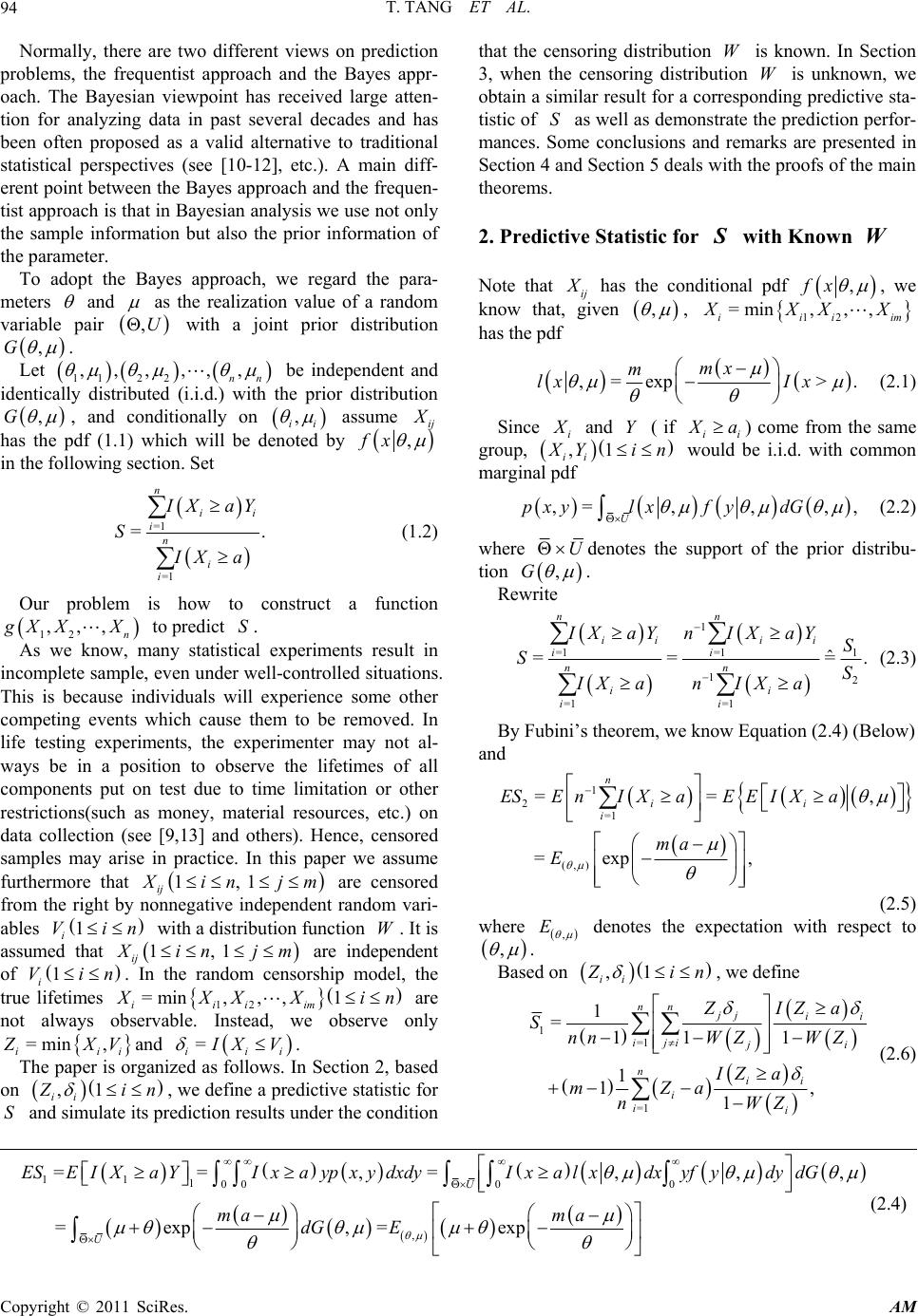

T. TANG ET AL. 94
Normally, there are two different views on prediction
problems, the frequentist approach and the Bayes appr-
oach. The Bayesian viewpoint has received large atten-
tion for analyzing data in past several decades and has
been often proposed as a valid alternative to traditional
statistical perspectives (see [10-12], etc.). A main diff-
erent point between the Bayes approach an d the frequen-
tist approach is that in Bayesian analysis we use not on ly
the sample information but also the prior information of
the parameter.
To adopt the Bayes approach, we regard the para-
meters

and

as the realization value of a random
variable pair  ,U with a joint prior distribution

,G

.
Let
  
112 2
,,,,,,
nn

   be independent and
identically distributed (i.i.d.) with the prior distribution

,G

, and conditionally on

,
ii

 assume ij
X
has the pdf (1.1) which will be denoted by


,fx

in the following section. Set


=1
=1
=.
n
ii
in
i
i
I
XaY
S
I
Xa



 (1.2)
Our problem is how to construct a function

12
,,,
n
g
XX X to predict S.
As we know, many statistical experiments result in
incomplete sample, even under well-controlled situations.
This is because individuals will experience some other
competing events which cause them to be removed. In
life testing experiments, the experimenter may not al-
ways be in a position to observe the lifetimes of all
components put on test due to time limitation or other
restrictions(such as money, material resources, etc.) on
data collection (see [9,13] and others). Hence, censored
samples may arise in practice. In this paper we assume
furthermore that 
1, 1
ij
X
in jm  are censored
from the right by nonnegative independent random vari-
ables

1
i
Vin with a distribution function W. It is
assumed that  1, 1
ij
X
in jm  are independent
of

1
i
Vin . In the random censorship model, the
true lifetimes



12
=min,, ,1
iiiim
X
XX Xin are
not always observable. Instead, we observe only

=min ,
iii
Z
XVand

=
iii
I
XV  .
The paper is organized as follows. In Section 2, based
on



,1
ii
Z
in   , we define a predictive statistic for
S and simulate its prediction results under the condition
that the censoring distribution W is known. In Section
3, when the censoring distribution W is unknown, we
obtain a s imilar result for a co rresponding predictive sta-
tistic of S as well as demonstrate the prediction perfor-
mances. Some conclusions and remarks are presented in
Section 4 and Section 5 deals with the proofs of the main
theorems.
2. Predictive Statistic for
S
with Known W
Note that ij
X
has the conditional pdf 

,fx

, we
know that, given

 ,

,

12
=min,, ,
iiiim
XXXX
has the pdf



,=exp >.
mx
m
lx Ix

 





(2.1)
Since i
X
and Y ( if ii
X
a) come from the same
group,




,1
ii
X
Yin

 would be i.i.d. with common
marginal pdf




 ,=,, ,,
U
pxylxf ydG






 (2.2)
where U

denotes the support of the prior distribu-
tion

 ,G

.
Rewrite




1
=1=1 1
12
=1 =1
ˆ == =.
nn
ii ii
ii
nn
ii
ii
IX aY nIX aYS
SS
IX anIXa





 (2.3)
By Fubini’s theorem, we know Equation (2.4) (Below)
and
  


1
2=1
(,)
==,
=exp,
n
ii
i
ESEnIXaEEI Xa
ma
E












 

 




(2.5)
where

,
E


denotes the expectation with respect to


,

.
Based on




,1
ii
Z
in 

, we define








1=1
=1
1
=11 1
1
1,
1
nn jj ii
iji ji
nii
i
ii
ZIZ a
SnnWZWZ
IZ a
mZa
nWZ







 



 


(2.6)




 

  

 
11
1000 0
,
== ,=,,,
=exp,=exp
U
U
ESE I XaYI xaypxydxdyI xalxdxyfydydG
ma ma
dG E




 

 



 
 


  
 
  
 

 
(2.4)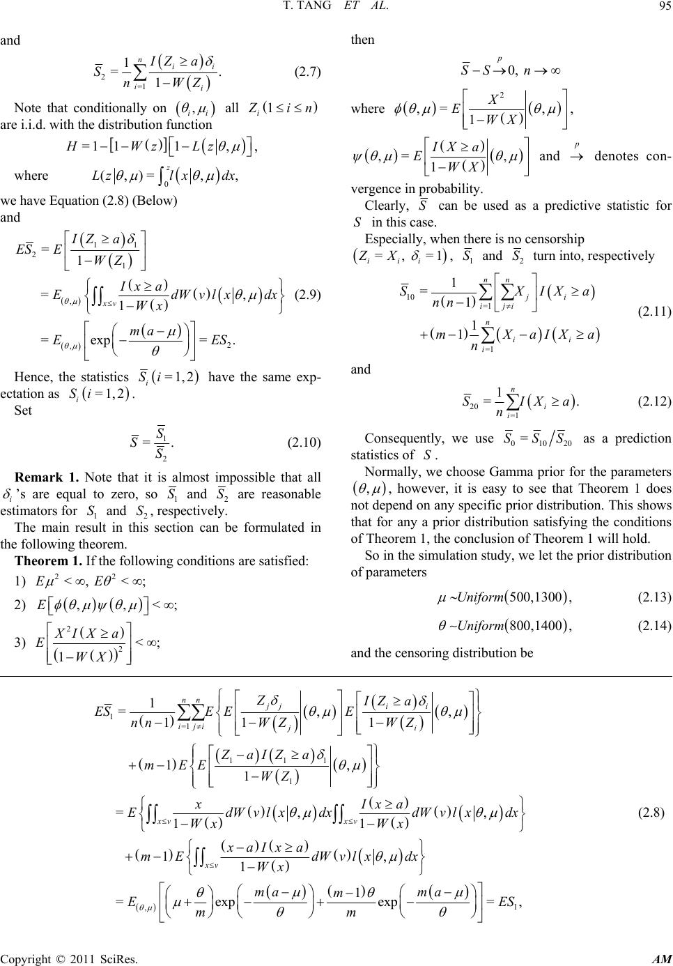

T. TANG ET AL. 95
and


2=1
1
=.
1
nii
ii
IZ a
SnWZ



 (2.7)
Note that conditionally on


,
ii

 all

1
i
Z
in


are i.i.d. with the distribution function
 


=1 11,HWzLz




 

,
where

0
(,)=,,
z
Lzl xdx  

we have Equation (2.8) (B elow)
and




 



11
21
,
2 ,
=1
=,
1
=exp=.
xv
IZa
ES EWZ
Ix a
EdWvlxdx
Wx
ma
EES












 




 

 


 (2.9)
Hence, the statistics  =1,2
i
Si have the same exp-
ectation as
 =1,2
i
Si .
Set
1
2
=.
S
SS (2.10)
Remark 1. Note that it is almost impossible that all
i

’s are equal to zero, so 1 S and 2 S are reasonable
estimators for 1 S and 2 S, respectively.
The main result in this section can be formulated in
the following theorem.
Theorem 1. If the following conditions are satisfied:
1) 22 <, <;EE  
2)  ,,<;E  

3)



2
2<;
1
XIXa
EWX






then
0,
p
SS n


where 


2
,= ,
1
X
EWX

 








,




,= ,
1
IX a
EWX












 and
p
 denotes con-
vergence in probability.
Clearly, S can be used as a predictive statistic for
S in this case.
Especially, when there is no censors hip


=, =1
iii
ZX  , 1 S and 2 S turn into, respectively




10 =1
=1
1
=1
1
1
nn
ji
iji
n
ii
i
SXIXa
nn
mXaIXa
n

 






(2.11)
and

20 =1
1
=.
n
i
i
SIXa
n
 (2.12)
Consequently, we use 01020 =SSS as a prediction
statistics of S.
Normally, we choose Gamma prior for the parameters

 ,

, however, it is easy to see that Theorem 1 does
not depend on any specific prior distribution. This shows
that for any a prior distribution satisfying the conditions
of Theorem 1, the conclusion of Theorem 1 will hold.
So in the simulation study, we let the prior distribution
of parameters

 500,1300 ,Uniform   (2.13)

 800,1400 ,Uniform   (2.14)
and the censoring distribution be










 


 


1=1
111
1
1
=,,
11 1
1,
1
=,,
11
1
nn jj ii
iji ji
xv xv
xv
ZIZ a
ESE EE
nnWZ WZ
ZaIZa
mEE WZ
xIxa
EdWv lxdxdWv lxdx
Wx Wx
mE

 

 











 










 












 


 





1
,
,
1
1
=expexp=,
xaIxa
dWv lxdx
Wx
ma ma m
EES
mm


 

 




   

 
 



(2.8)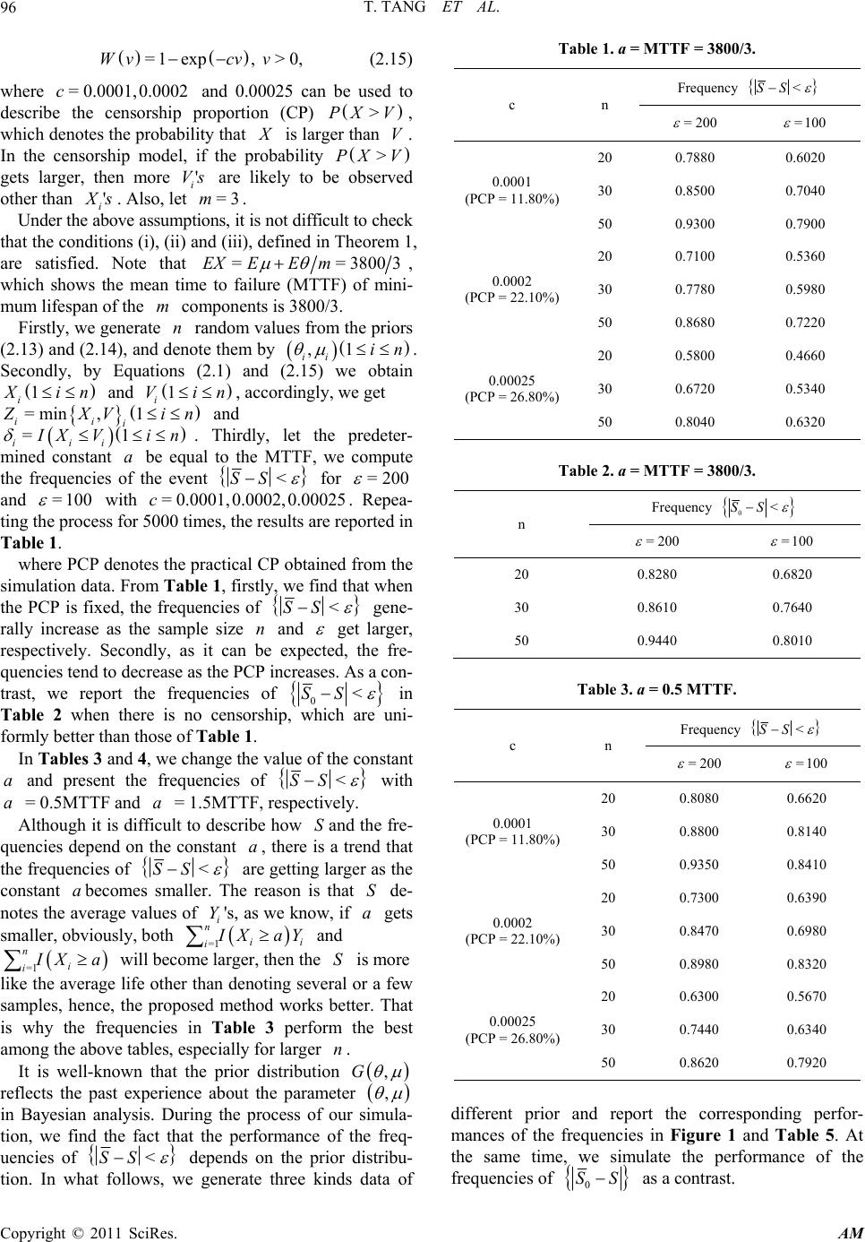

T. TANG ET AL. 96
 
=1exp, >0,Wvcv v (2.15)
where = 0.0001,0.0002c and 0.00025 can be used to
describe the censorship proportion (CP)


>PXV,
which denotes the probability that
X
is larger than V.
In the censorship model, if the probability


>PX V
gets larger, then more '
i
Vs are likely to be observed
other than '
i
X
s. Also, let =3m.
Under the above assumptions, it is not difficult to check
that the conditions (i), (ii) and (iii), defined in Theorem 1,
are satisfied. Note that ==38003EXEE m

 ,
which shows the mean time to failure (MTTF) of mini-
mum lifespan of the m components is 3800/3.
Firstly, we generate n random values from the priors
(2.13) and (2.14), and denote them by



,1
ii in


.
Secondly, by Equations (2.1) and (2.15) we obtain

1
i
X
in and

1
i
Vin , accordingly, we get



=min,1
ii
i
Z
XVin and



=1
iii
I
XV in  . Thirdly, let the predeter-
mined constant a be equal to the MTTF, we compute
the frequencies of the event


<SS

 for =200

and =100

with = 0.0001,0.0002,0.00025c. Repea-
ting the process for 5000 times, the results are reported in
Table 1.
where PCP denotes the practical CP obtained from the
simulation data. From Table 1, firstly, we find that when
the PCP is fixed, the frequencies of

<SS

 gene-
rally increase as the sample size n and

get larger,
respectively. Secondly, as it can be expected, the fre-
quencies tend to decrease as the PCP increases. As a con-
trast, we report the frequencies of

0<SS

 in
Table 2 when there is no censorship, which are uni-
formly better than those of Table 1.
In Tab les 3 and 4, we change the value of the constant
a and present the frequencies of

<SS

 with
a = 0.5MTTF and a = 1.5M T T F, res pectively.
Although it is difficult to describe how Sand the fr e-
quencies depend on the constant a, there is a trend that
the frequencies of

<SS

 are getting larger as the
constant abecomes smaller. The reason is that S de-
notes the average values of i
Y's, as we know, if a gets
smaller, obviously, both

=1
n
ii
i
I
XaY
 and

=1
n
i
i
I
Xa
 will become larger, then the S is more
like the average life other than denoting several or a few
samples, hence, the proposed method works better. That
is why the frequencies in Table 3 perform the best
among the above tables, especially for larger n.
It is well-known that the prior distribution

 ,G

reflects the past experience about the parameter

 ,

in Bayesian analysis. During the process of our simula-
tion, we find the fact that the performance of the freq-
uencies of

<SS

 depends on the prior distribu-
tion. In what follows, we generate three kinds data of
Table 1. a = MTTF = 3800/3.
c n
Frequency


<SS


= 200

=100

0.0001
(PCP = 11.80%)
20 0.7880 0.6020
30 0.8500 0.7040
50 0.9300 0.7900
0.0002
(PCP = 22.10%)
20 0.7100 0.5360
30 0.7780 0.5980
50 0.8680 0.7220
0.00025
(PCP = 26.80%)
20 0.5800 0.4660
30 0.6720 0.5340
50 0.8040 0.6320
Table 2. a = MTTF = 3800/3.
n Frequency


0<SS


=200

=100

20 0.8280 0.6820
30 0.8610 0.7640
50 0.9440 0.8010
Table 3. a = 0.5 MTTF.
c n
Frequency


<SS


=200

=100

0.0001
(PCP = 11.80%)
20 0.8080 0.6620
30 0.8800 0.8140
50 0.9350 0.8410
0.0002
(PCP = 22.10%)
20 0.7300 0.6390
30 0.8470 0.6980
50 0.8980 0.8320
0.00025
(PCP = 26.80%)
20 0.6300 0.5670
30 0.7440 0.6340
50 0.8620 0.7920
different prior and report the corresponding perfor-
mances of the frequencies in Figure 1 and Table 5. At
the same time, we simulate the performance of the
frequencies of


0
SS as a contrast.

T. TANG ET AL. 97
Table 4. a = 1.5 MTTF.
c n
Frequency


<SS


=200  =100 
0.0001
(PCP = 11.80 %)
20 0.6860 0.5920
30 0.7600 0.6060
50 0.9050 0.6800
0.0002
(PCP = 22.10 %)
20 0.6100 0.5160
30 0.6760 0.5770
50 0.7690 0.6240
0.00025
(PCP = 26.80 %)
20 0.4880 0.4260
30 0.5710 0.5130
50 0.7050 0.4650
From the above, we see that for the three different
priors of

,

, which have the same prior means for

and

, respectively, under the condition that their
PCPs are almost the same, the more concentrative the
prior values, the better the performances of the frequen-
cies. This numerical evidence means that the proposed
prediction intervals are in accordance with practice and
applicable.
3. Predictive Statistic for
S
with Unknown
W
Note that the censoring distribution (.)W is unknown,
hence the predictive statistic S is unavailable to use.
This leads us to adopt the product limit estimator, which
introduced to statistical problems by [14], to propose a
corresponding predictive statistic for S in this case.
Define
1
2
ˆ
ˆ=,
ˆ
S
SS (3.1)
where








1=1
=1
1
ˆ=ˆˆ
111
1
1,
ˆ
1
nn jj ii
iji nj ni
nii
i
ini
ZIZ a
Snn WZ WZ
IZ a
mZa
nWZ











 


(3.2)


2=1
1
ˆ=,
ˆ
1
nii
ini
IZ a
SnWZ



 (3.3)
and the product limit estimator

ˆn
Wt is given by

 


(,=0
=1
ˆ
1=, <,
1
IZ t
nii
nn
i
ni
Wtt Z
ni
 





 (3.4)
where
 

12 n
Z
ZZ

 are the order statistics of


12
,,,
n
Z
ZZ and

i

is the concomitant of

i
Z
.
Theorem 2. Under the same conditions as Theorem 1,
we have
ˆ0.
p
SS
Obviously, ˆ S can be used as a predictive statistic for
S when the censoring distribution W is unknown.
Remark 2. Note that in the case that the censoring
distribution W is unknown, it is impossible to check
whether the conditions of Theorem 2 are satisfied or not.
Hence, we first need to propose a distribution function
W to fit the data 12 ,,,
n
VV V.
Consider the following several data sets, which come
from [15]. We take them as the the censoring variables
12
,,,
n
VV V.
=5n, 381, 395, 408, 423, 431.
=20n, 350, 380, 400, 430, 450, 470, 480, 500, 520,
540, 550, 570, 600, 610, 630, 650, 670, 730, 770, 840.
=31n, 30 926, 34 554, 36 381, 38 423, 40 103, 40
501, 42 200 , 44 392, 46 092, 46 125, 46 175, 48 02 5, 48
025, 48 055 , 48 055, 48 055, 48 055, 48 056, 51 67 5, 52
344, 52 345 , 52 345, 52 345, 52 379, 55 997, 56 20 2, 57
709, 57 709, 57 709, 57 709, 63 496.
=71n, 3 95642, 4 004 18 , 4 09 161 , 4 355 05 , 4 35 54 0,
4 37601, 4 39179, 4 48768, 4 48768, 4 73667, 4 73667, 4
93985, 4 96362, 5 22019, 5 35341, 5 37272, 5 418045
44411, 5 60317, 5 69810, 5 74617, 5 84352, 6 17514, 6
19741, 6 24969, 6 27976, 6 27976, 6 57274, 6 74048, 6
88765, 7 18309, 7 20900, 7 20900, 7 20900, 7 20900, 7
36640, 7 58164, 7 58164, 7 58164, 7 64559, 8 24600, 8
5997, 8 71397, 8 93634, 9 04422, 9 197 45, 9 51173, 9
75447, 9 96745, 10 13631, 10 17288, 10 17288, 10
30804, 10 39500, 10 609 23, 10 60923, 10 78897, 10
87997, 10 97175, 11 59441, 11 99059, 12 23731, 12
40031, 12 40031, 12 55001, 13 19873, 13 94778, 15
55712, 17 646 12, 19 84823, 23 19907.
As we know the Weibu ll distrib ution is widely ap plied
to life testing and reliability analysis. Some studies on it
have been quickly developed in recent years (see [16]
and [17], etc). The cumulative distribution function
(CDF) of the three-parameter Weibull distribution is

=1 exp,
t
Ft












(3.5)
where

is the shape parameter,

is the location para-
meter and

is the scale parameter.
Employing the method proposed by [18], we use the
three-parameter Weibull distribution to fit the above four
groups data and test the fitting by Kolmogorov-Smirnov

T. TANG ET AL. 98
Figure 1. The values of


,


nn
for three different priors.
Table 5. a = 0.5 MTTF.
PCP and the prior n Frequency


<SS

 Frequency


0<SS


= 200  =100  =200  =100 
PCP=11.76%
50 0.9240 0.6730 0.9420 0.7060  500,1300U  
 800,1400U  
PCP=11.94%
50 0.9300 0.7280 0.9480 0.7520  700,1100U  
 1000,1200U  
PCP=11.91%
50 0.9370 0.7540 0.9510 0.8500  850,950U  
 1050,1150U  
s (K-S) test method. Note that (3.5) can be transformed
into the following linear equation




  lnln 1=lnln.Ft t

  (3.6)
Firstly, to estimate the location parameter

, we fol-
low the principle of gold en-section to find a value which
located in the interval



1
0,t to maximize the absolute
value of the correlation coefficient defined by


=1
22
=1 =1
=,
n
ii
i
nn
ii
ii
xxyy
xx yy






T. TANG ET AL. 99
where


=1 =1
=, =, =ln,
nn
iii
i
ii
xxnyynxt






=lnln1
ii
yFt



and (1)(2)( ) ,,,
n
tt tare the stati-
stics of 12 ,, ,
n
tt t and






=0.320.36
i
Ft in.
Secondly, adoptin g the least square method and regar-
ding every group data as 12
,, ,
n
tt t, we report the fit-
ting results and the estimators of the parameters as well
as the Kolmogorov-Smirnov test values in Figures 2-5
and Table 6. Where the K-S value denotes the
Kolmogorov-Smirnov test value.
Assume that the parameters  ,

have priors sim-
ilar to (2.13 ) and (2.14), fo r example
 
12 12
,, ,Uniform Uniform

  , and =3m.
Obviously, under the condition that the censoring distri-
bution W is Weibull distribution with the above esti-
mated parameters, it is easy to check that the conditions
of Theorem 2 are satisfied.
We simulate the frequencies of


ˆ<
SS

 as the
PCP changes and present the results in what follows.
Also, we refer to the performances of the frequencies of

0<SS

 as a contrast.
From Tables 7-9, firstly, it is the same as before, we
find that for the fixed PCP, the frequencies of


ˆ<
SS

 and

0<SS

generally increase as the
Constant a gets small. Secondly, compared with Ta-
bles 1, 3 and 4, for the same sample size n, the fre-
quencies of


<SS

 generally tend to be larger
than those of


ˆ<
SS

, which means in this case for
given

S is more concentrated in the vicinity of S.
However, this may not be the case all the time. One
reason is that i
X
’s and i V’s are different even for each
the same sample size n and hence this makes the
comparison more complicated. Thirdly, consistently,
whether W is known or not the performances of the
frequencies of


0<SS

 are the best. Also, as it can
be expected, the frequencies of


ˆ<
SS

 generally
tend to decrease as the PCP increases.
4. Conclusions and Remarks
In this paper, assume the observed lifetimes of com-
ponents are rightly censored, we define a prediction sta-
tistic to predict the average value of some untested com-
ponents, firstly, under the condition that the censoring
distribution is known and secondly, that it is unknown. In
the case that the censoring distribution is unknown, we
first fit the data 12 ,,,
n
VV V with a distribution function,
say


Wt, and test the fitting by Kolmogorov-Smirnov
Figure 2. The case of n = 5.

T. TANG ET AL. 100
Figure 3. The case of n = 20.
Figure 4. The case of n = 31.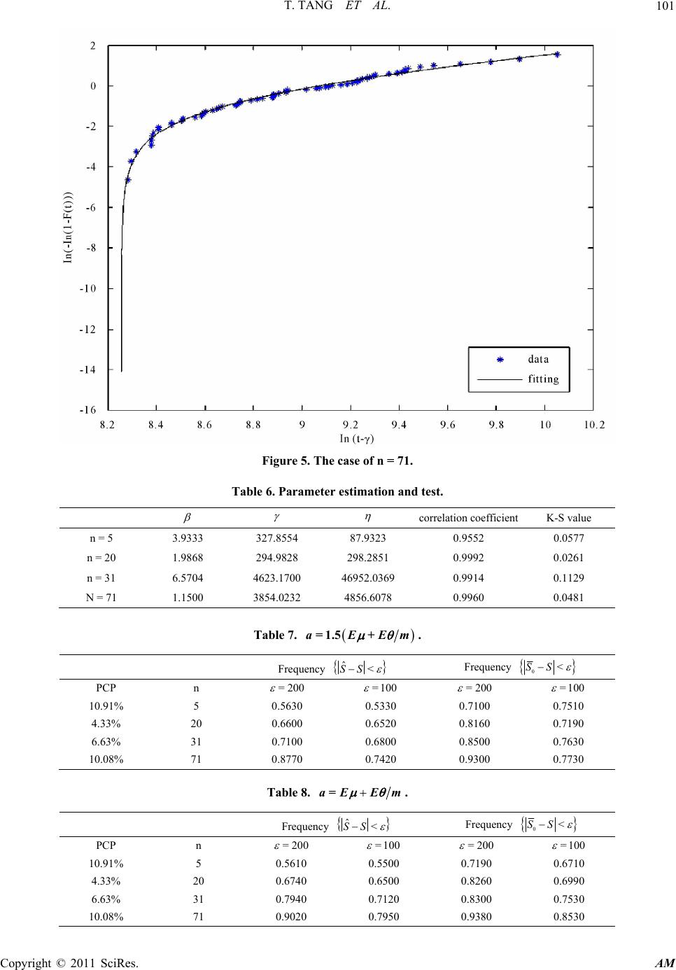

T. TANG ET AL. 101
Figure 5. The case of n = 71.
Table 6. Parameter estimation and test.



correlation coefficient K-S value
n = 5 3.9333 327.8554 87.9323 0.9552 0.0577
n = 20 1.9868 294.9828 298.2851 0.9992 0.0261
n = 31 6.5704 4623.17 00 46952.0369 0.9914 0.1129
N = 71 1.1500 3854.0232 4856.6078 0.9960 0.0481
Table 7.


=1.5 +  aEEm.
Frequency


ˆ<SS

 Frequency


0<SS


PCP n = 200

=100

=200

=100

10.91% 5 0.5630 0.5330 0.7100 0.7510
4.33% 20 0.6600 0.6520 0.8160 0.7190
6.63% 31 0.7100 0.6800 0.8500 0.7630
10.08% 71 0.8770 0.7420 0.9300 0.7730
Table 8. =  aE Em.
Frequency


ˆ<SS

 Frequency


0<SS


PCP n = 200

=100

=200

=100

10.91% 5 0.5610 0.5500 0.7190 0.6710
4.33% 20 0.6740 0.6500 0.8260 0.6990
6.63% 31 0.7940 0.7120 0.8300 0.7530
10.08% 71 0.9020 0.7950 0.9380 0.8530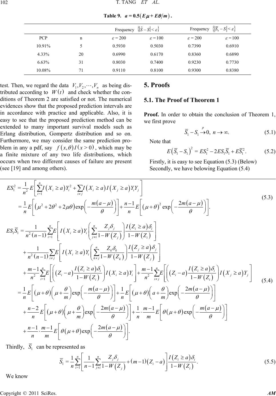

T. TANG ET AL. 102
Table 9.


=0.5+  aEEm.
Frequency


ˆ<SS

 Frequency


0<SS


PCP n = 200

=100

=200

=100

10.91% 5 0.5930 0.5030 0.7390 0.6910
4.33% 20 0.6990 0.6170 0.8360 0.6890
6.63% 31 0.8030 0.7400 0.9230 0.7730
10.08% 71 0.9110 0.8100 0.9300 0.8380
test. Then, we regard th e data 12 ,,,
n
VV V as being dis-
tributed according to


Wt and check whether the con-
ditions of Theorem 2 are satisfied or not. The numerical
evidences show that the proposed prediction in tervals are
in accordance with practice and applicable. Also, it is
easy to see that the proposed prediction method can be
extended to many important survival models such as
Erlang distribution, Gompertz distribution and so on.
Furthermore, we may consider the same prediction pro-
blem in any a pdf, say 

,>0fx Ix  , which may be
a finite mixture of any two life distributions, which
occurs when two different causes of failure are present
(see [19] and among others).
5. Proofs
5.1. The Proof of Theorem 1
Proof. In order to obtain the conclusion of Theorem 1,
we first pr ove
11
0, .
p
SS n

 (5.1)
Note that


222
11111 1
=2 .ES SESESSES (5.2)
Firstly, it is easy to see Equation (5.3) (Below)
Secondly, we have belowing Equation (5.4)
 


  
22
12=1
2
22
1
=
2
11
=22expexp.
n
ii i jij
iij
ESEI XaYI XaI XaYY
n
ma ma
n
EE
nn

 



 



 


  
 


(5.3)






 




 
11 2=1
2
2=1
1
=11
1
1
11
1
1
1
nn
jj ii
ii
iji
ji
njj
kk
ii
ijkj kj
nii
iii
ii
ZIZ a
ES SEIXaYWZ WZ
nn
IZa
Z
EIX aYWZ WZ
nn
IZ a
mEZa IXaY
WZ n









  











 






 
 












   
 
2
1
1
2 11
=expexp
2
211
exp
nii
ijj
ij i
IZ a
mEZa IXaY
WZ n
ma ma
EEa
nm nm
ma
nm
EE
nm nm

 
 



 







 

 







 
 

 
  
 
 
 
 




 
 

 


 
 
exp
2
11
exp.
ma
ma
nm
E
nm



 
















(5.4)
Thirdly, 1
S ca n be rep rese nted as





1=1
11
=1.
11 1
nn
jj ii
i
iji ji
ZIZ a
SmZa
n nWZWZ







 


 (5.5)
We know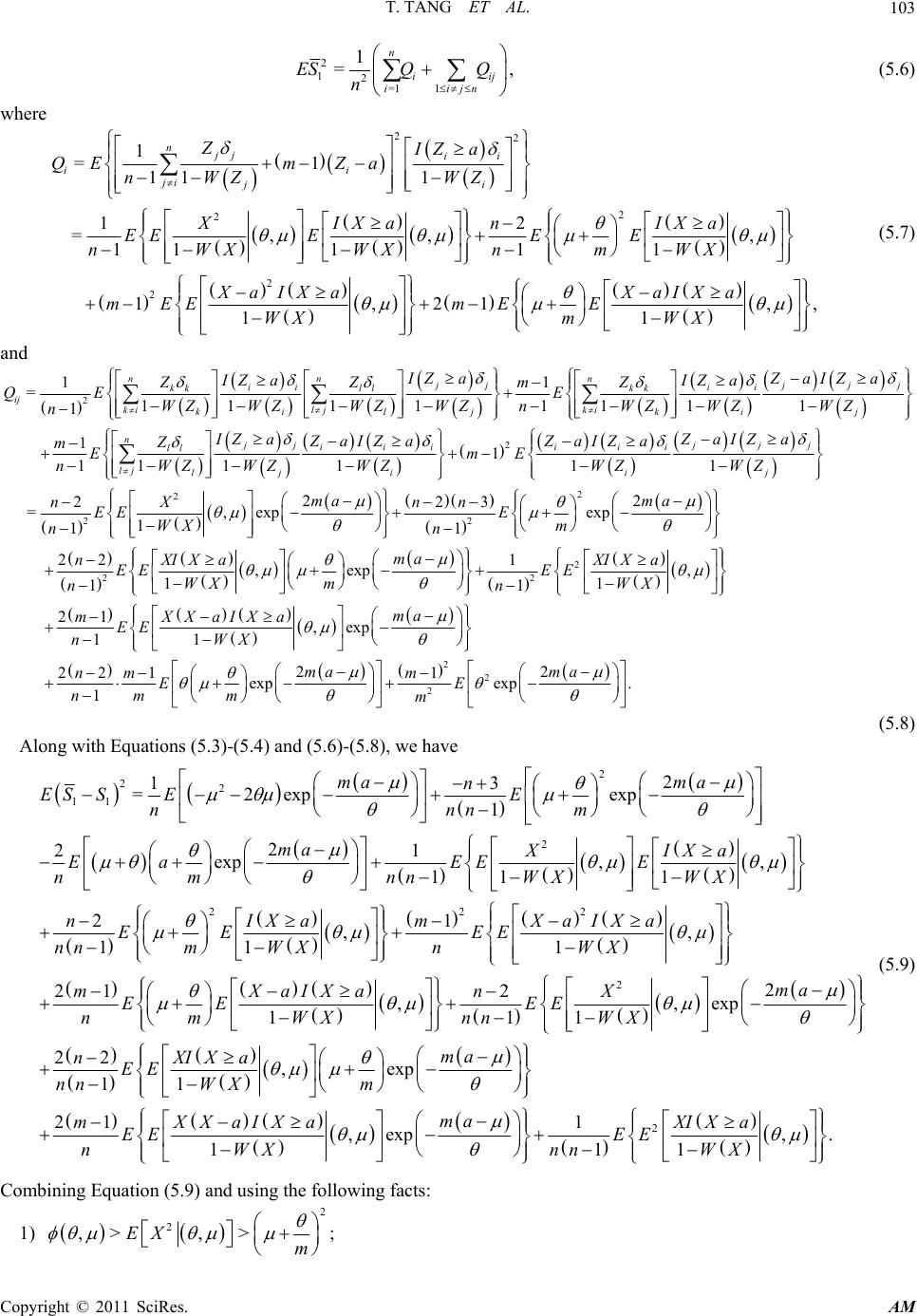

T. TANG ET AL. 103
2
12=1 1
1
=,
n
iij
iijn
ESQ Q
n 




 (5.6)
where













  


22
2
2
2
2
1
=1
11 1
12
=,,,
1111 1
1,
1
njj ii
ii
ji ji
ZIZ a
QEm Za
nWZ WZ
XIXanIXa
EEEE E
nWX WXnmWX
XaIXa
mEE WX


 







 
 
 
 
 






 
  


 
 
  



   
 


 

  


21, ,
1
XaIXa
mE E
mWX









  
 

 













(5.7)
and
 

 













2
11
=11111111
1
1
11
nn n
j
jjjj
ii ii
kk llkk
ij kil jki
kiljkij
nj
ll
lj l
IZaZ aIZa
IZ aIZ a
ZZ Z
m
QE E
WZ WZWZWZnWZ WZWZ
n
IZ a
Z
mE
nWZ



 


 



 





 

 








 











 



2
2
2
22
1
111 1
22
223
=,expexp
1
11
2
jjjj
iii iii
jii j
ZaIZa
ZaIZaZaIZa
mE
WZ WZWZWZ
ma ma
nX nn
EE E
WX m
nn
n




 



 



 


 

 

 
 
  
 
 

 






 




 

 

2
2 2
21
,exp ,
11
11
21
,exp
11
2 221
exp
1
ma
XI XaXI Xa
EE EE
WX mWX
nn
ma
mXXaIXa
EE
nWX
m nm
E
nm m
 



 



  
  
 
 
  
 
  


 


 





 




 





22
2
2 1exp. ama mE
m




   

  
 

(5.8)
Along with Equa tions (5.3)-(5.4 ) and (5.6)-(5.8), we have





 







2
22
11
2
2
2
13
=2exp exp
1
2
21
exp, ,
11 1
2
1
ma ma
n
ES SEE
nnnm
ma XIXa
EaEE E
nm nnWXWX
nIX
EE
nn m


 



 





 

 
 

  

 





 

 
 
   
   
 
 









 


 


 
 





22
2
1
,,
11
2
21 2
,,exp
111
22 ,
11
amXaIXa
EE
WX nWX
ma
mXaIXanX
EE EE
nm WXnnWX
nXIXa
EE
nnW Xm
 


 


 



















 
  

  
 
   

  
 

 











 

 




2
exp
21 1
,exp, .
111
ma
ma
mXX aIXaXIXa
EE EE
nWX nnWX



 


 


 
 



 

 



 



 

(5.9)
Combining Equation (5.9) and using the following facts:
1)
 
2
2
,>,>;EXm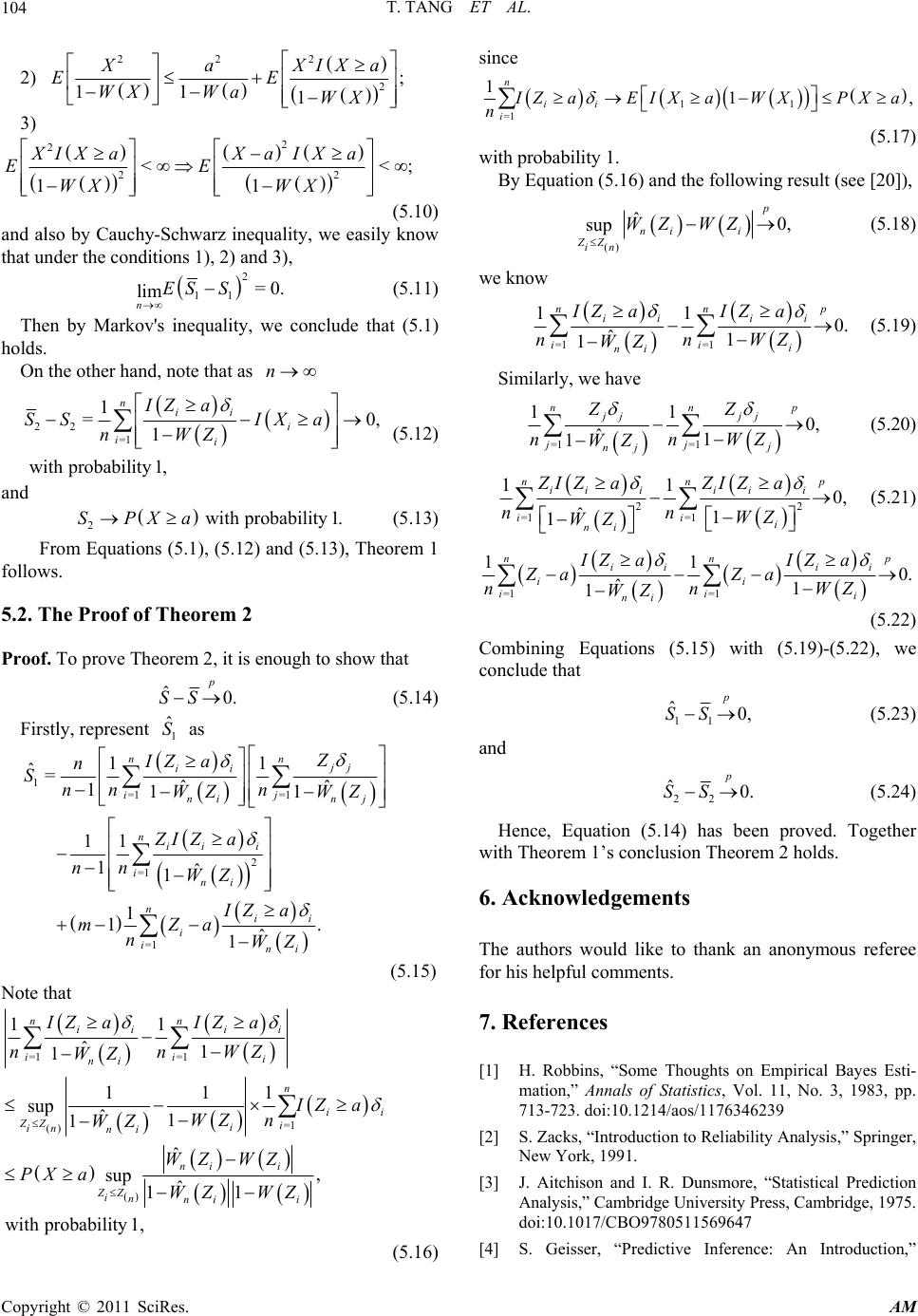

 







T. TANG ET AL. 104
2)
 



222
2;
11 1
XaXIXa
EE
WX WaWX

 




   
3)






2
2
22
<<;
11
XIXaX a IXa
EE
WX WX
 

 
 
 

(5.10)
and also by Cauchy-Schwarz inequality, we easily know
that under the conditions 1), 2) and 3),

2
11
=0.
lim
nES S   (5.11)
Then by Markov's inequality, we conclude that (5.1)
holds.
On the other h a nd , not e that as n

 
22 =1
1
=0,
1
withprobability1,
niii
ii
IZ a
SS IXa
nWZ








 (5.12)
and

2with probability1.SPXa (5.13)
From Equations (5.1), (5.12) and (5.13), Theorem 1
follows.
5.2. The Proof of Theorem 2
Proof. To prove Theorem 2, it is enough to show that
ˆ0.
p
SS (5.14)
Firstly, represent 1
ˆ
S as




 




1=1 =1
2
=1
=1
11
ˆ=ˆˆ
111
11
1ˆ
1
1
1.
ˆ
1
nn
jj
ii
ij
ninj
nii i
ini
nii
i
ini
Z IZ a
n
Snn n
WZ WZ
ZI Za
nn WZ
IZ a
mZa
nWZ
 



















 



(5.15)
Note that




  


 
 
=1 =1
=1
()
11
ˆ1
1
111
sup ˆ1
1
ˆ,
sup ˆ
11
with probability1,
nn
ii ii
ii
i
ni
n
ii
ZZ i
i
in ni
ni i
ZZ
inni i
IZ aIZ a
nnWZ
WZ
IZ a
WZ n
WZ
WZ WZ
PX aWZWZ











 


(5.16)
since
  

11
=1
11,
n
ii
i
IZaEIXaWXPX a
n


 


(5.17)
with probability 1.
By Equation (5.16) and the following result (see [20]),
 
()
ˆ0,
sup p
ni i
ZZ
in
WZ WZ

 (5.18)
we know





=1 =1
11 0.
ˆ1
1
nn p
ii ii
ii
i
ni
IZ aIZ a
nnWZ
WZ
 



 (5.19)
Similarly, we have
 
=1 =1
110,
ˆ1
1
nn p
jj jj
jj
j
nj
ZZ
nnWZ
WZ




 (5.20)





22
=1 =1
11 0,
ˆ1
1
nn p
ii iii i
ii
i
ni
ZI ZaZI Za
nn
WZ
WZ
 

 


 (5.21)



 



=1 =1
11 0.
ˆ1
1
nn p
ii ii
ii
ii
i
ni
IZ aIZ a
Za Za
nnWZ
WZ
 




(5.22)
Combining Equations (5.15) with (5.19)-(5.22), we
conclude that
11
ˆ0,
p
SS (5.23)
and
22
ˆ0.
p
SS

 (5.24)
Hence, Equation (5.14) has been proved. Together
with Theorem 1’s conclusion Theorem 2 holds.
6. Acknowledgements
The authors would like to thank an anonymous referee
for his helpful comments.
7. References
[1] H. Robbins, “Some Thoughts on Empirical Bayes Esti-
mation,” Annals of Statistics, Vol. 11, No. 3, 1983, pp.
713-723. doi:10.1214/aos/1176346239
[2] S. Zacks, “Introduction to Reliability Analysis,” Springer,
New York, 1991.
[3] J. Aitchison and I. R. Dunsmore, “Statistical Prediction
Analysis,” Cambridge University Press, Cambridge, 1975.
doi:10.1017/CBO9780511569647
[4] S. Geisser, “Predictive Inference: An Introduction,”

T. TANG ET AL. 105
Chapman and Hall, London, 1993.
[5] L. J. Bain and M. Engelhardt, “Interval Estimation for the
Two-Parameter Double Exponential Distribution,” Tech-
nometrics, Vol. 15, No. 4, 1973, pp. 875-887. doi:
10.2307/1267397
[6] R. G. Easterling, “Exponential Responses with Double
Exponetial Distribution Measurement Error-A Model for
Steam Generator Inspection,” Proceedings of the DOE
Statistical Symposium, U.S. Department of Energy, 1978,
pp. 90-110.
[7] M. T. Madi and T. Leonard, “Bayesian Estimation for
Shifted Exponential Distribution,” Journal of Statistical
Planning and Inference, Vol. 55, No. 6, 1996, pp.
345-351. doi:10.1016/S0378-3758(95)00199-9
[8] W. T. Huang and H. H. Huang, “Empirical Bayes Esti-
mation of the Guarantee Lifetime in a Two-Parameter
Exponential Distribution,” Statistics and Probability Let-
ters, Vol. 76, No. 16, 2006, pp. 1821-1829. doi:10.1016/
j.spl.2006.04.034
[9] J. W. Wu, H. M. Lee and C. L. Lei, “Computational
Testing Algorithmic Procedure of Assessment for Life-
time Performance Index of Products with Two-Parameter
Exponential Distribution,” Applied Mathematics and
Computation, Vol. 190, No. 5, 2007, pp. 116-125. doi:
10.1016/j.amc.2007.01.010
[10] J. O. Berger, “Statistical Decision Theory and Bayesian
Analysis,” Springer, New York, 1985.
[11] R. S. Singh, “Bayes and Empirical Bayes Procedures for
Selecting Good Populations from a Translated Exponen-
tial Family,” Empirical Bayes and Likelihood Inference,
Springer, New York, 2001.
[12] H. Lian, “Consistency of Bayesian Estimation of a Step
Function,” Statistics and Probability Letters, Vol. 77, No.
1, 2007, pp. 19-24. doi:10.1016/j.spl.2006.05.007
[13] Q. H. Wang, “Empirical Likelihood for a Class of Func-
tions of Survival Distribution with Censored Data,” An-
nals of the Institute of Statistical Mathematics, Vol. 53,
No. 3, 2001, pp. 517-527. doi:10.1023/A:1014617112870
[14] E. T. Kaplan and P. Meier, “Nonparametric Estimation
from Incomplete Observations,” Journal of the American
Statistical Association, Vol. 53, No. 282, 1958, pp. 457-
481. doi:10.2307/2281868
[15] R. Y. Zheng, “Improvement on Grey Modelling Ap-
proach and Its Applications to Fatigue Reliability Re-
search,” Master Dissertation, National University of De-
fense Technology, Chang Sha, 1989.
[16] K. O. Bowman and L. R. Shenton, “Weibull Distributions
When the Shape Parameter is Defined,” Computational
Statistics and Data Analysis, Vol. 36, No. 4, 2001, pp.
299-310. doi:10.1016/S0167-9473(00)00048-7
[17] U. Singh, P. K. Gupta and S. K. Upadhyay, “Estimation
of Parameters for Exponentiated-Weibull Family Under
Type-II Censoring Scheme,” Computational Statistics
and Data Analysis, Vol. 48, No. 3, 2005, pp. 509-523.
doi:10.1016/j.csda.2004.02.009
[18] L. F. Zhang, M. Xie and L. C. Tang, “A Study of Two
Estimation Approaches for Parameters of Weibull Dis-
tribution Based on WPP,” Reliability Engineering and
System Safety, Vol. 92, No. 3, 2007, pp. 360-368. doi:
10.1016/j.ress.2006.04.008
[19] Z. F. Jaheen, “Bayesian Prediction Under a Mixture of
Two-Component Gompertz Lifetime Model,” Test, Vol.
12, No. 1, 2003, pp. 413-426. doi:10.1007/BF02595722
[20] M. Zhou, “Asymptotic Normality of the Synthetic Data
Regression Estimation for Censored Survival Data,” An-
nals of Statistics, Vol. 20, No. 2, 1992, pp. 1002-1021.
doi:10.1214/aos/1176348667.