Paper Menu >>
Journal Menu >>
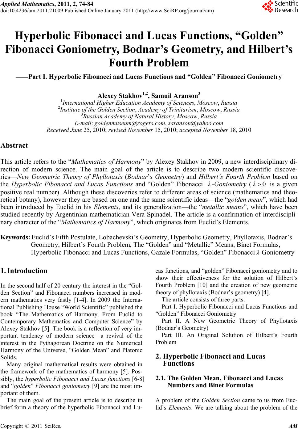 Applied Mathematics, 2011, 2, 74-84 doi:10.4236/am.2011.21009 Published Online January 2011 (http://www.SciRP.org/journal/am) Copyright © 2011 SciRes. AM Hyperbolic Fibonacci and Lucas Functions, “Golden” Fibonacci Goniometry, Bodnar’s Geometry, and Hilbert’s Fourth Problem ——Part I. Hyperbolic Fibonacci and Lucas Functions and “Golden” Fibonacci Goniometry Alexey Stakhov1,2, Samuil Aranson3 1International Higher Education Academy of Sciences, Moscow, Russia 2Institute of the Golden Section, Academy of Trinitarism, Moscow, Russia 3Russian Academy of Natural History, Moscow, Russia E-mail: goldenmuseum@rogers.com, saranson@yahoo.com Received June 25, 2010; revised November 15, 2010; accepted November 18, 2010 Abstract This article refers to the “Mathematics of Harmony” by Alexey Stakhov in 2009, a new interdisciplinary di- rection of modern science. The main goal of the article is to describe two modern scientific discove- ries—New Geometric Theory of Phyllotaxis (Bodnar’s Geometry) and Hilbert’s Fourth Problem based on the Hyperbolic Fibonacci and Lucas Functions and “Golden” Fibonacci λ-Goniometry (λ is a given positive real number). Although these discoveries refer to different areas of science (mathematics and theo- retical botany), however they are based on one and the same scientific ideas—the “golden mean”, which had been introduced by Euclid in his Elements, and its generalization—the “metallic means”, which have been studied recently by Argentinian mathematician Vera Spinadel. The article is a confirmation of interdiscipli- nary character of the “Mathematics of Harmony”, which originates from Euclid’s Elements. Keywords: Euclid’s Fifth Postulate, Lobachevski’s Geometry, Hyperbolic Geometry, Phyllotaxis, Bodnar’s Geometry, Hilbert’s Fourth Problem, The “Golden” and “Metallic” Means, Binet Formulas, Hyperbolic Fibonacci and Lucas Functions, Gazale Formulas, “Golden” Fibonacci λ-Goniometry 1. Introduction In the second half of 20 century the interest in the “Gol- den Section” and Fibonacci numbers increased in mod- ern mathematics very fastly [1-4]. In 2009 the Interna- tional Publishing House “World Scientific” published the book “The Mathematics of Harmony. From Euclid to Contemporary Mathematics and Computer Science” by Alexey Stakhov [5]. The book is a reflection of very im- portant tendency of modern science—a revival of the interest in the Pythagorean Doctrine on the Numerical Harmony of the Universe, “Golden Mean” and Platonic Solids. Many original mathematical results were obtained in the framework of the mathematics of harmony [5]. Pos- sibly, the hyperbolic Fibonacci and Lucas functions [6-8] and “golden” Fibonacci goniometry [9] are the most im- portant of them. The main goal of the present article is to describe in brief form a theory of the hyperbolic Fibonacci and Lu- cas functions, and “golden” Fibonacci goniometry and to show their effectiveness for the solution of Hilbert’s Fourth Problem [10] and the creation of new geometric theory of phyllotaxis (Bodnar’s geometry) [4]. The article consists of three parts: Part I. Hyperbolic Fibonacci and Lucas Functions and “Golden” Fibonacci Goniometry Part II. A New Geometric Theory of Phyllotaxis (Bodnar’s Geom et ry) Part III. An Original Solution of Hilbert’s Fourth Problem 2. Hyperbolic Fibonacci and Lucas Functions 2.1. The Golden Mean, Fibonacci and Lucas Numbers and Binet Formulas A problem of the Golden Section came to us from Euc- lid’s Elements. We are talking about the problem of the 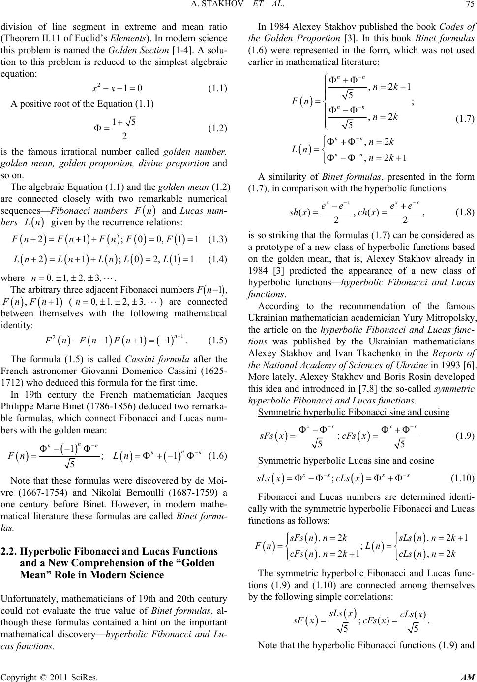 A. STAKHOV ET AL. Copyright © 2011 SciRes. AM 75 division of line segment in extreme and mean ratio (Theorem II.11 of Euclid’s Elements). In modern science this problem is named the Golden Section [1-4]. A solu- tion to this problem is reduced to the simplest algebraic equation: 210xx (1.1) A positive root of the Equ a tion (1.1) 15 2 (1.2) is the famous irrational number called golden number, golden mean, golden proportion, divine proportion and so on. The algebraic Equation (1.1) and the golden mean (1.2) are connected closely with two remarkable numerical sequences—Fibonacci numbers F n and Lucas num- bers Ln given by the recurrence relations: 21;00,11FnFnFn FF (1.3) 21;02,11LnLnLn LL (1.4) where 0,1,2,3,n. The arbitrary three adjacent Fibonacci nu mbers 1,Fn ,1Fn Fn (0, 1,2,3,n) are connected between themselves with the following mathematical identity: 1 2111. n Fn FnFn (1.5) The formula (1.5) is called Cassini formula after the French astronomer Giovanni Domenico Cassini (1625- 1712) who deduced this formula for the first time. In 19th century the French mathematician Jacques Philippe Marie Bine t (1786-1856) deduced two r emarka- ble formulas, which connect Fibonacci and Lucas num- bers with the golden mean: 1;1 5 n nn n nn Fn Ln (1.6) Note that these formulas were discovered by de Moi- vre (1667-1754) and Nikolai Bernoulli (1687-1759) a one century before Binet. However, in modern mathe- matical literature these formulas are called Binet formu- las. 2.2. Hyperbolic Fibonacci and Lucas Functions and a New Comprehension of the “Golden Mean” Role in Modern Science Unfortunately, mathematicians of 19th and 20th century could not evaluate the true value of Binet formulas, al- though these formulas contained a hint on the important mathematical discovery—hyperbolic Fibonacci and Lu- cas functions. In 1984 Alexey Stakhov published the book Codes of the Golden Proportion [3]. In this book Binet formulas (1.6) were represented in the form, which was not used earlier in mathematical literature: ,21 5; ,2 5 ,2 ,21 nn nn nn nn nk Fn nk nk Ln nk (1.7) A similarity of Binet formulas, presented in the form (1.7), in comparison with the hyperbolic functions (), (), 22 x xxx ee ee sh xch x (1.8) is so striking that the formulas (1.7) can be considered as a prototype of a new class of hyperbolic functions based on the golden mean, that is, Alexey Stakhov already in 1984 [3] predicted the appearance of a new class of hyperbolic functions—hyperbolic Fibonacci and Lucas functions. According to the recommendation of the famous Ukrainian mathematician academician Yury Mitropolsky, the article on the hyperbolic Fibonacci and Lucas func- tions was published by the Ukrainian mathematicians Alexey Stakhov and Ivan Tkachenko in the Reports of the National Academy of Sciences of Ukraine in 1993 [6]. More lately, Alexey Stakhov and Boris Rosin developed this idea and introduced in [7,8] the so-called symmetric hyperbolic Fibonacci and Lucas functions. USymmetric hyperbolic Fibonacci sine and cosine ; 55 x xxx sFsx cFsx (1.9) USymmetric hyperbolic Lucas sine and cosine ; x xxx sLs xcLs x (1.10) Fibonacci and Lucas numbers are determined identi- cally with the symmetric hyperbolic Fibonacci and Lucas functions as follows: ,2 ,21 ; ,21 ,2 s Fs nnksLs nnk Fn Ln cFs nnkcLsnnk The symmetric hyperbolic Fibonacci and Lucas func- tions (1.9) and (1.10) are connected among themselves by the following simple correlations: () ;() . 55 sLs xcLs x sFxcFs x Note that the hyperbolic Fibonacci functions (1.9) and 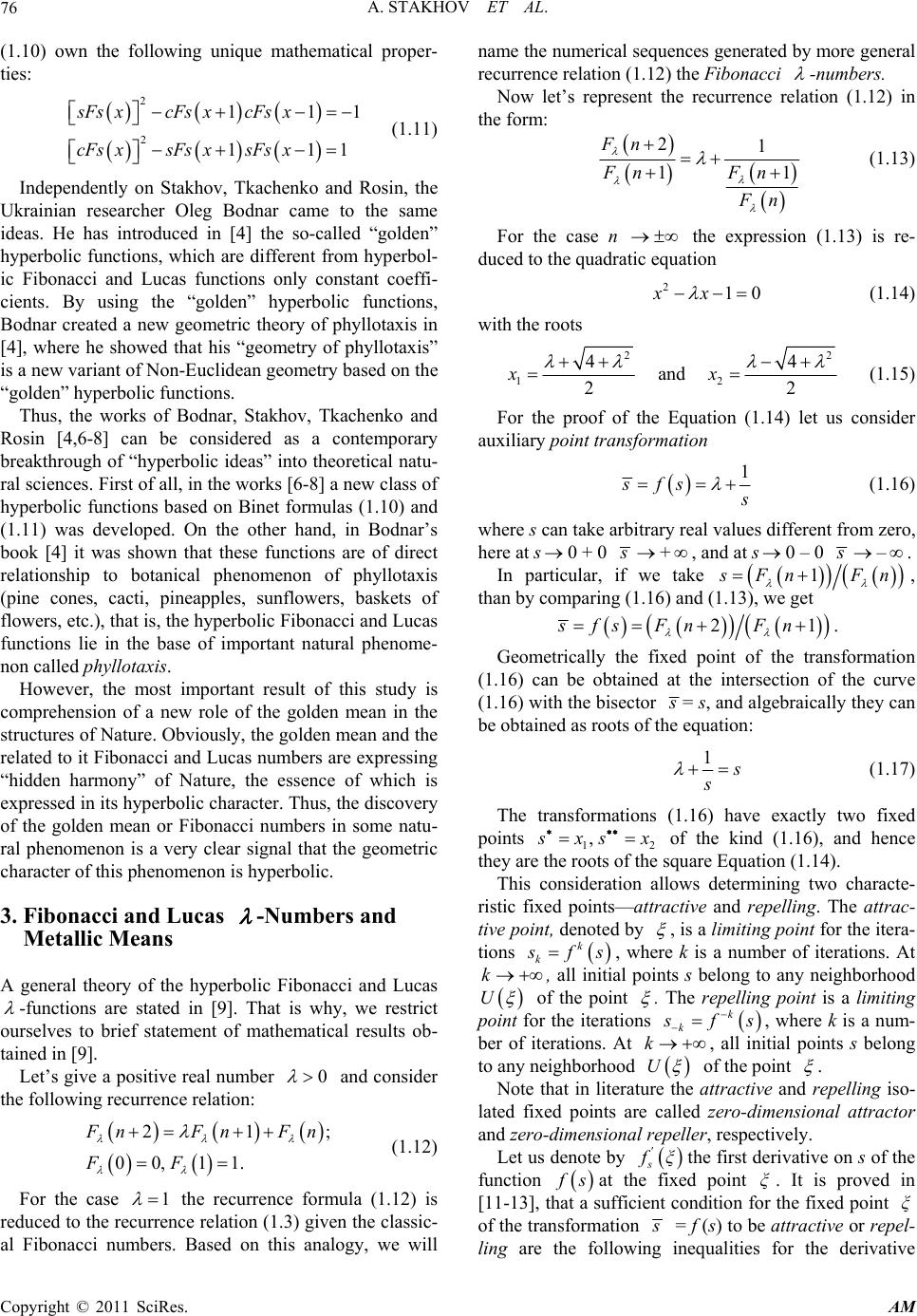 A. STAKHOV ET AL. Copyright © 2011 SciRes. AM 76 (1.10) own the following unique mathematical proper- ties: 2 2 111 111 sFsxcFsx cFsx cFsxsFsx sFsx (1.11) Independently on Stakhov, Tkachenko and Rosin, the Ukrainian researcher Oleg Bodnar came to the same ideas. He has introduced in [4] the so-called “golden” hyperbolic functions, which are different from hyperbol- ic Fibonacci and Lucas functions only constant coeffi- cients. By using the “golden” hyperbolic functions, Bodnar created a new geometric theory of phyllotaxis in [4], where he showed that his “geometry of phyllotaxis” is a new variant of Non-Euclidean geometry based on the “golden” hyperbolic functions. Thus, the works of Bodnar, Stakhov, Tkachenko and Rosin [4,6-8] can be considered as a contemporary breakthrough of “hyperbolic ideas” into theoretical natu- ral sciences. First of all, in the works [6-8] a new class of hyperbolic functions based on Binet formulas (1.10) and (1.11) was developed. On the other hand, in Bodnar’s book [4] it was shown that these functions are of direct relationship to botanical phenomenon of phyllotaxis (pine cones, cacti, pineapples, sunflowers, baskets of flowers, etc.), that is, the hyperbolic Fibonacci and Lucas functions lie in the base of important natural phenome- non called phyllotaxis. However, the most important result of this study is comprehension of a new role of the golden mean in the structures of Nature. Obviously, the golden mean and the related to it Fibonacci and Lucas numbers are expressing “hidden harmony” of Nature, the essence of which is expressed in its hyperbolic character. Thus, the discovery of the golden mean or Fibonacci numbers in some natu- ral phenomenon is a very clear signal that the geometric character of this phenomenon is hyperbolic. 3. Fibonacci and Lucas -Numbers and Metallic Means A general theory of the hyperbolic Fibonacci and Lucas -functions are stated in [9]. That is why, we restrict ourselves to brief statement of mathematical results ob- tained in [9]. Let’s give a positive real number 0 and consider the following recurrence relation: 21; 00, 11. F nFnFn FF (1.12) For the case 1 the recurrence formula (1.12) is reduced to the recurrence relation (1.3) given the classic- al Fibonacci numbers. Based on this analogy, we will name the numerical sequences generated by more general recurrence rela tion (1 . 1 2) the Fibonacci -numbers. Now let’s represent the recurrence relation (1.12) in the form: 21 1 1 Fn Fn Fn F n (1.13) For the case n the expression (1.13) is re- duced to the quadratic equation 210xx (1.14) with the roots 2 14 2 x and 2 24 2 x (1.15) For the proof of the Equation (1.14) let us consider auxiliary point transformation 1 sfs s (1.16) where s can take arbitrary real values different from zero, here at s0 + 0 s + , and at s0 – 0 s – . In particular, if we take 1 s Fn Fn , than by comparing (1.16) and (1.13), we get 21sfs FnFn . Geometrically the fixed point of the transformation (1.16) can be obtained at the intersection of the curve (1.16) with the bisector s = s, and algebraically they can be obtained as roots of the equation: 1 s s (1.17) The transformations (1.16) have exactly two fixed points 12 , s xs x of the kind (1.16), and hence they are the roots of the square Equation (1.14). This consideration allows determining two characte- ristic fixed points—attractive and repelling. The attrac- tive point, denoted by , is a limiting point for the itera- tions k k s fs, where k is a number of iterations. At k, all initial points s belong to any neighborhood U of the point . The repelling point is a limiting point for the iterations k k s fs , where k is a num- ber of iterations. At k, all initial points s belong to any neighborhood U of the point . Note that in literature the attractive and repelling iso- lated fixed points are called zero-dimensional attractor and zero-dimensional repeller, respectively. Let us denote by s fξ the first derivative on s of the function f sat the fixed point ξ. It is proved in [11-13], that a sufficient condition for the fixed point ξ of the transformation s = f (s) to be attractive or repel- ling are the following inequalities for the derivative 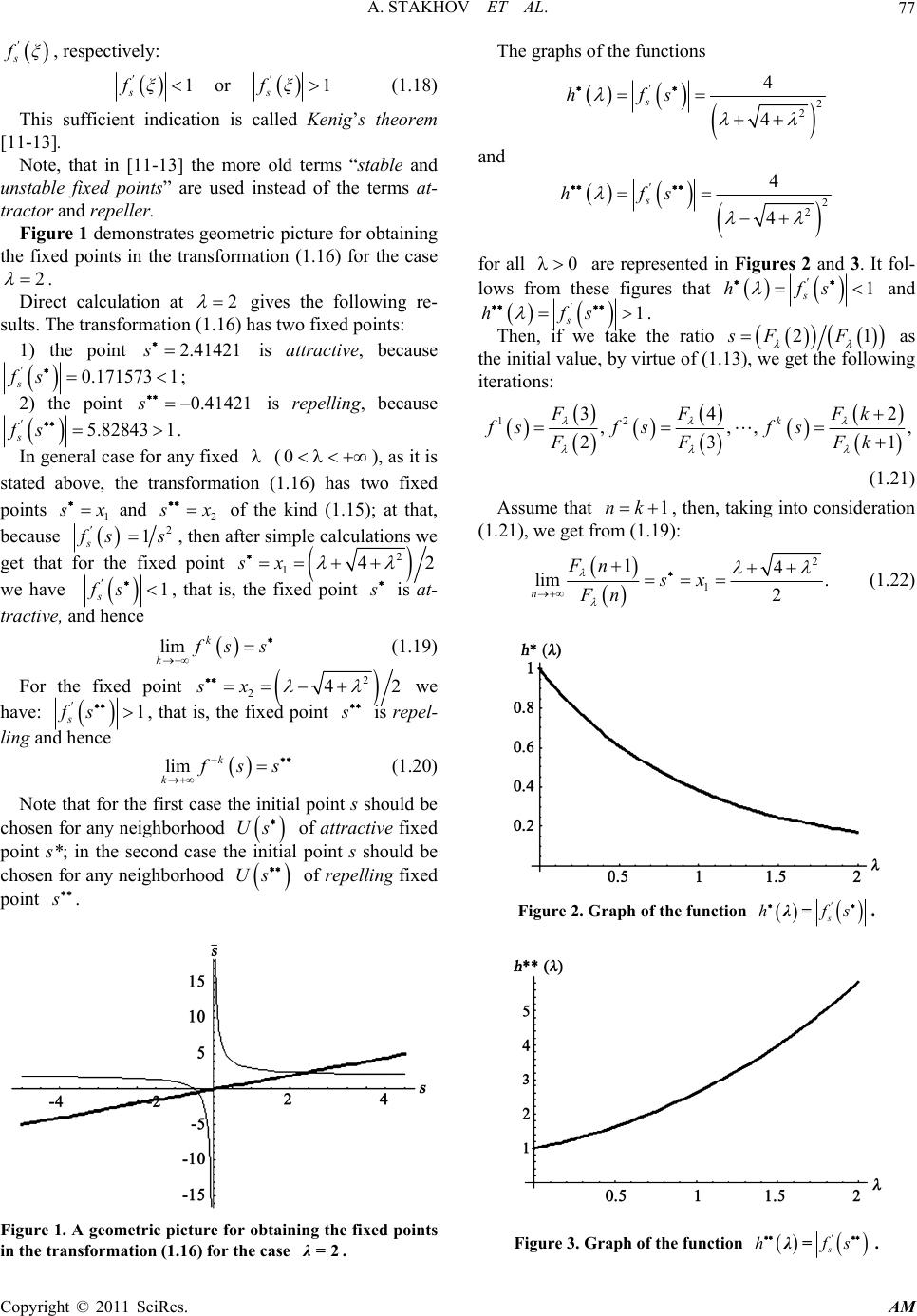 A. STAKHOV ET AL. Copyright © 2011 SciRes. AM 77 s fξ , respectively: 1 s fξ or 1 s fξ (1.18) This sufficient indication is called Kenig’s theorem [11-13]. Note, that in [11-13] the more old terms “stable and unstable fixed points” are used instead of the terms at- tractor and repeller. Figure 1 demonstrates geometric picture for obtaining the fixed points in the transformation (1.16) for the case 2 . Direct calculation at 2 gives the following re- sults. The transformation (1.16) has two fixed points: 1) the point 2.41421s is attractive, because 0.171573 1 s fs ; 2) the point 0.41421s is repelling, because 5.82843 1 s fs . In general case for any fixed (0 ), as it is stated above, the transformation (1.16) has two fixed points 1 s x and 2 s x of the kind (1.15); at that, because 2 1 s f ss , then after simple calculations we get that for the fixed point 2 142sx we have 1 s fs , that is, the fixed point s is at- tractive, and hence lim k k f ss (1.19) For the fixed point 2 242sx we have: 1 s fs , that is, the fixed point s is repel- ling and hence lim k k f ss (1.20) Note that for the first case the initial point s should be chosen for any neighborho od Us of attractive fixed point s*; in the second case the initial point s should be chosen for any neighborh ood Us of repelling fixed point s . Figure 1. A geometric picture for obtaining the fixed points in the transformation (1.16) for the case =2λ. The graphs of the functions 2 2 4 4 s hfs and 2 2 4 4 s hfs for all 0 are represented in Figures 2 and 3. It fol- lows from these figures that 1 s hfs and 1 s hfs . Then, if we take the ratio 21sF F as the initial value, by virtue of (1.13), we get the following iterations: 12 34 2 ,,, , 23 1 k FF Fk fsf sf s FF Fk (1.21) Assume that 1nk , then, taking into consideration (1.21), we get from (1.1 9): 2 1 14 lim . 2 n Fn sx Fn (1.22) Figure 2. Graph of the function s hfs = λ. Figure 3. Graph of the function s hfs = λ.  A. STAKHOV ET AL. Copyright © 2011 SciRes. AM 78 By analogy, if we take into consideration (1.21), we get: 2 24 lim . 12 n Fn sx Fn (1.23) Let us denote a positive root x1 by and consider a new class of mathematical constants given by the fol- lowing formula: 2 4. 2 (1.24) Note that for the case 1 the formula (1.24) takes the form (1.2) given the classical golden mean. The Argentinean mathematician Vera W. Spin adel [14] named the mathematical constants generated by (1.24) metallic means. If we take =1, 2, 3, 4 in (1.24), then we get the following mathematical constants having ac- cording to Vera Spinadel special names: 1 2 3 4 15 the Golden Mean,1; 2 12the Silver Mean ,2; 313 the Bronze Mean,3; 2 25the Cooper Mean,4. Other metallic means (5 ) do not have special names: 56 78 529 ;3210; 2 7214 ;417. 2 It is easy to prove that the root x2 can be represented by the metallic mean (1.24) as follows: 2 214 . 2 x (1.25) By using the algebraic Equation (1.14), it is easy to prove the following remarkable algebraic properties of the metallic means (1.24): 1 111 ;11 (1.26) They are a generalization of the following mathemati- cal properties of the golden mean (1 ): 1 111 ;11 4. Gazale Formulas for the Fibonacci and Lucas -Numbers Based on the metallic means (1.24), Midchat Gazale in [15] has deduced remarkable formula, which gives Fi- bonacci -numbers (1.12) in analytical form: 2 1 4 n nn Fn (1.27) where n = 0, 1, 2, 3, ··· Alexey Stakhov in [9] has deduced the similar analyt- ical formula for the Lucas -numbers: 1, n nn Ln (1.28) where n = 0, 1, 2, 3, ··· The formulas (1.27) and (1.28) are named in [9] Ga- zale formulas after Midchat Gazale, who first has de- duced the formula (1.27) in the book [15]. Note that for the case 1 Gazale formulas (1.27) and (1.28) are reduced to the Binet formulas (1.6). As is shown in [9], the Lucas -numbers (1.28) can be given recursively in the form 12;02,11.Ln LnLnLL (1.29) Note that for the case 1 the Lucas -numbers, given by the recurrence relation (1.29), are reduced to the classical Lucas numbers. Now let us represent the Gazale formulas (1.27) and (1.28) for the negative values of n as follows: 2 1 4 n nn Fn (1.30) 1n nn Ln (1.31) Comparing the formulas (1.27) and (1.30) for the even (n = 2k) and odd (n = 2k + 1) values of n, we can con- clude that 22 F kFk and 21 21.FkF k (1.32) This means that for the given positive real number 0 the sequence of the Fibonacci -numbers ( 1.12) in the infinite range n=0, 1, 2, 3, ··· is a symmetrical sequence relatively to the Fibonacci -number 00F except that the Fibonacci -numbers 2 F k and 2 F k are opposite by sign. In Tabl e 1 we can see the Fibonacci -numbers F n for the cases 1,2, 3,4 . Note that for the case 2 the Gazale formula (1.27) generates a numerical sequence known as Pell numbers.  A. STAKHOV ET AL. Copyright © 2011 SciRes. AM 79 Table 1. The Fibonacci -sequences λ F n for the cases =1,2,3,4λ. n -5 -4 -3 -2 -1 0 1 2 3 4 5 1 5 -3 2 -1 1 0 1 1 2 3 5 2 29 -12 5 -2 1 0 1 2 5 12 29 3 109 -33 10 -3 1 0 1 3 10 33 109 4 305 -72 17 -4 1 0 1 4 17 72 305 Table 2. The Lucas -sequences λ Ln for the cases =1,2,3,4λ. n -5 -4 -3 -2 -1 0 1 2 3 4 5 1 -11 7 -4 3 -1 2 1 3 4 7 11 2 -82 34 -14 6 -2 2 2 6 14 34 82 3 -393 119 -36 11 -3 2 3 11 36 119 393 4 -1364 322 -76 18 -4 2 4 18 76 322 1364 Comparing the formulas (1.28) and (1.31) for the even (n = 2k) and odd (n = 2k + 1) values of n, we can con- clude that 22LkL k and 21 21LkL k (1.33) This means that for the given positive real number 0 the sequence of the Lucas -numbers in the range n=0, 1, 2, 3, ··· is a symmetrical sequence rela- tive to the Lucas -number 02L except that the Lucas numbers 21Lk and 21Lk are op- posite by sign. In Table 2 we can see the Lucas -numbers Ln for the cases . Note that for the case 2 the Gazale formula (1.28) generates the numerical sequence known as Pell-Lucas numbers. It is easy to deduce the following identity for the Fi- bonacci -numbers similar to the Cassini formula (1.5): 1 2111 n Fn FnFn (1.34) 5. “Golden” Fibonacci -Goniometry 5.1. A Definition of the Hyperbolic Fibonacci and Lucas -Functions First of all, let us explain the term of goniometry used in this article. As is known, a goniometry is a part of geo- metry, which sets relations between trigonometric func- tions. In this article we use instead of trigonometric func- tions the so-called symmetric hyperbolic Fibonacci and Lucas -functions introduced in [9]. Let us consider these functions. UHyperbolic Fibonacci U U-sine and U U-cosine 2 22 2 4 14 4 22 4 xx x x sF x (1.35) 2 22 2 4 14 4 22 4 xx x x cF x (1.36) UHyperbolic Lucas U U-sine and U U-cosine 22 44 22 xx x x sL x (1.37) 22 44 22 xx x x cL x (1.38) where x is continuous variable and is a given positive real number. The Fibonacci and Lucas -numbers are determined identically by the hyperbolic Fibonacci and Lucas -functions as follows:  A. STAKHOV ET AL. Copyright © 2011 SciRes. AM 80 (), 2 () ; (), 21 (), 2 () . (), 21 sF nnk Fn cF nnk cL nnk Ln sL nnk (1.39) It is easy to see that the functions (1.35)-(1.38) are connected by very simple correlations: 22 ;. 44 s Lx cLx sF xcF x (1.40) This means that the hyperbolic Lucas -functions (1.37) and (1.38) coincide with the hyperbolic Fibonacci -functions (1.35) and (1.36) to within of the constant coefficient 2 14 . Note that for the case 1 the hyperbolic Fibonacci and Lucas -functions (1.35)-(1.38) are reduced to the symmetric hyperbolic Fibonacci and Lucas functions (1.9) and (1.10). 5.2. Graphs of the Hyperbolic Fibonacci and Lucas -Functions The graphs of the hyperbolic Fibonacci and Lucas - functions are similar to the graphs of the symmetric hyperbolic Fibonacci and Lucas functions [7] (see Fig- ure 4). It is necessity to note that in the point x = 0, the hy- perbolic Fibonacci -cosine cF x (36) takes the value 2 024cF , and the hyperbolic Lucas cosine cL x (38) takes the value 02cL . It is also important to note that the Fibonacci λ -numbers F n with the even values of n = 0, 2, 4, 6, ··· are “inscribed” into the graph of the hyperbolic Fibonacci -sine s Fx in the discrete points x = 0, 2, 4, 6, ··· and the Fibonacci -numbers F n with the odd values of n = 1, 3, 5, ··· are “inscribed” into the hyperbolic Fibonacci -cosine cF x in the discrete points x = 1, 3, 5 ···. On the other hand, the Lucas -numbers Ln with the even values of n are “inscribed” into the graph of the hyperbolic Lucas -cosine cL x in the discrete points x = 0, 2, 4, 6 ···, and the Lucas -numbers Ln with the odd values of n are “inscribed” into the graph of the hyperbolic Lucas -sine s Lx in the discrete points x = 1, 3, 5 ···. By analogy with the symmetric hyperbolic Fibonacci and Lucas functions [7], we can introduce other kinds of the hyperbolic Fibonacci and Lucas -functions, in particular, hyperbolic Fibonacci and Lucas -tangents and -cotangents, -secants and -cosecants and so on. (a) (b) Figure 4. A graph of the symmetric hyperbolic Fibonacci functions (a) and Lucas functions (b). 5.3. Partial Cases of the Hyperbolic Fibonacci and Lucas -Functions The formulas (1.35)-(1.38) set an infinite number of the different hyperbolic -functions because every real number generates its own variant of the hyper- bolic Fibonacci and Lucas -functions of the kind (1.35)-(1.38). Let us consider the partial cases of the hyperbolic Fi- bonacci and Lucas -functions (1.35)-(1.38) for the different values of . For the case the “golden mean” (1.2) is a base of the hyperbolic Fibonacci and Lucas 1-functions, which are reduced to the symmetric hyperbolic Fibonacci and Lucas functions (1.9) and (1.10). Therefore in further we will name the functions (1.9) and (1.10) the “golden” hyperbolic Fibonacci and Lucas functions. For the case the “silver mean” 212 is a base of new class of hyperbolic functions. We will name them the “silver” hyperbolic Fibonacci and Lucas functions: 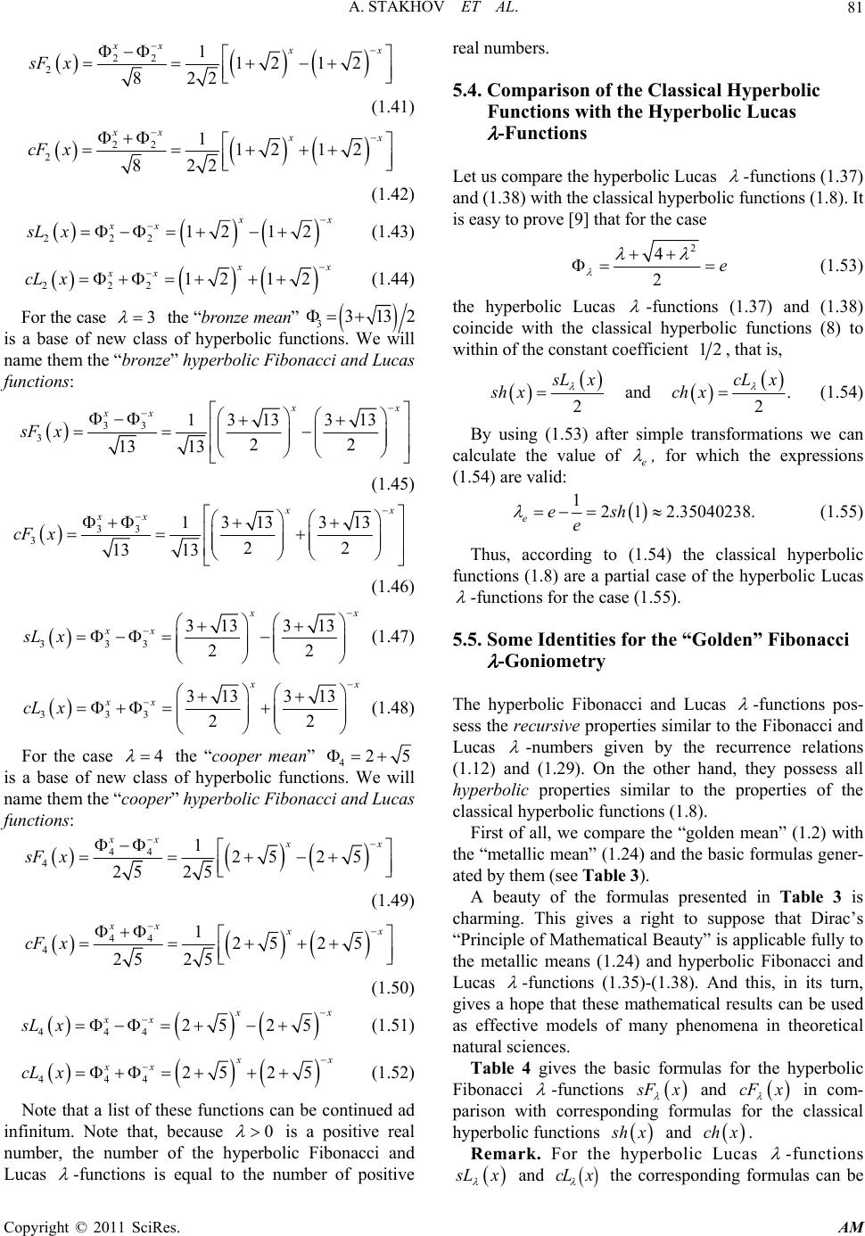 A. STAKHOV ET AL. Copyright © 2011 SciRes. AM 81 22 2112 12 822 xx x x sFx (1.41) 22 2112 12 822 xx x x cF x (1.42) 222 1212 x x xx sL x (1.43) 222 12 12 x x xx cL x (1.44) For the case the “bronze mean” 3313 2 is a base of new class of hyperbolic functions. We will name them the “bronze” hyperbolic Fibonacci and Lucas functions: 33 31313 313 22 13 13 x x xx sF x (1.45) 33 31313 313 22 13 13 x x xx cF x (1.46) 333 313 313 22 x x xx sL x (1.47) 333 313 313 22 x x xx cL x (1.48) For the case the “cooper mean” 425 is a base of new class of hyperbolic functions. We will name them the “cooper” hyperbolic Fibonacci and Lucas functions: 44 4125 25 25 25 xx x x sF x (1.49) 44 412525 25 25 xx x x cF x (1.50) 444 25 25 x x xx sL x (1.51) 444 25 25 x x xx cL x (1.52) Note that a list of these functions can be continued ad infinitum. Note that, because 0 is a positive real number, the number of the hyperbolic Fibonacci and Lucas -functions is equal to the number of positive real numbers. 5.4. Comparison of the Classical Hyperbolic Functions with the Hyperbolic Lucas -Functions Let us compare the hyperbolic Lucas -functions (1 .3 7) and (1.38) with the classical hyperbolic functions (1.8). It is easy to prove [9] that for the case 2 4 2e (1.53) the hyperbolic Lucas -functions (1.37) and (1.38) coincide with the classical hyperbolic functions (8) to within of the constant coefficient 12, that is, 2 s Lx sh x and . 2 cL x ch x (1.54) By using (1.53) after simple transformations we can calculate the value of e , for which the expressions (1.54) are valid: 12 1 2.35040238. eesh e (1.55) Thus, according to (1.54) the classical hyperbolic functions (1.8) are a partial case of the hyperbolic Lucas -functions for the case (1.55). 5.5. Some Identities for the “Golden” Fibonacci -Goniometry The hyperbolic Fibonacci and Lucas -functions pos- sess the recursive properties similar to the Fibonacci and Lucas -numbers given by the recurrence relations (1.12) and (1.29). On the other hand, they possess all hyperbolic properties similar to the properties of the classical hyperbolic functions (1.8). First of all, we compare the “golden mean” (1.2) with the “metallic mean” (1.24) and the basic formulas gener- ated by them (see Table 3). A beauty of the formulas presented in Table 3 is charming. This gives a right to suppose that Dirac’s “Principle of Mathematical Beauty” is applicable fully to the metallic means (1.24) and hyperbolic Fibonacci and Lucas -functions (1.35)-(1.38). And this, in its turn, gives a hope that these mathematical results can be used as effective models of many phenomena in theoretical natural sciences. Table 4 gives the basic formulas for the hyperbolic Fibonacci -functions s Fx and cF x in com- parison with corresponding formulas for the classical hyperbolic functions s hx and ch x . Remark. For the hyperbolic Lucas -functions s Lx and cL x the corresponding formulas can be 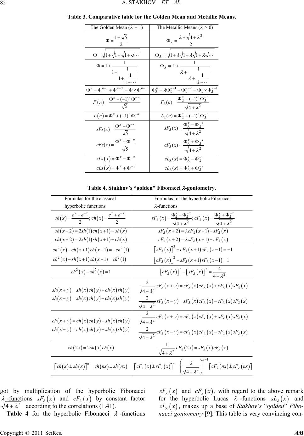 A. STAKHOV ET AL. Copyright © 2011 SciRes. AM 82 Table 3. Comparative table for the Golden Mean and Metallic Means. 2 12 1121 2 The Golden Mean ( = 1)The Metallic Means( > 0) 15 4 22 1111 1 1 11 111 111 11 (1) (1) () 54 nn nnnn nn nnn nnn FnF n Ln 2 2 (1)() (1) () () 54 () () 54 () () nnnnnn xx xx xx xx xx xx xx xx Ln sF x sFs x cFs xcF x sLs xsLx cLs xcLx Table 4. Stakhov’s “golden” Fibonacci -goniometry. 22 Formulas for the classical Formulas for the hy perbolic Fibonacci hyperbolic functions -functions ;; 22 44 221 1 221 1 xx xx xx xx ee ee sh xch xsFxcFx sh xshch xshxsFx ch xshshxchx 2 22 222 22 22 2 21 21 111 111 111 111 4 14 2 4 cF xsF x cF xsF xcF x sF xcF xcF x shxch xch xch chxsh xsh xchcF xsF xsF x ch xshxcF xsF x sh xysh xch ych xshy sh xysh xchychx sh y 2 2 2 2 2 2 4 2 4 2 4 1 22 2 4 n s FxysFxcFx cFxsFx s FxysFxcFx cFxsFx cF x ycFxcFxsF xsF x chxychxchyshxshy chxychxchyshxshycF xycFxcFxsF xsF x chxshx chxcFxsFx cFx chxshxch nx 1 2 2 4 n n s hnxcFx sFxcFnx sFnx got by multiplication of the hyperbolic Fibonacci -functions s Fx and cF x by constant factor 2 4 according to the correlations (1.41). Table 4 for the hyperbolic Fibonacci -functions s Fx and cF x , with regard to the above remark for the hyperbolic Lucas -functions s Lx and cL x , makes up a base of Stakhov’s “gold en” Fibo- nacci goniometry [9]. This table is very convincing con- 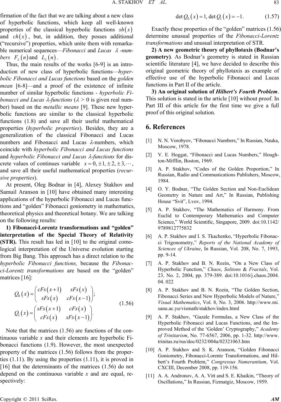 A. STAKHOV ET AL. Copyright © 2011 SciRes. AM 83 firmation of the fact that we are talking about a new class of hyperbolic functions, which keep all well-known properties of the classical hyperbolic functions s hx and ch x, but, in addition, they posses additional (“recursive”) properties, which unite them with remarka- ble numerical sequences—Fibonacci and Lucas -num- bers F n and Ln . Thus, the main results of the works [6-9] is an intro- duction of new class of hyperbolic functions—hyper- bolic Fibonacci and Lucas functions based on the golden mean [6-8]—and a proof of the existence of infinite number of similar hyperbolic functions - hyperbolic Fi- bonacci and Lucas -functions ( > 0 is given real num- ber) based on the metallic means [9]. These new hyper- bolic functions are similar to the classical hyperbolic functions (1.8) and save all their useful mathematical properties (hyperbolic properties). Besides, they are a generalization of the classical Fibonacci and Lucas numbers and Fibonacci and Lucas -numbers, which coincide with hyperbolic Fibonacci and Lucas functions and hyperbolic Fibonacci and Lucas -functions for dis- crete values of continues variable 0, 1,2,3,x, and save all their useful mathematical properties (recur- sive properties). At present, Oleg Bodnar in [4], Alexey Stakhov and Samuil Aranson in [10] have obtained many interesting applications of the hyperbolic Fibonacci and Lucas func- tions and “golden” Fibonacci goniometry in mathematics, theoretical physics and theoretical botany. We are talking on the following results: 1) Fibonacci-Lorentz transformations and “golden” interpretation of the Special Theory of Relativity (STR). This result has led in [10] to the original como- logical interpretation of the Universe evolution starting from Big Bang. This approach has a direct relation to the hyperbolic Fibonacci functions, because the Fibonac- ci-Lorentz transformations are based on the “golden” matrices [16]: 0 1. 1; 1 1 1 cFs xsFs x Qx sFsx cFsx sFsx cFsx Qx cFs xsFs x (1.56) Note that the matrices (1.56) are functions of the con- tinuous variable x and their elements are hyperbolic Fi- bonacci functions (1.9). However, the most unexpected property of the matrices (1.56) follows from the proper- ties (1.11). By using the properties (1.11), it is prov ed in [16] that the determinants of the matrices (1.56) do not depend on the continuous variable x and are equal, re- spectively: 01 det1, det1.Qx Qx (1.57) Exactly these properties of the “golden” matrices (1.56) determine unusual properties of the Fibonacci-Lorentz transformations and unus ual i nterpretation o f STR. 2) A new geometric theory of phyllotaxis (Bodnar’s geometry). As Bodnar’s geometry is stated in Russian scientific literature [4], we have decided to describe this original geometric theory of phyllotaxis as example of effective use of the hyperbolic Fibonacci and Lucas functions in Part II of the article. 3) An original solution of Hilbert’s Fourth Problem. This solution is stated in the article [10] without proof. In Part III of this article for the first time we give a full proof of this original solution. 6. References [1] N. N. Vorobyov, “Fibonacci Numbers,” In Russian, Nauka, Moscow, 1978. [2] V. E. Hoggat, “Fibonacci and Lucas Numbers,” Hough- ton-Mifflin, Boston, 1969. [3] A. P. Stakhov, “Codes of the Golden Proportion,” In Russian, Radio and Communications Publishers, Moscow, 1984. [4] O. Y. Bodnar, “The Golden Section and Non-Euclidean Geometry in Nature and Art,” In Russian, Publishing House “Svit”, Lvov, 1994. [5] A. P. Stakhov, “The Mathematics of Harmony. From Euclid to Contemporary Mathematics and Computer Science,” World Scientific, Singapore, 2009. doi:10.1142/ 9789812775832 [6] A. P. Stakhov and I. S. Tkachenko, “Hyperbolic Fibonac- ci Trigonometry,” Reports of the National Academy of Sciences of Ukraine, In Russian, Vol. 208, No. 7, 1993, pp. 9-14. [7] A. P. Stakhov and B. N. Rozin, “On a New Class of Hyperbolic Function,” Chaos, Solitons & Fractals, Vol. 23, No. 2, 2004, pp. 379-389. doi:10.1016/j.chaos.2004. 04. 022 [8] A. P. Stakhov and B. N. Rozin, “The Golden Section, Fibonacci Series and New Hyperbolic Models of Nature,” Visual Mathematics, Vol. 8, No. 3, 2006. http://www.mi. sanu.ac.yu/vismath/stakhov/index.html [9] A. P. Stakhov, “Gazale Formulas, a New Class of the Hyperbolic Fibonacci and Lucas Functions, and the Im- proved Method of the ‘Golden’ Cryptography,” Academy of Trinitarism, No. 77-6567, 2006, pp. 1-32. http://www. trinitas.ru/rus/doc/0232/004a/02321063.htm [10] A. P. Stakhov and S. K. Aranson, “Golden Fibonacci Goniometry, Fibonacci-Lorentz Transformations, and Hil- bert’s Fourth Problem,” Congressus Numerantium, Vol. CXCIII, December 2008, pp. 119-156. [11] A. A. Andronov, A. A. Vitt and S. E. Khaikin, “Theory of Oscillations,” In Russian, Fizmatgiz, Moscow, 1959.  A. STAKHOV ET AL. Copyright © 2011 SciRes. AM 84 [12] N. N. Bautin and E. A. Leontovich, “Methods and Ways of Qualitative Study of Dynamic Systems on a Plane,” In Russian, Nauka, Moscow, 1976. [13] J. I. Neimark, “Methods of Point Mappings in Theory of Non-Linear Oscillations,” In Russian, Nauka, Moscow, 1972. [14] V. W. de Spinadel, “From the Golden Mean to Chaos,” Nueva Libreria, Buenos Aires, 1998. [15] M. J. Gazale, “Gnomon. From Pharaohs to Fractals,” Princeton University Press, Princeton, 1999. [16] A. P. Stakhov, “The ‘Golden’ Matrices and a New Kind of Cryptography,” Chaos, Solitons & Fractals, Vol. 32, No. 3, 2007, pp. 1138-1146. doi:10.1016/j.chaos.2006. 03.069 |