Applied Mathematics, 2011, 2, 64-73
doi:10.4236/am.2011.21008 Published Online January 2011 (http://www.SciRP.org/journal/am)
Fuzzy Least-Squares Linear Regression Approach to
Ascertain Stochastic Demand in the Vehicle
Routing Problem
Fatemeh Torfi1,2, Reza Zanjirani Farahani3, Iraj Mahdavi1
1Department of Industrial Engineering, Islamic Azad University, Semnan Branch, Semnan, Iran
2Department of Industrial Engineering, Mazandaran University of Science and Technology, Babol, Iran
3Department of Industrial Engineering, Amirkabir University of Technology, Tehran, Iran
Received September 5, 2010; revised November 13, 2010; accepted November 17, 2010
Abstract
Estimation of stochastic demand in physical distribution in general and efficient transport routs management
in particular is emerging as a crucial factor in urban planning domain. It is particularly important in some
municipalities such as Tehran where a sound demand management calls for a realistic analysis of the routing
system. The methodology involved critically investigating a fuzzy least-squares linear regression approach
(FLLRs) to estimate the stochastic demands in the vehicle routing problem (VRP) bearing in mind the cus-
tomer's preferences order. A FLLR method is proposed in solving the VRP with stochastic demands: ap-
proximate-distance fuzzy least-squares (ADFL) estimator ADFL estimator is applied to original data taken
from a case study. The SSR values of the ADFL esti mator and real demand are obtained and then compared
to SSR values of the nominal demand and real demand. Empirical results showed that the proposed method
can be viable in solving problems under circumstances of having vague and imprecise performance ratings.
The results further proved that application of the ADFL was realistic and efficient estimator to face the sto-
chastic demand challenges in vehicle routing system management and solve relevant problems.
Keywords: Fuzzy Least-Squares, Stochastic, Location, Routing Problems
1. Introduction
The problem within distribution management of sched-
uling vehicles from one or more fixed positions (depots)
to service a given set of locations (customers) is called
the vehicle routing problem (VRP) [1]. Vehicle routing
problems are important and well-known combinatorial
optimization problems occurring in many transport logis-
tics and distribution systems of considerable economic
significance vehicle routing problem with stochastic de-
mand (VRPSD) has recently received a lot of attention in
the literature [2]. This is mainly because of the wide ap-
plicability of stochastic demand in real-world cases. In
the routing problem with stochastic demands (RPSD) a
vehicle has to serve a set of customers whose exact de-
mand is known on ly upon arrival at the customer’s loca-
tion. The objective in these problems is to find a permu-
tation of the customer's demands that the penalties for
losing a customer are minimized [3]. The actual demand
of each customer depends on common assumptions on
mathematical programming where all problem data are
known in advance. In most cases, however, decisions
have to be made before the realizations of random vari-
ables are known. A classical approach is to work with
estimations of random data and to solve the stochastic
problem similar to the deterministic cases. Moreover, it
is often preferable to explicitly incorpo rate uncertainty in
the models. Fuzzy Theory is a powerful tool, for decision
making in fuzzy environment. Crisp methods work only
with exact and ordinary data, so there is no place for
fuzzy and vagueness data. Torfi et al. [4] proposed a
Fuzzy approach to evaluate the alternative options in
respect to the user's preference orders in a fuzzy envi-
ronment. Human has a good ability for qualitative data
processing, which helps him or her to make decisions in
fuzzy environment. In many practical cases, decisions
are uncertain and they are reluctant or unable to make
numerical input and output data. Torfi et al. [5] applied a

F. TORFI ET AL. 65
new fuzzy decision making model to determine the wei-
ghts of multiple objectiv es in combinational op timization
problems.
In this paper, we apply their basic approximation op-
erations in fuzzy least-squares estimator. This paper con-
siders a stochastic routing problem in which a set of cus-
tomers is given, each of which will require service after
the a priori decision is made. Uncertainty is modeled by
using a vector of dependent variables which are interval-
lic and similar to the demand vector. Each of these in
turn depends on independent variables which are also
intervallic. However, in many practical cases, the cus-
tomer's demands are uncertain and those who demand
service are reluctant or unable to make a numerical per-
mutation of the customer's demands. Fuzzy least squares
linear regression was assumed to be a powerful tool for
decision-making in fuzzy environment. Fuzzy regression
analysis is a fuzzy (or possibility) type of classical re-
gression analysis. It is applied under circumstances
where evaluation of the functional relationship between
the dependent and independent variables in a fuzzy en-
vironment is necessary.
Tanaka et al. [6] initiated a study in fuzzy linear re-
gression analysis that considered the parameter estima-
tion of models as linear programming problems. Based
on the findings of Tanaka et al., further investigations
were made, which took two approaches: the linear-pro-
gramming-based methods [6-9] and fuzzy least-squares
methods [10-12]. Most of these fuzzy regression models
are analytically considered with fuzzy outputs and fuzzy
parameters but non-fuzzy (crisp) inputs. This paper aims
to study fuzzy linear regression model with fuzzy outputs,
fuzzy parameters, and fuzzy i nputs.
Sakawa and Yano [9] proposed a fuzzy parameter es-
timation model for the fuzzy linear regression (FLR)
model as follows:
011 , 1,2,,. ijkjk
YAAX AXjn 
Where both input data Xj1, Xj2,, Xjk and output data
Yj are fuzzy. Three types of multi-objective program-
ming problems were further formulated for the parameter
estimation of FLR models along with a linear-pro-
gramming-based appro ach. This multicriterial analysis of
FLR models provided an appropriate method of parame-
ter estimation by using the vagueness of the model via
some indices of inclusion relations. Alternatively, a
fuzzy least-squares approach directly uses information
included in the input-output data set and considers the
measure of best fitting based on distance under fuzzy
consideration.
Fuzzy least-squares are fuzzy extensions of ordinary
least-squares. In this paper, one type of fuzzy least-
squares is proposed as the parameter estimation for the
FLR model is proposed as follows:
011 , 1,2,, ijkjk
YAAX AXjn

 .
Yang and Lin [1] used two ap proaches to evaluate the
functional relationship between the dependent and inde-
pendent variables in a fuzzy environment. Their analytic-
cal framework involved fuzzy linear regression models
with fuzzy outputs, fuzzy inputs, and fuzzy parameters,
but the fuzzy numbers they considered in their model
were of LR-type.
In this paper, attempt is made to app ly an extension of
one of their approaches with triangular fuzzy numbers.
The proposed methodology presents the extension of
approximate-distance fuzzy least-squares (ADFL) esti-
mator. The proposed method is assumed to be appropri-
ate alternative approach to estimate the stochastic de-
mands in the routing problem.
The remainder of this paper is outlined as follows:
Sections 2 introduce the method used to compute the sto-
chastic demands. Then, the routing problem with sto-
chastic demands is presented in Section 3. Section 4 pre-
sents the results of computational experiments to assess
the value of the proposed approach and reports a com-
parative performance analysis to alternate method. Fi-
nally, in Section 5 conclusions and future researches are
drawn.
2. Fuzzy Least-Squares Linear Regression
The rationale for the Fuzzy Theory is briefly reviewed
before de ve loping fuz zy Least-squares Linear Regression
as follows:
2.1. Fuzzy Arithmetic
Definition 2.1. A Fuzzy set M in a universe of discourse
X is characterized by a membership function


M
x

which associates with each element x in X, a real number
in the interval [0,1]. The function value


M
x
 is
termed the grade of membership of x in M [13]. The pre-
sent study uses triangular Fuzzy numbers. A triangular
Fuzzy number, M, can be defined by a triplet


,, T M

 . Its conceptual schema and mathematical
form are shown by Equation (1).

0
1
a
x
xx
xxx
x
























(1)
Definition 2.2. Let


,, T M

  and


,, T N

 
be two triangular Fuzzy numbers, then the vertex method
is defined to calculate the distance between them, as Eq-

F. TORFI ET AL. 66
uation (2):
 
222
2,
Txyxyxy
dXY

   (2)
The basic operations on Fuzzy triangular numbers are
as follows [14]:
For approximation of multiplication [15]:



,,,,, ,
TT T

   (3)
For addition:
 
,,,,, ,
TT T

    (4)
Given the above-mentioned Fuzzy theory, the pro-
posed Fuzzy Least-squares Linear Regression Approach
is then defined as follows:
2.2. Developed Version of the
Approximate-Distance Fuzzy Least-Squares
This is basically an extension of and improvement on the
model applied by Yang and Lin [16] above which is ex-
pressed by the FLR model as follows:

011
:, 1,2,,,
ijkjk
F
LRYAAXAXjn  (5)
Where outputs

,, ,
jjj
jYYY
T
Y  inputs

,,
jiji ji
jiXXX T
X  and parameters

,,
jjj
jaaa
T
A  1,2,,, 1,2,,ikjn  so that
the notion

,, T M

  is tria ng ul ar f uzzy number.
The difficulty in treating model (5) of fuzzy input-
output data is that AiXji may not be of triangular fuzzy
number. Although the product of two triangular fuzzy
numbers may not be a triangular fuzzy number, Dubois
and Prade [17] presented an approximation form. Based
on this analytical framework, Yang and Ko [11] further
developed the model presented by Dubois and Prade and
suggested an approximation type of fuzzy least-squares.
What follows here is the application of approximation to
present an algorithm for parameter estimatio n of the FLR
model (5).
By assuming

,, T M

  and

,, T N

  to
be two triangular Fuzzy numbers; therefore, by using the
basic operations on Fuzzy triangular numbers, it will be
possible to express an approximation of multiplication
and addition as follows:

011 ,, jkjkjjj
T
AAX AX

  



where



0
0
0
1
1
1
*
*
*
pjp
pjp
pjp
k
ja ax
p
k
ja ax
p
k
ja ax
p
 
 
 









 
 
 
Since 011
j
kjk
A
AX AX

 is of approximate tri-
angular fuzzy number, the distance 2
T
d is defined on
two triangular fuzzy numbers. Thus, the following ob-
ject- tive function is considered:
 

2
010 11
1
222
1
, ,...,,
1
3jjj
n
kTjjkjk
j
n
yjyj yj
j
UAAAdYAAXAX













The minimization of


01
,, ,
k
UAA Aover Ai subject
to 01, 01, 01, 0,1,2,,
ii i
aa a
ik  is
called the developed version of the approximate-distance
fuzzy least-squares method.
2.3. Fuzzy Membership Function
The existing precise values is deliberately transformed
here to five levels ranking order of Fuzzy linguistic va-
riables: very low (VL), low (L), medium (M), high (H)
and very high (VH). The commonly used Fuzzy numbers
applied for the triangular fuzzy numbers are likely to be
appropriate for the trapezoidal ones due to their simplic-
ity in modeling interpretations. Both triangular and tra-
pezoidal fuzzy numbers are applicable to the present
study. The triangular fuzzy number applied here can ade-
quately present an analytical framework within seven-
level Fuzzy linguistic variables, for the present study.
These linguistic variables can be expressed in triangular
numbers as Tables 1 and 2 [3].
Table 1. Linguistic variables for the importance weight of
each criterion.
Membership functionCriteria grade Rank
(0.00,0.10,0.25) 1 Very low (VL)
(0.15,0.30,0.45) 2 Low (L)
(0.35,0.50,0.65) 3 Medium (M)
(0.55,0.70,0.85) 4 High (H)
(0.75,0.90,1.00) 5 Very high (VH)
Table 2. Linguistic variables for the ratings.
Membership functionCriteria grade Rank
(0, 1, 2.5) 1 Very poor (VP)
(1.5, 3, 4.5)
2
Poor (P)
(3.5, 5, 6.5)
3
Medium (MP)
(5.5, 7, 8.5)
4
Good (G)
(7.5, 9, 10)
5
Very good (VG)

F. TORFI ET AL. 67
3. Statement of the Problem
In this stochastic routing problem, capacities on the
plants are given in terms of number of customers whom
each plant can actually serve, and the capacity of vehi-
cles employed to provide services are available.
The aim of this study is to allocate customers to the
plants in question. It is assumed that there are circum-
stances when a plant is overloaded, (i.e., the number of
customers on its route requesting service exceeds its ca-
pacity), and a number of customers are left without ser-
vice, which incur an additional costs to the plant. This
additional cost can be interpreted as the penalty for los-
ing a customer, or as the cost of acquiring external re-
sources to provide the service. Here, the demand made
by the set of customer, which the plant has to satisfy, is
stochastic. The sto chastic nature of the demand is a good
reason to take the fuzzy approach. The demand made by
each node is a function of factors such as the demand
time, age of the vehicles employed, quality improvement
of product and distance of a particular node to the plant,
etc.
The goal in this RPSD is to minimize the penalty for
losing a customer, defined as the sum of the expected
penalties incurred for the customers who did not receive
service. The uncertainty in demand is modeled by using
a vector of dependent variables, which in turn the linear
combination of the dependent variables generates inde-
pendent variables. However, in many practical cases, the
customer’s demands are uncertain and they are reluctant
or unable to make a numerical permutation of the cus-
tomer's demands. Fuzzy least squares liner regression is
a powerful tool for decision making in fuzzy environ-
ments. Fuzzy regression analysis is a fuzzy (or possibil-
ity) type of classical regression analysis. It is used in eva-
luating the function al relationship between the dependent
and independent variables in a fuzzy environ- ment.
This paper uses estimation method along with a fuzzy
least-squares approach, which can be effectively used to
estimate the customer demand. The outcomes of the me-
thod are compared for problem solution. A fuzzy regre-
ssion model is used in evaluating the functional rela-
tionship between the dependent and independent vari-
ables in a fuzzy environment. Most fuzzy regression mo-
dels are considered fuzzy outputs and parameters but
non-fuzzy (crisp) inputs. In general, there are two appr-
oaches in the analysis of fuzzy regression models: lin-
ear-programming based on fuzzy least-square methods.
Sakawa and Yano [9] considered fuzzy linear regression
models with fuzzy outputs, fuzzy parameters and fuzzy
inputs. They formulated multi-objective programming
methods for the model estimation along with a linear-
programming-based approach.
4. Procedure Experiment
In Sections 2, a fuzzy least-squares method has been
constructed for the estimation of a routing problem with
stochastic demands and fuzzy input-output data.
Given the above-mentioned approach, the procedure
experiment is then defined as follows:
Step 1. The first step for constructing the linear regres-
sion model involved collection of available data about
the problems to be solved. For the purpose of this study,
the most important and effective factors, which are per-
ceived by the experts to influence the demand made by a
particular node, will be determined.
Since the influencing factors in this study were merely
the perceptions of the stakeholders involved, and as such,
are considered as qualitative data (i.e., cond itions of qua-
lity improvement of product). This renders the data sub-
jective, as different experts view the world reality from
their own perspective. This in turn depends on their ex-
perience and professional qualifications. Four of the
most effective factors for estimating the demand made
by a specific node can be seen in Table 3.
Step 2. The second step involved measuring the real
demand for the 90 nodes in a single period of one year.
The following factors were taken into consideration:
These factors, as independent variables, are used in the
model to estimate the demand made by each node. For
example, X2 is the variable for quality improvement of
product, which con sists of four evaluative categories like
in line with the Likkert scale model, which comprises
good, average, rather poor and poor. Very high VH, av-
erage H, rather poor M and poor L, symbolize the good
emulative category. These are also used for other inde-
pendent variables and the results are shown in Table 4.
Step 3. Functional objectives and the constraints asso-
ciated with the model used in this study are calculated
from the method provided in 2.2, which make mathe-
matical programming problem and model parameters,
which are triangular fuzzy numbers, are the answer to
these problems. Numerical results of the problem under
investigation using the Mathematica and Lingo8 soft-
ware, which include coefficients of variables of the
Table 3. Effective factors for estimating the demand.
STATUS CRITERIA NO
Less than 5, Between 5~10,
More than 10
Distance of the plant to
particular node
1
Good-Average-Rather
poor-Poor
Quality improvement of
product
2
Spring-summer-autumn-winter Demand time 3
Less than 5, Between 5~10,
More than 10
Age of the vehicles em-
ployed
4

F. TORFI ET AL. 68
Table 4. Results of real demand for the 90 nodes.
variable 1 2 3 4 5 variable 1 2 3 4 5 variable 1 2 3 4 5
node node node
1 L M M H VH 31 H VHMH VH61 L VH M VHVH
2 L M M VH H 32 L MH VHVH62 L M M VHH
3 L VH M VH VH 33 M VHMVHVH63 H H H VHH
4 L M H VH M 34 M VHH H H 64 M VH H VHVH
5 M H M H H 35 VHH MVHVH65 L M M H VH
6 L VH L MH 36 L H H M H 66 VH VH M L H
7 M H VH H H 37 L H H H VH67 M H M MVH
8 H H M L H 38 L L MVHH 68 VH VH M H H
9 L H H VH VH 39 L MH H VH69 M H H VHH
10 L M H H H 40 L VHH H VH70 L VH M H H
11 M H M H H 41 L H H H H 71 L M H VHVH
12 L L H VH H 42 VLMH VHH 72 VH VH H H H
13 L H H H VH 43 M H MM H 73 L M H VHH
14 L H H VH VH 44 M MMH H 74 VH H M H VH
15 M H M H H 45 L H VHH H 75 M VH H H VH
16 L VH H H H 46 M H H VHVH76 L H M H H
17 H H H VH H 47 L VHML VH77 L VH H VHVH
18 M H VH H VH 48 M H VHH VH78 L H M VHH
19 L VH H VH VH 49 M MMVHVH79 M VH H VHH
20 L H M VL VH 50 H H VHVHH 80 L VH H H VH
21 VL M H VH H 51 VLVHH VHVH81 L H M MH
22 M H M H H 52 L H H VHH 82 L H H VHVH
23 L L H VH H 53 VLMH VHH 83 VH H M H H
24 VL H H VH VH 54 M H MM H 84 M H M VHH
25 L VH M VH VH 55 M MH VHH 85 VH H L H VH
26 M H M VH H 56 L H H H H 86 M VH M H VH
27 L VH M H VH 57 M H MH VH87 L H M H H
28 H VH H VH H 58 L VHML VH88 M VH M VHVH
29 M H M H VH 59 M H MH VH89 L H M VHH
30 M VH H VH VH 60 M M MVHVH90 M VH M VHH

F. TORFI ET AL. 69
Table 5. Parameter estimates and SSR for model 1.
No. Apprximate- distance (Y
) Nominal demand
(ˆ Y)
Real demand
(Y)
SSR based on Apprximate-
distance


2,
T
dYY


2ˆ
,
T
dYY
y

 y

 y


0.00 0.10 0.25 H L 0.320156 0.692820
2 0.00 0.10 0.25 L L 0.320156 0
3 0.15 0.3 045 L M 0.346410 0.346410
4 0.00 0.10 0.25 L L 0.320156 0
5 0.00 0.10 0.25 L L 0.320156 0
6 0.35 0.5 0.65 L M 0 0.346410
7 0.00 0.10 0.25 L L 0.320156 0
8 0.00 0.10 0.25 L L 0.320156 0
9 0.35 0.5 0.65 L H 0.346410 0.692820
10 0.15 0.3 045 L L 0 0
11 0.00 0.10 0.25 L L 0.320156 0
12 0.15 0.3 045 L L 0 0
13 0.15 0.3 045 L M 0 0.346410
14 0.00 0.10 0.25 L L 0.320156 0
15 0.35 0.5 0.65 M H 0.346410 0.346410
16 0.00 0.10 0.25 L L 0.320156 0
17 0.00 0.10 0.25 M VL 0 0.665206
18 0.00 0.10 0.25 L L 0.320156 0
19 0.35 0.5 0.65 VH M 0 0.665206
20 0.15 0.3 045 L L 0 0
21 0.00 0.10 0.25 L L 0.320156 0
22 0.15 0.3 045 L L 0 0
23 0.35 0.5 0.65 H H 0.346410 0
24 0.00 0.10 0.25 L L 0.320156 0
25 0.35 0.5 0.65 VH H 0.346410 0.320156
26 0.15 0.3 045 L L 0 0
27 0.15 0.3 045 L L 0 0
28 0.00 0.10 0.25 VL L 0.346410 0.665206
29 0.00 0.10 0.25 L L 0.346410 0
30 0.15 0.3 045 VL M 0.665206 0.665206
31 0.35 0.5 0.65 L M 0 0.346410
32 0.00 0.10 0.25 VL L 0.320156 0.320156
33 0.35 0.5 0.65 M M 0 0
34 0.00 0.10 0.25 H M 0.136667 0.346410

F. TORFI ET AL. 70
35 0.15 0.3 045 L L 0 0
36 0.35 0.5 0.65 L H 0.346410 0.692820
37 0.00 0.10 0.25 VL L 0.320156 0.320156
38 0.15 0.3 045 L L 0 0
39 0.00 0.10 0.25 L L 0.320156 0
40 0.15 0.3 045 L L 0 0
41 0.15 0.3 045 VL L 0 0.320156
42 0.15 0.3 045 L L 0 0
43 0.35 0.5 0.65 L M 0 0.346410
44 0.35 0.5 0.65 L L 0.346410 0
45 0.15 0.3 045 L L 0 0
46 0.15 0.3 045 VL L 0 0.320156
47 0.35 0.5 0.65 L H 0.346410 0.692820
48 0.00 0.10 0.25 L L 0.320156 0
49 0.15 0.3 045 L L 0 0
50 0.35 0.5 0.65 VL H 0.346410 1.011187
51 0.00 0.10 0.25 L L 0.320156 0
52 0.35 0.5 0.65 M H 0.346410 0.346410
53 0.75 0.9 1.00 M VH 0 0.665206
54 0.00 0.10 0.25 L L 0.320156 0
55 0.15 0.3 045 L L 0 0
56 0.15 0.3 045 L L 0 0
57 0.75 0.9 1.00 M H 0.320156 0.346410
58 0.15 0.3 045 L L 0 0
59 0.55 0.7 0.85 L M 0.346410 0.346410
60 0.15 0.3 045 M L 0 0.346410
61 0.35 0.5 0.65 H M 0 0.346410
62 0.00 0.10 0.25 L L 0.320156 0
63 0.15 0.3 045 L M 0.346410 0.346410
64 0.15 0.3 045 L L 0 0
65 0.15 0.3 045 L L 0 0
66 0.35 0.5 0.65 M H 0.346410 0.346410
67 0.00 0.10 0.25 L L 0.320156 0
68 0.15 0.3 045 L L 0 0
69 0.35 0.5 0.65 L H 0.346410 0.692820
70 0.15 0.3 045 L L 0 0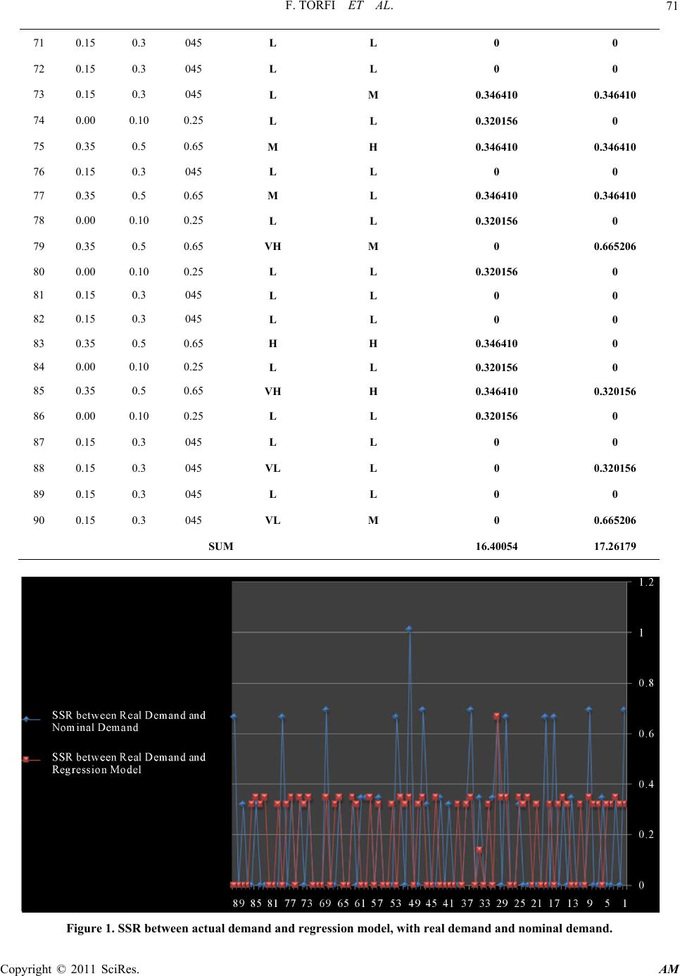

F. TORFI ET AL. 71
71 0.15 0.3 045 L L 0 0
72 0.15 0.3 045 L L 0 0
73 0.15 0.3 045 L M 0.346410 0.346410
74 0.00 0.10 0.25 L L 0.320156 0
75 0.35 0.5 0.65 M H 0.346410 0.346410
76 0.15 0.3 045 L L 0 0
77 0.35 0.5 0.65 M L 0.346410 0.346410
78 0.00 0.10 0.25 L L 0.320156 0
79 0.35 0.5 0.65 VH M 0 0.665206
80 0.00 0.10 0.25 L L 0.320156 0
81 0.15 0.3 045 L L 0 0
82 0.15 0.3 045 L L 0 0
83 0.35 0.5 0.65 H H 0.346410 0
84 0.00 0.10 0.25 L L 0.320156 0
85 0.35 0.5 0.65 VH H 0.346410 0.320156
86 0.00 0.10 0.25 L L 0.320156 0
87 0.15 0.3 045 L L 0 0
88 0.15 0.3 045 VL L 0 0.320156
89 0.15 0.3 045 L L 0 0
90 0.15 0.3 045 VL M 0 0.665206
SUM 16.40054 17.26179
Figure 1. SSR betwe en actual demand and regression model, with real demand and nominal de mand.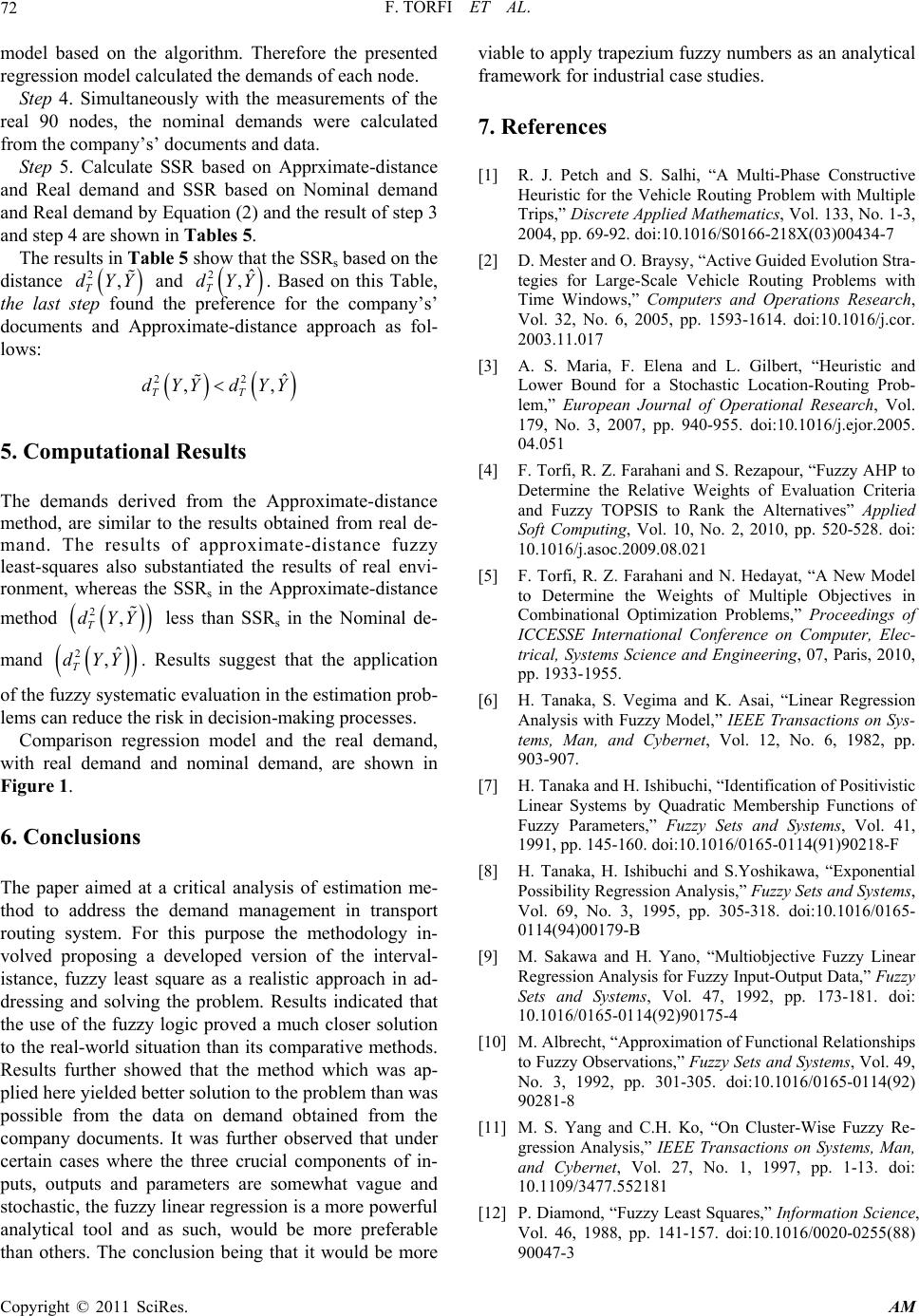

F. TORFI ET AL. 72
model based on the algorithm. Therefore the presented
regression model calculated the demands of each node.
Step 4. Simultaneously with the measurements of the
real 90 nodes, the nominal demands were calculated
from the company’s’ documents and data.
Step 5. Calculate SSR based on Apprximate-distance
and Real demand and SSR based on Nominal demand
and Real demand by Equation (2) and the result of step 3
and step 4 are shown in Tables 5.
The results in Table 5 show that the SSRs based on the
distance

2,
T
dYY
 and

2ˆ
,
T
dYY. Based on this Table,
the last step found the preference for the company’s’
documents and Approximate-distance approach as fol-
lows:
 
22
ˆ
,,
TT
dYY dYY

5. Computational Results
The demands derived from the Approximate-distance
method, are similar to the results obtained from real de-
mand. The results of approximate-distance fuzzy
least-squares also substantiated the results of real envi-
ronment, whereas the SSRs in the Approximate-distance
method
 
2,
T
dYY
 less than SSRs in the Nominal de-
mand


2ˆ
,
T
dYY. Results suggest that the application
of the fuzzy systematic evaluation in the estimation prob-
lems can reduce the risk in decision-making processes.
Comparison regression model and the real demand,
with real demand and nominal demand, are shown in
Figure 1.
6. Conclusions
The paper aimed at a critical analysis of estimation me-
thod to address the demand management in transport
routing system. For this purpose the methodology in-
volved proposing a developed version of the interval-
istance, fuzzy least square as a realistic approach in ad-
dressing and solving the problem. Results indicated that
the use of the fuzzy logic proved a much closer solution
to the real-world situation than its comparative methods.
Results further showed that the method which was ap-
plied here yielded better solution to the problem than was
possible from the data on demand obtained from the
company documents. It was further observed that under
certain cases where the three crucial components of in-
puts, outputs and parameters are somewhat vague and
stochastic, the fuzzy linear regression is a more powerful
analytical tool and as such, would be more preferable
than others. The conclusion being that it would be more
viable to apply trapezium fuzzy numbers as an analytical
framework for industrial case studies.
7. References
[1] R. J. Petch and S. Salhi, “A Multi-Phase Constructive
Heuristic for the Vehicle Routing Problem with Multiple
Trips,” Discrete Applied Mathematics, Vol. 133, No. 1-3,
2004, pp. 69-92. doi:10.1016/S0166-218X(03)00434-7
[2] D. Mester and O. Braysy, “Active Guided Evolution Stra-
tegies for Large-Scale Vehicle Routing Problems with
Time Windows,” Computers and Operations Research,
Vol. 32, No. 6, 2005, pp. 1593-1614. doi:10.1016/j.cor.
2003.11.017
[3] A. S. Maria, F. Elena and L. Gilbert, “Heuristic and
Lower Bound for a Stochastic Location-Routing Prob-
lem,” European Journal of Operational Research, Vol.
179, No. 3, 2007, pp. 940-955. doi:10.1016/j.ejor.2005.
04.051
[4] F. Torfi, R. Z. Farahani and S. Rezapour, “Fuzzy AHP to
Determine the Relative Weights of Evaluation Criteria
and Fuzzy TOPSIS to Rank the Alternatives” Applied
Soft Computing, Vol. 10, No. 2, 2010, pp. 520-528. doi:
10.1016/j.asoc.2009.08.021
[5] F. Torfi, R. Z. Farahani and N. Hedayat, “A New Model
to Determine the Weights of Multiple Objectives in
Combinational Optimization Problems,” Proceedings of
ICCESSE International Conference on Computer, Elec-
trical, Systems Science and Engineering, 07, Paris, 2010,
pp. 1933-1955.
[6] H. Tanaka, S. Vegima and K. Asai, “Linear Regression
Analysis with Fuzzy Model,” IEEE Transactions on Sys-
tems, Man, and Cybernet, Vol. 12, No. 6, 1982, pp.
903-907.
[7] H. Tanaka and H. Ishibuchi, “Identification of Positivistic
Linear Systems by Quadratic Membership Functions of
Fuzzy Parameters,” Fuzzy Sets and Systems, Vol. 41,
1991, pp. 145-160. doi:10.1016/0165-0114(91)90218-F
[8] H. Tanaka, H. Ishibuchi and S.Yoshikawa, “Exponential
Possibility Regression Analysis,” Fuzzy Sets and Systems,
Vol. 69, No. 3, 1995, pp. 305-318. doi:10.1016/0165-
0114(94)00179-B
[9] M. Sakawa and H. Yano, “Multiobjective Fuzzy Linear
Regression Analysis for Fuzzy Input-Output Data,” Fuzzy
Sets and Systems, Vol. 47, 1992, pp. 173-181. doi:
10.1016/0165-0114(92)90175-4
[10] M. Albrecht, “Approximation of Functional Relationships
to Fuzzy Observations,” Fuzzy Sets and Systems, Vol. 49,
No. 3, 1992, pp. 301-305. doi:10.1016/0165-0114(92)
90281-8
[11] M. S. Yang and C.H. Ko, “On Cluster-Wise Fuzzy Re-
gression Analysis,” IEEE Transactions on Systems, Man,
and Cybernet, Vol. 27, No. 1, 1997, pp. 1-13. doi:
10.1109/3477.552181
[12] P. Diamond, “Fuzzy Least Squares,” Information Science,
Vol. 46, 1988, pp. 141-157. doi:10.1016/0020-0255(88)
90047-3

F. TORFI ET AL. 73
[13] L. A. Zadeh, “Fuzzy Sets,” Information Control, Vol. 8,
1965, pp. 338-53. doi:10.1016/S0019-9958(65)90241-X
[14] T. Yang and H. Chih-Ching, “Multiple-Attribute Deci-
sion Making Methods for Plant Layout Design Problem,”
Robotics and computer-integrated manufacturing, Vol.
23, No. 1, 2007, pp. 126-137. doi:10.1016/j.rcim.2005.
12.002
[15] C. T. Chen, “Extensions of the TOPSIS for Group Deci-
sion-Making under Fuzzy Environment,” Fuzzy Sets and
Systems, Vol. 114, No. 1, 2000, pp. 1-9. doi:10.1016/
S0165-0114(97)00377-1
[16] M. S. Yang and T. S. Lin, “Fuzzy Least-Squares Linear
Regression Analysis for Fuzzy Input-Output Data,” Fuzzy
Sets and Systems, Vol. 126, No. 3, 2002, pp. 389-399.
doi:10.1016/S0165-0114(01)00066-5
[17] D. Dubois and H. Prade, “Fuzzy Sets and Systems:
Theory and Applications,” Academic Press, New York,
1980.