Journal of Signal and Information Processing, 2013, 4, 19-24
doi:10.4236/jsip.2013.43B004 Published Online August 2013 (http://www.scirp.org/journal/jsip) 19
Environmental Sound Recognition Using Double-Level
Energy Detection
Xiaoxia Zhang, Ying Li
College of Mathematics and Computer Science, Fuzhou University, Fuzhou, China.
Received April, 2013.
ABSTRACT
The performance of classic Mel-frequency cepstral coefficients (MFCC) is unsatisfactory in noisy environment with
different sound sources from nature. In this paper, a classification approach of the ecological environmental sounds us-
ing the double-level energy detection (DED) was presented. The DED was used to detect the existence of the sound
signals under noise conditions. In addition, MFCC features from the frames which were detected the presence of the
sound signals by DED were extracted. Ex perimental results show that the p roposed technology has better noise immu-
nity than classic MFCC, and also outperforms time-domain energy detection (TED) and frequency-domain energy de-
tection (FED) respectively.
Keywords: Ecological Environmental Sounds; Double-Level Energy Detection; Time-Domain Energy Detection;
Frequency-Domain Energy Detection; Mel-Frequency Cepstral Coefficients
1. Introduction
The sound recognition is a fundamental problem of the
sound signals processing. It has important applications in
many fields like media search [1], military [2], security
supervision [3] etc. Sound data contains a wealth of use-
ful information. Through the recognition and analysis of
sound, we can get lots of environmental characteristics,
such as climate, geography, time, species, etc. Sound can
get messages that the vision cannot capture. Moreover,
the sound can be obtained anytime and anywhere, it is
not limited to the light, and it is not necessary within the
field of vision. The required storage space is smaller than
that of the video signals. The sound data has many ad-
vantages.
In the practical application of sound , the soun d sources
are not clearly known, which lead to designing an appro-
priate sound signals detection method becomes more
difficult. En ergy detection does no t need to know a priori
knowledge of the sound signals and it is easy to imple-
ment. Therefore, the energy detection has a greater ad-
vantage in this case. The time-domain energy detection
(TED) runs faster, but the detection accuracy is not well,
while the frequency-domain energy detection (FED) has
higher detection accuracy, but runs more slowly. So we
construct the double-level energy detection (DED) by
combining the respective advantage of TED and FED.
Under the condition of guaranteeing certain detection
accuracy, this method is simple, effective and has lower
complexity than the separate use the time-domain or fre-
quency-domain energy detection.
The Mel-Frequency Cepstral Coefficients (MFCC) is
the most common feature used in many sound recogni-
tion systems [4]. The MFCC feature fully considers the
characteristics of human hearing, which has a good per-
formance in recognition. When MFCC is used to analyze
the sound signals with flat-spectrum noise, the effect is
not good, so the classification results of the MFCC de-
crease significantly in the background noise. To solve
this abuse, we combine DED with MFCC. This method
has a certain degree of noise immunity, and the feature
vector is denoted as DED_MFCC. As the model created
by SVM shows more robust, we extract the DED_MFCC
to train the SVM classifier.
This paper is organized as follows. Section 2 presents
the principles of DED. Section 3 introduces the feature
extraction process and section 4 introduces the classifica-
tion approach. In section 5, the experimental setup and
the achieved results are presented. Finally, the conclusion
of our work is given in section 6.
2. Double-Level Energy Detection
The energy detector is a kind of ideal signals detection
tools, which can detect the existence of the sound signals
in the noise environment. At present, energy detection
can be divided into time-domain energy detection (TED)
and frequency-domain energy detection (FED). These

Environmental Sound Recognition Using Double-Level Energy Detection
20
two methods have their own respective strengths and
weaknesses [5]. TED has the advantages including rela-
tively simple, short running time, but disadvantage of
low accuracy of the sound signal detection. Because of
the discrete fast Fourier transform (FFT), FED can im-
prove the application flexibility and accuracy of detec-
tion, but the running speed slows down.
Given the advantages and disadvantages of the two
methods described above, we use TED to detect the ob-
servation sound signals firstly, if there are no sound sig-
nals being detected, indicating that the sound is the noise;
otherwise, we use FED to detect the observation sound
signals, if it cannot detect the sound signals, it can be
concluded that the observation sound signals do not con-
tain sound signals, on the contrary, w e can determine the
observation sound signals contain the sound signals. The
flow of DED is illustrated in Figure 1. Under the condi-
tion of guaranteeing certain detection accuracy, this
method is simple, effective and has lower complexity
than the separate use the time-domain or frequency do-
main energy detection.
Figure 1. Flow of DED.
2.1. Time-Domain Energy Detection
The principle of time-domain energy detection [6-8] is
shown in Figure 2. Where Y(n) is the observation vecto r,
2
w

is the noise variance,

is the threshold that is set for
a specific probability of false alarm (PFA). Y(n) goes
2
w

Figure 2. Time-domain energy detection.
through the operations of modulus square and accumula-
tion as:


2
()
n
TYn

(1)
The judgment form ul a i n Figure 1 is
1
0
2
H
wH
T




(2)
if 2
w
T


, the sound signals exist; if 2
w
T



, the
sound signals do not exist.
In Equation (2), H0 means the sound signals do not ex-
ist, while H1 means the observation vector contains the
sound signals. So the entire detection process is the hy-
pothesis of a binary t e st:
0
1
()
() () ()
Wn H
Yn Sn WnH



= (3)
where n = 1,…, N, N is the number of samples.
This work uses a pre-given probability of false alarm
(PFA), and the test statistic can be approximated by a
Gaussian distribution:
24
022 222
1
(,2)
(( ,2( ))
ww
ws ws
HNormalNN
HNormalN N

  
:T～，
:T～ (4)
where N is the number of samples (detection time, its
value equals to the length of the frame), 2
w

is the noise
variance, 2
s

is the sound signa l s vari ance.
When the signals do not exist, through the known
probability of false alarm (PFA), we can obtain the
threshold of the judgment. In the case of H0, T is in line
with the Gaussian distribution, so the PFA is:
0
2|
w
T
PFA PH 






(5)
then
2
N
Q PFA
N
  


 (6)
where

2
1exp 2
2x
y
Qx dy





.
Therefore, through the given N and PFA, the threshold
can be obtained by Equat i on ( 6):

Environmental Sound Recognition Using Double-Level Energy Detection 21
1
2(NNQPFA 

 ) (7)
It can be seen from the above analysis, for the given
PFA and the noise variance, we can calculate the judg-
ment threshold, and then we can conclude that which
frame contains the sou nd signals by Equat i on ( 2).
2.2. Frequency-Domain Energy Detection
The principle of frequency-domain energy detection is
shown in Figure 3.
2
w

Figure 3. Frequency-domain energy detection.
Compared to the time-domain energy detection, fre-
quency-domain energy detection firstly puts the observa-
tion vector through the FFT module to transform the
time-domain signals into the frequency-domain signals.
Then get the frequency-domain energy by putting the
frequency domain signals through the modules of squar-
ing and accumulating. Finally, compare the value of the
frequency domain energy which is divided by noise vari-
ance with the threshold, which determines whether there
are sound signals. If the probability of TED is P, when the
observation signals contain the sound signals actually, the
omission probability is 1-P after the comparison with the
threshold. If the TED determines that there are the sound
signals in the obs ervation signals, th en start F ED to detect
the unknown s ou nds.
3. Extraction of DED_MFCC
MFCC analyzes sound signals from the perspective of the
human ear frequency level of the nonlinear psychological
sense. It uses a nonlinear Mel-frequency scale to simulate
the human auditory system. Values of the Mel-frequency
scale are roughly logarithmic with the linear frequency,
and more in line with the human auditory cha racteristics.
The calculation of MFCC parameters is based on the
frequency reference of “bark” [9]. The relationship with
the frequency conversion is:
10
2595log (1)
700
mel
f
f
(8)
The energy detection method does not have the pre-
processing of pre-emphasis. We simply divide the sound
signals into frames and inter-frame without overlap,
which thereby greatly enhances the efficiency of running.
In this paper, the process of DED_MFCC extraction is
shown in Figure 4.
Figure 4. Extraction of DED_MFCC.
The steps of extracting DED_MFCC are as follows:
1) The input sound is divided into successive frames,
256 sample s per frame, inter-frame wit hout o verl ap.
2) Each frame is coupled with the Hanning window,
then discard the frames without the sound signals though
the TED.
3) Fast Fourier Transform is applied to the frame, then
use the FED to discard the frames which is the false posi-
tives by the TED.
4) The energy spectrum generated from the FED passes
through a set of the triangular Mel-scale filter bank, and
the output is (),1,2, ,ml lL

. L is set to 24. The
span of each triangular filter in the Mel-scale is equal, and
it is set to 112Mel.
5) Take the logarithm of all of the filter output, then
apply the Discrete Cosine Transform (DCT) to get a
group of DED_MFCC:
1
1
_()log()cos{()},0
2
L
l
j
dedmfccjm lljL
L





(9)
In this paper, we use the first 12 coefficients as DED_
MFCC.
4. SVM Classification Algorithm
The support vector machine (SVM) is first proposed by
Cortes and Vapnik etc. It shows many unique advantages
in solving the problems of the small samples, nonlinear
and high dimensional pattern recognition. SVM is built
on the basis of VC dimension theory and structural risk
minimization of the statistical learning theory. The basic
principle is to correctly separate the two sample po ints in
the separating hyperplane, and to maximize the minimum
distance of the plus or minus class samples to the sepa-
rating hyperplane.
Assume that {x1,x2,…,xl}is the training sample,
{y1,y2,…,yl} is the corresponding class label. SVM finds
the separating hyperplane with the largest interval by
solving the following quadratic programming prob- lem:
(,,)1
1
min 2
..[] 10
0,1,2,3, ,
n
Ti
wb i
T
ii i
i
ww C
styw xb
in










(10)
where C is a coefficient that regulates the value between
the misclassification and the robustness of the classifica-

Environmental Sound Recognition Using Double-Level Energy Detection
22
tion (width of margin).
Many linearly inseparable problems in the real world
can be converted into linearly separable by mapping to
high-dimensional space with the SVM kernel function
[10]. At present, the most commonly used kernel func-
tions include linear kernel, polynomial kernel, RBF ker-
nel and sigmoid kernel. In the experiment of this paper,
we use the LIBSVM package which is designed by DR.
Lin Zhiren of Taiwan University.
5. Experiments
5.1. Experimental Setup
The sounds of the ecological environment which are used
in these experiments are the variety of birds singing.
There is a total of 12 kinds of birds singing here including
flour chicken, Zhu turtledove, Dong chicken, male thrush,
blackwater chicken, hair chicken, mother partridge,
mountain turtledove, water rails, white-eye, the mother
pheasant, mother bamboo chicken. There are 20 samples
of each kind of birds singing, of which 10 samples are
used for training and 10 samples for testing, so a total of
240 sound samples. These bird singings were recorded by
voice recorder in the outdoors, and the length of each
sound sample is more than two seco nds, the sampling rate
is 44100 Hz. In this work, the sign al to noise ratio (SNR)
of the sounds which is used to train the SVM models is
60 dB in the training step, which is done by adding the
noise at 60 dB SNR to the clear sound data. In the testing
step, we use the sounds with different SNRs. The ex-
tracted features include classic MFCC, TED_MFCC (use
the time-domain energy detection only), FED_MFCC
(use the frequency-domain energy detection only) and
DED_MFCC, and they are all 12-dimensional feature
vectors. The kernel function used in SVM is RBF kernel.
The PFA was set to .
8
10
5.2. Evaluation Results
In order to observe the noise immunity of the DED_
MFCC feature on the ecological environment sounds
classification, we use SVM to construct the classification
models based on MFCC, TED_MFCC, FED_MFCC and
DED_MFCC respectively. We use 30 frames of each
sample for training, and 256 frames of each sample for
testing. Here, the no ise we add to the clear bird singing is
the white Gaussian noise. The classification accuracy of
the test samples corresponding to the different SNRs is
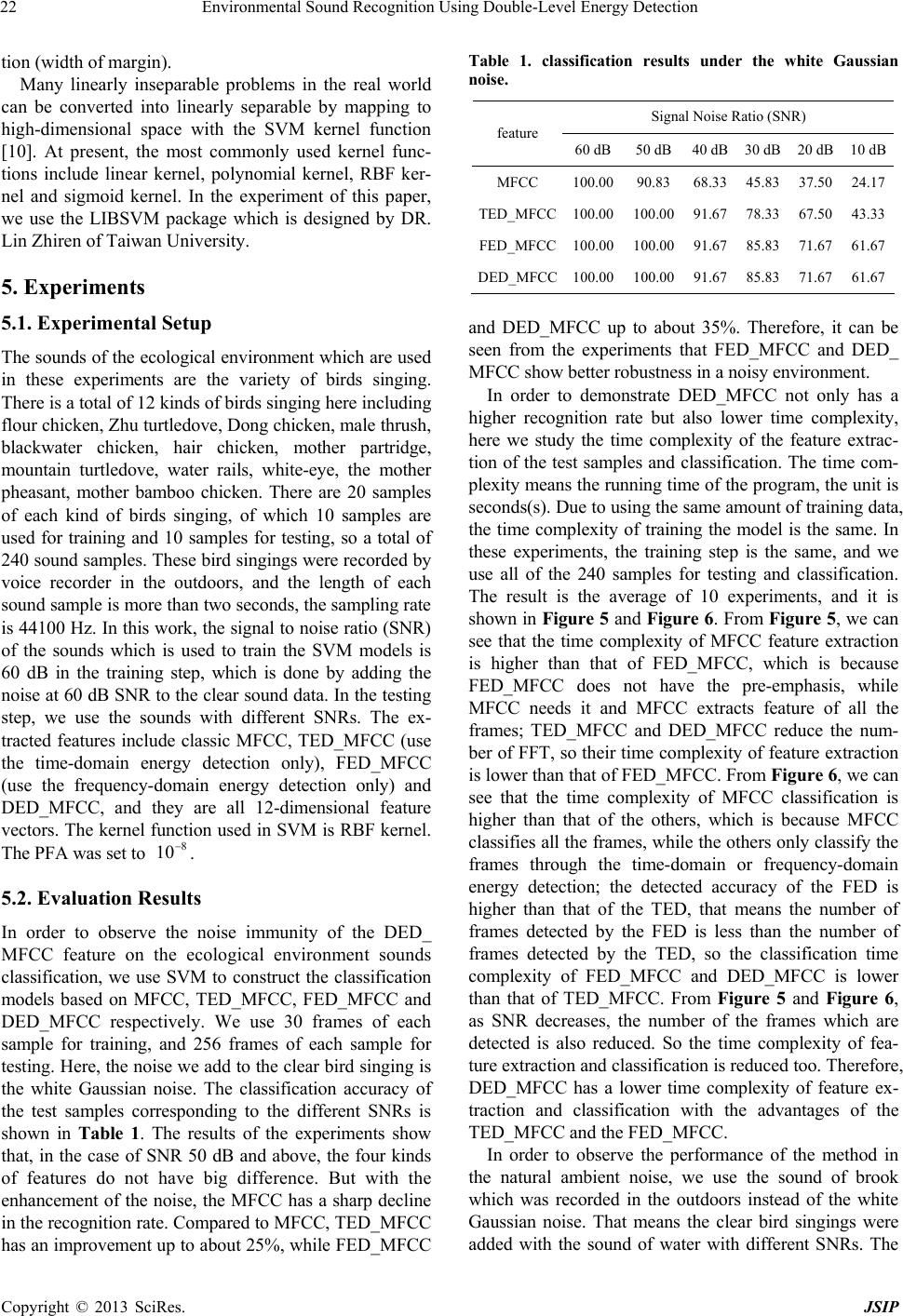
shown in Table 1. The results of the experiments show
that, in the case of SNR 50 dB and above, the four kinds
of features do not have big difference. But with the
enhancement of the noise, the MFCC has a sharp decline
in the recognition rate. Compar ed to MFCC, TED_MFCC
has an improvement up to about 25%, while FED_MFCC
Table 1. classification results under the white Gaussian
noise.
Signal Noise Ratio (SNR)
feature 60 dB50 dB40 dB 30 dB 20 dB10 dB
MFCC 100.0090.8368.33 45.83 37.5024.17
TED_MFCC 100.00100.0091.67 78.33 67.5043.33
FED_MFCC100.00100.0091.67 85.83 71.6761.67
DED_MFCC 100.00100.0091.67 85.83 71.6761.67
and DED_MFCC up to about 35%. Therefore, it can be
seen from the experiments that FED_MFCC and DED_
MFCC show bett e r robust nes s i n a noisy environm ent .
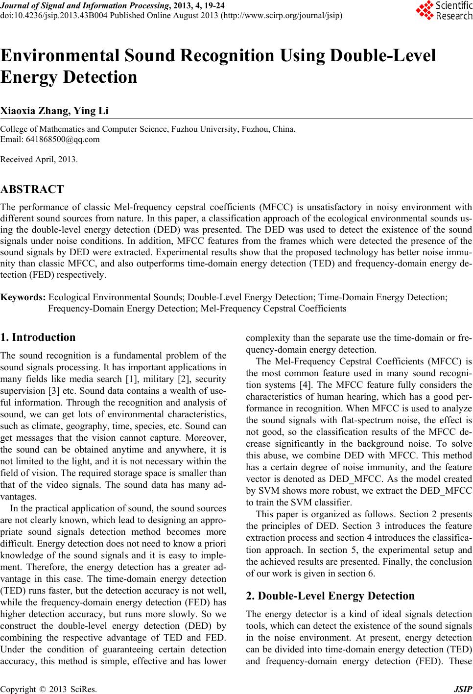
In order to demonstrate DED_MFCC not only has a
higher recognition rate but also lower time complexity,
here we study the time complexity of the feature extrac-
tion of the test samples and classification. The time com-
plexity means t he running time o f the program, the u nit is
seconds(s). Due to using the same amount of training data,
the time complexity of training the model is the same. In
these experiments, the training step is the same, and we
use all of the 240 samples for testing and classification.
The result is the average of 10 experiments, and it is
shown in Figure 5 and Figure 6. From Figure 5, we can
see that the time complexity of MFCC feature extraction
is higher than that of FED_MFCC, which is because
FED_MFCC does not have the pre-emphasis, while
MFCC needs it and MFCC extracts feature of all the
frames; TED_MFCC and DED_MFCC reduce the num-
ber of FFT, so their time complexity of feature extraction
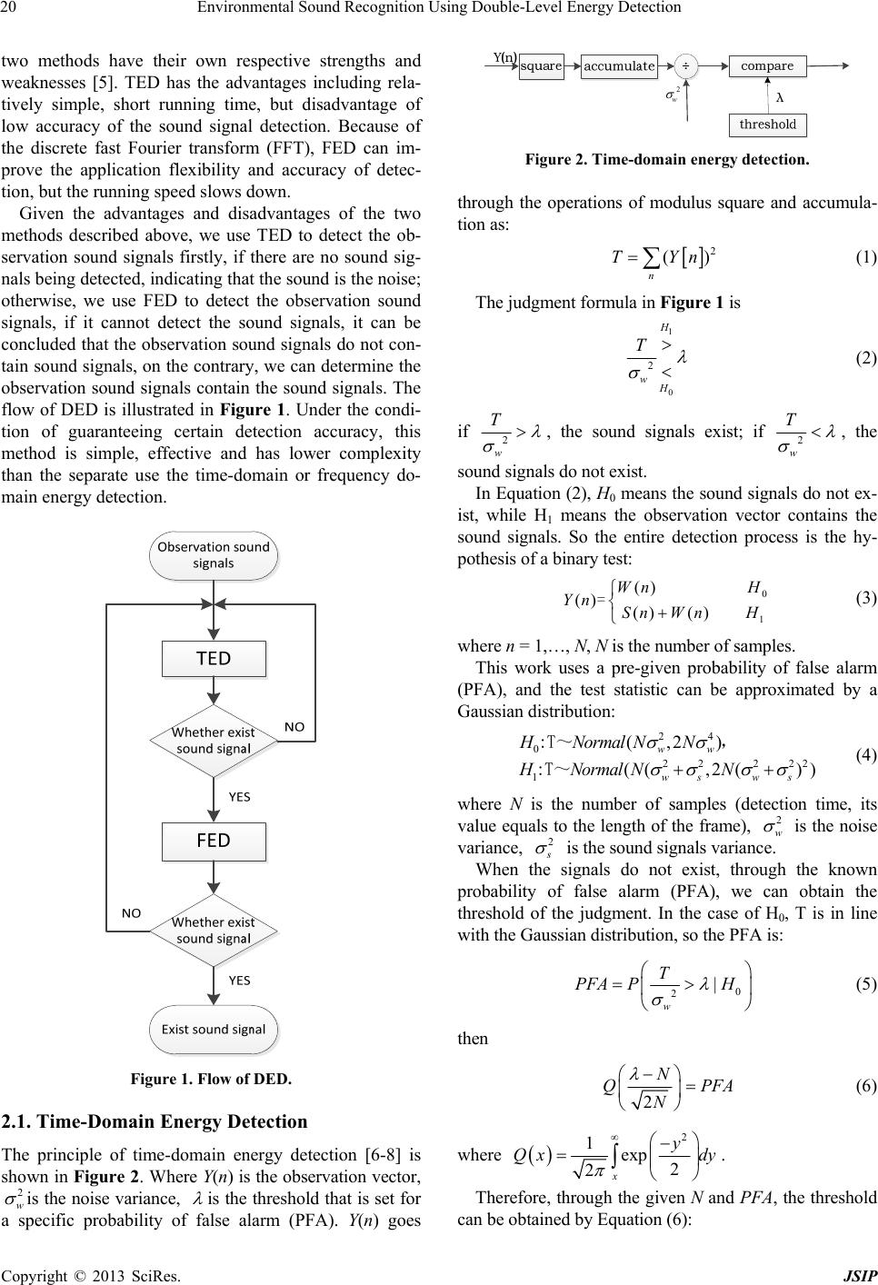
is lower than that of FED_ MFCC. From Fi gure 6, we can
see that the time complexity of MFCC classification is
higher than that of the others, which is because MFCC
classifies all the frames, while the others only classify the
frames through the time-domain or frequency-domain
energy detection; the detected accuracy of the FED is
higher than that of the TED, that means the number of
frames detected by the FED is less than the number of
frames detected by the TED, so the classification time
complexity of FED_MFCC and DED_MFCC is lower
than that of TED_MFCC. From Figure 5 and Figure 6,
as SNR decreases, the number of the frames which are
detected is also reduced. So the time complexity of fea-
ture extraction and classification is reduced too. Therefore,
DED_MFCC has a lower time complexity of feature ex-
traction and classification with the advantages of the
TED_MFCC and the FED_MFCC.
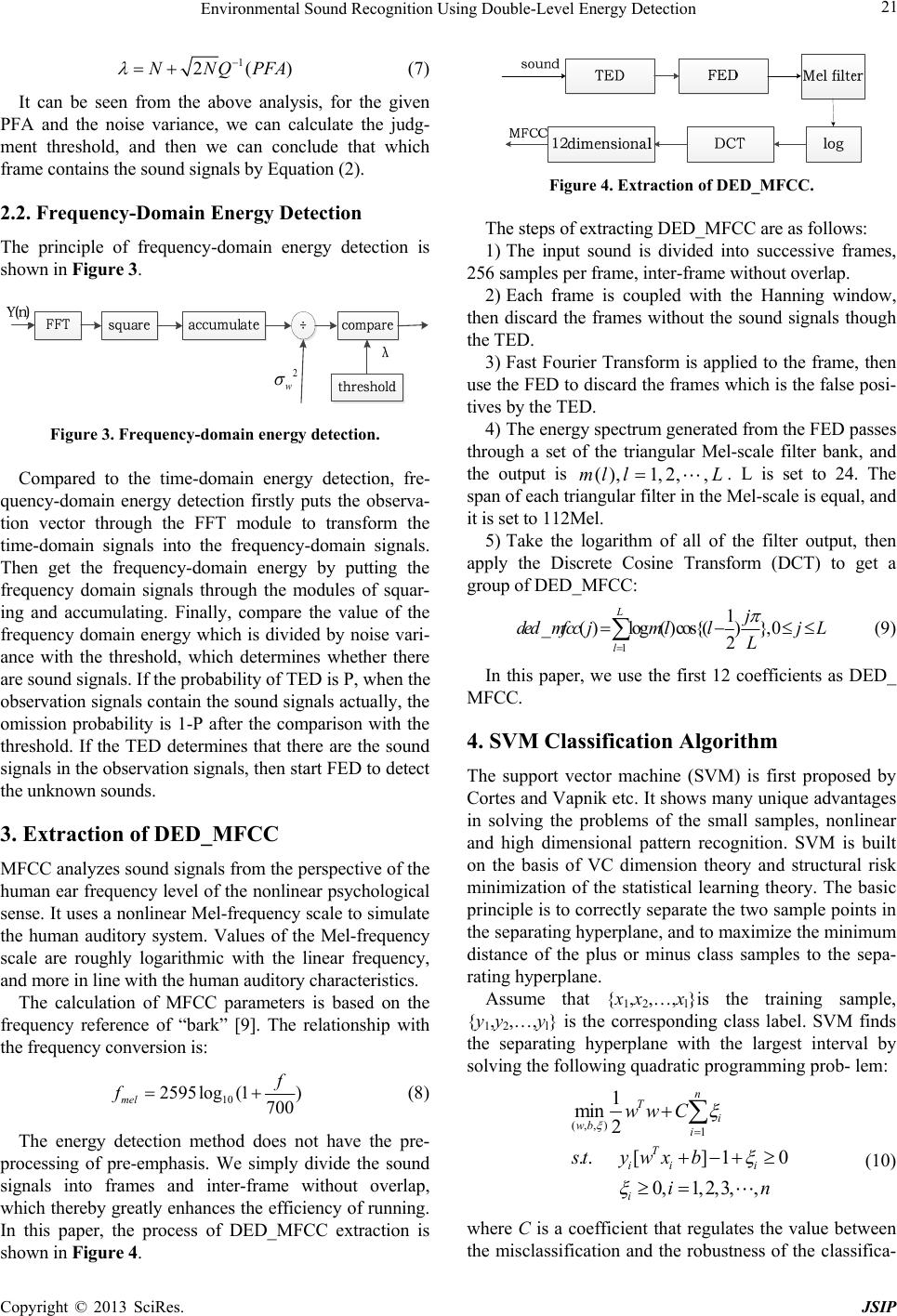
In order to observe the performance of the method in
the natural ambient noise, we use the sound of brook
which was recorded in the outdoors instead of the white
Gaussian noise. That means the clear bird singings were
added with the sound of water with different SNRs. The

Environmental Sound Recognition Using Double-Level Energy Detection 23
Figure 5. Feature extraction time complexity under the
Gaussian white noise.
Figure 6. Classification time complexity under the Gaussian
white noise.
results are shown in Table 2. From these experiments, we
can see that this method is applicable to not only the
white Gaussian noise in the simulative laboratory condi-
tions, but also the noise of the natural environment. And
when the SNR is below 30 dB, the classification results
are even better than those of the white Gaussian noise.
6. Conclusions and Future Work
In this paper, we present a feature extraction method of
MFCC based on double level energy detector. The ex-
perimental results show that the classification result is
slightly better than the classic MFCC in the case of the
high SNRs; but in the case of low SNRs, this method has
good robustness, and the classification accuracy has
greatly improved compared with the classic MFCC. In
terms of the time complexity, the proposed method com-
bines the advantages of the time-domain energy detection
and the frequency-domain energy detection, so it has
Table 2. classification results under the noise of the natural
environment.
Signal Noise Ratio (SNR)
feature 60dB50dB40dB 30dB 20dB10dB
MFCC 100.0091.6780.83 49.17 39.1724.17
TED_MFCC100.00100.0091.67 78.33 70.8361.67
FED_MFCC100.00100.0091.67 85.33 73.3365.83
DED_MFCC100.00100.0091.67 85.83 73.3365.83
lower time complexity in both the process of feature ex-
traction and classification. In addition, it performs better
in the natural ambient noise than in the Gaussian white
noise. There are two disadvantages in the proposed
method: first of all, the recognition rate is still less than
ideal in the case of low SNRs; second, the sound of the
ecological environment is limited to birds singing. In the
future works, we will look for new features which have
better noise immunity combined with this proposed
method to improve the classification effect, and cover
more kinds of ecol ogi cal environmental sounds.
7. Acknowledgements
This work is supported by the National Natural Science
Fund Project (No. 61075022).
REFERENCES
[1] R. Typke, F. Wiering and R. Veltkamp, “A Survey of
Music Information Retrieval Systems,” Proceedings of
the 6th International Conference on Music Information
Retrieval (ISMIR 2005), London, 11-15 September 2005,
pp. 153-160.
[2] L. Gerosa, G. Valenzise and M. Tagliasacchi, et al.,
“Scream and Gunshot Detection in Noisy Environments,”
Proceedings of the 15th European Signal Processing
Conference (EUSIPCO 2007), Poznan, 3-7 September
2007, pp. 1216-1220.
[3] C. Zieger, A. Bruti and P. Svaizer, “Acoustic Based Sur-
veillance System for Intrusion Detection,” Proceedings of
the 6th IEEE International Conference on Advanced
Video and Signal Based Surveillance (AVSS 2009), Genoa,
2-4 September 2009, pp. 314-319.
doi:10.1109/AVSS.2009.49
[4] A. Dufaux, “Detection and Recognition of Impulsive
Sounds Signals,” Institute de Microtechnique Neuchatel,
Switzerland, 2001.
[5] M. Q. Wu, W. Ma and C. X. Xu, “A Low-Power Algo-
rithm of Uniting the Time-Domain and Fre-
quency-Domain Thresholds,” China Patent, No.
101848044, 2010.
[6] H. Urknowitz, “Energy Detection of Unknown Determi-
nistic Signals,” Proceedings of the IEEE, Vol. 55, No. 4,
1967, pp. 523-531. doi:10.1109/PROC.1967.5573

Environmental Sound Recognition Using Double-Level Energy Detection
24
[7] L. Vergara, J. Mora gues, J. Gosalbez, et al., “Detection of
Signals of Unknown Duration by Multiple Energy De-
tectors,” Signal Processing, Vol. 90, No. 2, 2010, pp.
719-726. doi:10.1016/j.sigpro.2009.08.007
[8] S. M. Kay, “Fundamentals of Statistical Signal Process-
ing: Detection Theory,” 1st Edition, New Jersey: Pren-
tice-Hall, 1998.
[9] Y. Li, “A Quick Classification for Area Environmental
Audio Data Based on Local Search Tree,” Proceedings of
the 2009 International Conference on Environmental
Science and Information Application Technology (ESIAT
2009), Wuhan, China, 4-5 July 2009, pp. 569 -574.
doi:10.1109/ESIAT.2009.15
[10] V. David and A. Sánchez, “Advanced Support Vector
Machines and Kernel Methods,” Neurocomputing, Vol.
55, No. 1-2, 2003, pp. 5-20.
doi:10.1016/S0925-2312(03)00373-4.