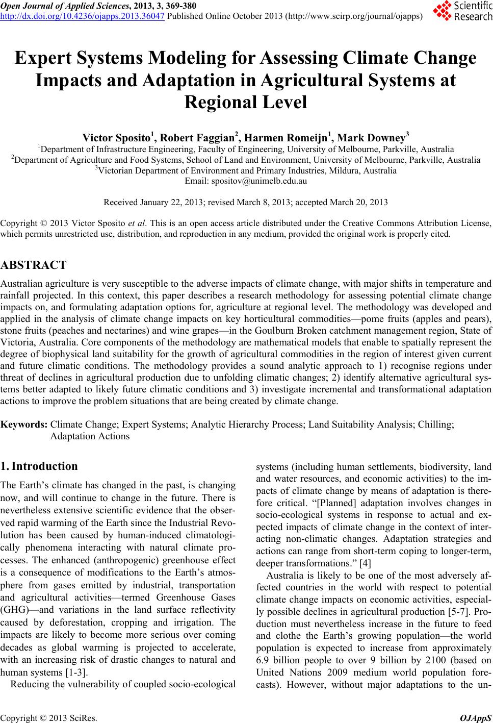
 Open Journal of Applied Sciences, 2013, 3, 369-380 http://dx.doi.org/10.4236/ojapps.2013.36047 Published Online October 2013 (http://www.scirp.org/journal/ojapps) Expert Systems Modeling for Assessing Climate Change Impacts and Adaptation in Agricultural Systems at Regional Level Victor Sposito1, Robert Faggian2, Harmen Romeijn1, Mark Downey3 1Department of Infrastructure Engineering, Faculty of Engineering, University of Melbourne, Parkville, Australia 2Department of Agriculture and Food Systems, School of Land and Environment, University of Melbourne, Parkville, Australia 3Victorian Department of Environment and Primary Industries, Mildura, Australia Email: spositov@unimelb.edu.au Received January 22, 2013; revised March 8, 2013; accepted March 20, 2013 Copyright © 2013 Victor Sposito et al. This is an open access article distributed under the Creative Commons Attribution License, which permits unrestricted use, distribution, and reproduction in any medium, provided the original work is properly cited. ABSTRACT Australian agriculture is very susceptible to the adverse impacts of climate change, with major shifts in temperature and rainfall projected. In this context, this paper describes a research methodology for assessing potential climate change impacts on, and formulating adaptation options for, agriculture at regional level. The methodology was developed and applied in the analysis of climate change impacts on key horticultural commodities—pome fruits (apples and pears), stone fruits (peaches and nectarines) and wine grapes—in the Goulburn Broken catchment management region, State of Victoria, Australia. Core components of the methodology are mathematical models that enable to spatially represent the degree of biophysical land suitability for the growth of agricultural commodities in the region of interest given current and future climatic conditions. The methodology provides a sound analytic approach to 1) recognise regions under threat of declines in agricultural production due to unfolding climatic changes; 2) identify alternative agricultural sys- tems better adapted to likely future climatic conditions and 3) investigate incremental and transformational adaptation actions to improve the problem situations that are being created by climate change. Keywords: Climate Change; Expert Systems; Analytic Hierarchy Process; Land Suitability Analysis; Chilling; Adaptation Actions 1. Introduction The Earth’s climate has changed in the past, is changing now, and will continue to change in the future. There is nevertheless extensive scientific evidence that the obser- ved rapid warming of the Earth since the Industrial Revo- lution has been caused by human-induced climatologi- cally phenomena interacting with natural climate pro- cesses. The enhanced (anthropogenic) greenhouse effect is a consequence of modifications to the Earth’s atmos- phere from gases emitted by industrial, transportation and agricultural activities—termed Greenhouse Gases (GHG)—and variations in the land surface reflectivity caused by deforestation, cropping and irrigation. The impacts are likely to become more serious over coming decades as global warming is projected to accelerate, with an increasing risk of drastic changes to natural and human systems [1-3]. Reducing the vulnerability of coupled socio-ecological systems (including human settlements, biodiversity, land and water resources, and economic activities) to the im- pacts of climate change by means of adaptation is there- fore critical. “[Planned] adaptation involves changes in socio-ecological systems in response to actual and ex- pected impacts of climate change in the context of inter- acting non-climatic changes. Adaptation strategies and actions can range from short-term coping to longer-term, deeper transformations.” [4] Australia is likely to be one of the most adversely af- fected countries in the world with respect to potential climate change impacts on economic activities, especial- ly possible declines in agricultural production [5-7]. Pro- duction must nevertheless increase in the future to feed and clothe the Earth’s growing population—the world population is expected to increase from approximately 6.9 billion people to over 9 billion by 2100 (based on United Nations 2009 medium world population fore- casts). However, without major adaptations to the un- C opyright © 2013 SciRes. OJAppS 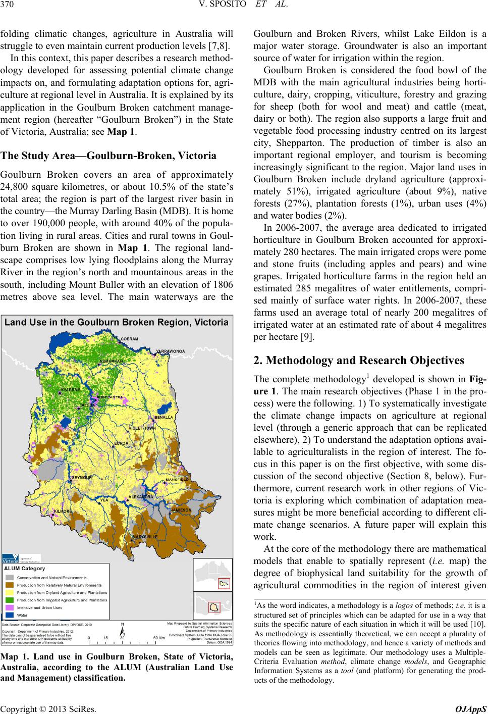 V. SPOSITO ET AL. 370 folding climatic changes, agriculture in Australia will struggle to even maintain current production levels [7,8]. In this context, this paper describes a research method- ology developed for assessing potential climate change impacts on, and formulating adaptation options for, agri- culture at regional level in Australia. It is explained by its application in the Goulburn Broken catchment manage- ment region (hereafter “Goulburn Broken”) in the State of Victoria, Australia; see Map 1. The Study Area—Goulburn-Broken, Victoria Goulburn Broken covers an area of approximately 24,800 square kilometres, or about 10.5% of the state’s total area; the region is part of the largest river basin in the country—the Murray Darling Basin (MDB). It is home to over 190,000 people, with around 40% of the popula- tion living in rural areas. Cities and rural towns in Goul- burn Broken are shown in Map 1. The regional land- scape comprises low lying floodplains along the Murray River in the region’s north and mountainous areas in the south, including Mount Buller with an elevation of 1806 metres above sea level. The main waterways are the Map 1. Land use in Goulburn Broken, State of Victoria, Australia, according to the ALUM (Australian Land Use and Management) classification. Goulburn and Broken Rivers, whilst Lake Eildon is a major water storage. Groundwater is also an important source of water for irrigation within the region. Goulburn Broken is considered the food bowl of the MDB with the main agricultural industries being horti- culture, dairy, cropping, viticulture, forestry and grazing for sheep (both for wool and meat) and cattle (meat, dairy or both). The region also supports a large fruit and vegetable food processing industry centred on its largest city, Shepparton. The production of timber is also an important regional employer, and tourism is becoming increasingly significant to the region. Major land uses in Goulburn Broken include dryland agriculture (approxi- mately 51%), irrigated agriculture (about 9%), native forests (27%), plantation forests (1%), urban uses (4%) and water bodies (2%). In 2006-2007, the average area dedicated to irrigated horticulture in Goulburn Broken accounted for approxi- mately 280 hectares. The main irrigated crops were pome and stone fruits (including apples and pears) and wine grapes. Irrigated horticulture farms in the region held an estimated 285 megalitres of water entitlements, compri- sed mainly of surface water rights. In 2006-2007, these farms used an average total of nearly 200 megalitres of irrigated water at an estimated rate of about 4 megalitres per hectare [9]. 2. Methodology and Research Objectives The complete methodology1 developed is shown in Fig- ure 1. The main research objectives (Phase 1 in the pro- cess) were the following. 1) To systematically investigate the climate change impacts on agriculture at regional level (through a generic approach that can be replicated elsewhere), 2) To understand the adaptation options avai- lable to agriculturalists in the region of interest. The fo- cus in this paper is on the first objective, with some dis- cussion of the second objective (Section 8, below). Fur- thermore, current research work in other regions of Vic- toria is exploring which combination of adaptation mea- sures might be more beneficial according to different cli- mate change scenarios. A future paper will explain this work. At the core of the methodology there are mathematical models that enable to spatially represent (i.e. map) the degree of biophysical land suitability for the growth of agricultural commodities in the region of interest given 1As the word indicates, a methodology is a logos of methods; i.e.it is a structured set of principles which can be adapted for use in a way that suits the specific nature of each situation in which it will be used [10]. As methodology is essentially theoretical, we can accept a plurality o theories flowing into methodology, and hence a variety of methods and models can be seen as legitimate. Our methodology uses a Multiple- Criteria Evaluation method, climate change models, and Geographic Information Systems as a tool (and platform) for generating the prod- ucts of the methodology. Copyright © 2013 SciRes. OJAppS 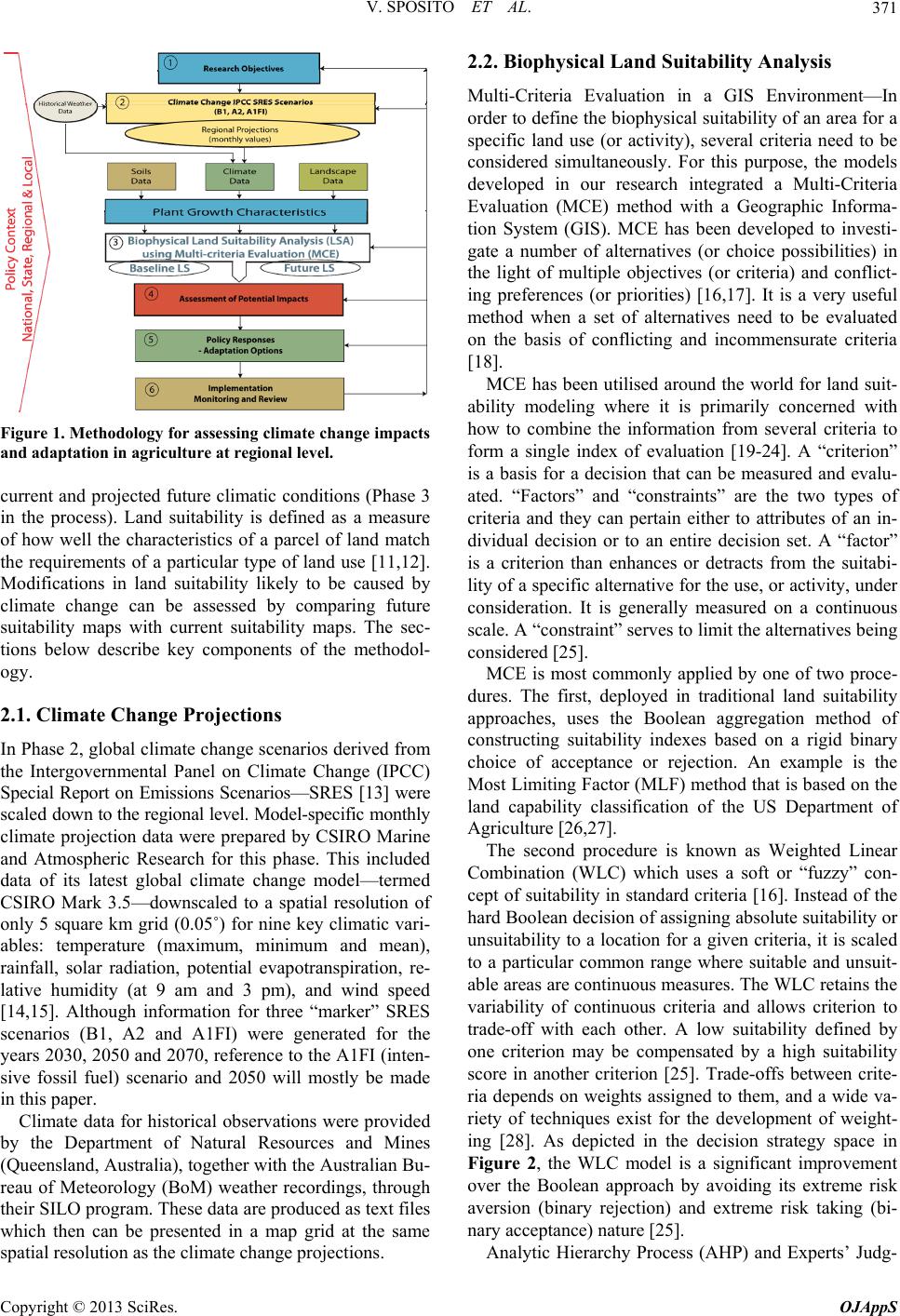 V. SPOSITO ET AL. 371 Figure 1. Methodology for assessing climate change impacts and adaptation in agriculture at regional level. current and projected future climatic conditions (Phase 3 in the process). Land suitability is defined as a measure of how well the characteristics of a parcel of land match the requirements of a particular type of land use [11,12]. Modifications in land suitability likely to be caused by climate change can be assessed by comparing future suitability maps with current suitability maps. The sec- tions below describe key components of the methodol- ogy. 2.1. Climate Change Projections In Phase 2, global climate change scenarios derived from the Intergovernmental Panel on Climate Change (IPCC) Special Report on Emissions Scenarios—SRES [13] were scaled down to the regional level. Model-specific monthly climate projection data were prepared by CSIRO Marine and Atmospheric Research for this phase. This included data of its latest global climate change model—termed CSIRO Mark 3.5—downscaled to a spatial resolution of only 5 square km grid (0.05˚) for nine key climatic vari- ables: temperature (maximum, minimum and mean), rainfall, solar radiation, potential evapotranspiration, re- lative humidity (at 9 am and 3 pm), and wind speed [14,15]. Although information for three “marker” SRES scenarios (B1, A2 and A1FI) were generated for the years 2030, 2050 and 2070, reference to the A1FI (inten- sive fossil fuel) scenario and 2050 will mostly be made in this paper. Climate data for historical observations were provided by the Department of Natural Resources and Mines (Queensland, Australia), together with the Australian Bu- reau of Meteorology (BoM) weather recordings, through their SILO program. These data are produced as text files which then can be presented in a map grid at the same spatial resolution as the climate change projections. 2.2. Biophysical Land Suitability Analysis Multi-Criteria Evaluation in a GIS Environment—In order to define the biophysical suitability of an area for a specific land use (or activity), several criteria need to be considered simultaneously. For this purpose, the models developed in our research integrated a Multi-Criteria Evaluation (MCE) method with a Geographic Informa- tion System (GIS). MCE has been developed to investi- gate a number of alternatives (or choice possibilities) in the light of multiple objectives (or criteria) and conflict- ing preferences (or priorities) [16,17]. It is a very useful method when a set of alternatives need to be evaluated on the basis of conflicting and incommensurate criteria [18]. MCE has been utilised around the world for land suit- ability modeling where it is primarily concerned with how to combine the information from several criteria to form a single index of evaluation [19-24]. A “criterion” is a basis for a decision that can be measured and evalu- ated. “Factors” and “constraints” are the two types of criteria and they can pertain either to attributes of an in- dividual decision or to an entire decision set. A “factor” is a criterion than enhances or detracts from the suitabi- lity of a specific alternative for the use, or activity, under consideration. It is generally measured on a continuous scale. A “constraint” serves to limit the alternatives being considered [25]. MCE is most commonly applied by one of two proce- dures. The first, deployed in traditional land suitability approaches, uses the Boolean aggregation method of constructing suitability indexes based on a rigid binary choice of acceptance or rejection. An example is the Most Limiting Factor (MLF) method that is based on the land capability classification of the US Department of Agriculture [26,27]. The second procedure is known as Weighted Linear Combination (WLC) which uses a soft or “fuzzy” con- cept of suitability in standard criteria [16]. Instead of the hard Boolean decision of assigning absolute suitability or unsuitability to a location for a given criteria, it is scaled to a particular common range where suitable and unsuit- able areas are continuous measures. The WLC retains the variability of continuous criteria and allows criterion to trade-off with each other. A low suitability defined by one criterion may be compensated by a high suitability score in another criterion [25]. Trade-offs between crite- ria depends on weights assigned to them, and a wide va- riety of techniques exist for the development of weight- ing [28]. As depicted in the decision strategy space in Figure 2, the WLC model is a significant improvement over the Boolean approach by avoiding its extreme risk aversion (binary rejection) and extreme risk taking (bi- nary acceptance) nature [25]. Analytic Hierarchy Process (AHP) and Experts’ Judg- Copyright © 2013 SciRes. OJAppS  V. SPOSITO ET AL. 372 Figure 2. Decision strategy space. Source: [23, p. 17]. ment—In our research, the MCE was implemented using an Expert Systems Modeling—the Analytic Hierarchy Process (AHP) developed by Saaty [29,30]. AHP pro- vides a framework that incorporates experts’ participa- tion in the decision-making process. Compared to empi- rical models based purely on the correlation amongst data, this Expert Systems Modeling incorporates the knowledge of experts who can address significant issues and have an understanding of the system of concern that may be relevant to the required decision-making. The method is also better suited when the availability of good data is limited. As explained by Saaty [30], “basically the AHP is a method of breaking down a complex unstructured situa- tion into its component parts; arranging these parts, or variables, into a hierarchical order [or decision tree]; as- signing numerical values to subjective judgments on the relative importance of each variable; and synthesizing the judgments to determine which variables have the highest priority and should be acted upon to influence the out- come of the situation. AHP incorporates both the qualita- tive and the quantitative aspects of human thought: the qualitative to define the problem and its hierarchy and the quantitative to express judgments and preferences concisely. The process itself is designed to integrate these dual properties.” When AHP is integrated with GIS, it can deal with criteria that are interdependent, both from the effect on land and in the interaction between spatial units [31]. It is required when using a WLC in MCE that the weights sum to one. In the AHP, the weights are calcu- lated by taking the principal eigenvector of a square re- ciprocal matrix of pair-wise comparisons between the criteria. All possible pairs of criteria are compared by experts on a 9-point continuous scale for their relative importance to determining the suitability of the stated objectives. The ratings are then introduced in a matrix to calculate the weights. The accuracy of the weight results at each level of the AHP hierarchy depends on the con- sistency of judgments in the pair-wise comparisons. A consistency ratio (CR) measures the logical inconsis- tency of judgments and enables the identification of pos- sible errors in the matrix. If CR ≥ 0.10 the pair-wise comparison matrix must be reformulated [25,29,30]. 3. Example of a Biophysical Land Suitability Model (LSA) The methodology was developed and applied in the ana- lysis of the potential climate change impacts on key hor- ticultural commodities—pome fruits (apples and pears), stone fruits (peaches and nectarines) and wine grapes—in Goulburn Broken [30]. However, for illustration purpo- ses, we explain only the LSA model for apples (Royal Gala variety—the most common in Australia). This model was developed in a workshop-type situa- tion held during approximately 6 hours with participation of a large group of experts including: land use and envi- ronmental planners, natural resource analysts/managers, climate and soil scientists, hydrologists, geographers, and agriculturalists involved in pome fruits cultivation. Rele- vant material was distributed prior to the workshop com- prising information on the methodology, particularly on the AHP, climate, soil, topography, and scientific cri- teria for the growth of the crop being examined. At the commencement of the workshop, the agenda for the day was discussed, and explanations on the methodology and available data (including gaps and accuracy) were pro- vided. A workshop Facilitator assisted in the develop- ment of the following steps in model formulation 1) con- struction of the AHP hierarchy, 2) making pair-wise comparisons and 3) calculating the priorities. To under- take these steps on-the-fly, we used a computer program developed by us. It is interesting to note that, in general, there was agreement in relation to weights and ratings, and, if there was disagreement, the experts with the greatest knowledge on the factor in question ultimately prevailed. Much discussion occurred in relation to the weightings at the top of the AHP hierarchy, especially between soils and climate; (as expected) the soil scien- tists argued that soil was the most important factor influ- encing pome fruits growth. A counter-argument was however put that climate, on account of its significant projected changes should be given a greater weight; and this position was finally accepted. The apple LSA model was developed setting a goal to produce a yield within a range (as agreed at the work- shop) of 30 to 60 tonnes per hectare per year (t/ha/y). These are desirable values on the assumption that the agricultural land is utilised to its maximum potential through Best Management Practices (BMP). Current yields, as reported by the Australian Bureau of Statistics (ABS), show that the average production of all current orchards in Goulburn Broken is at the lower range of the stated yields at around 33 t/ha/y. And Figure 3 shows the overall structure of the model and the landscape branch’s hierarchy. Because of its significance for this paper, of the other two branches of the LSA model—soil and cli- Copyright © 2013 SciRes. OJAppS 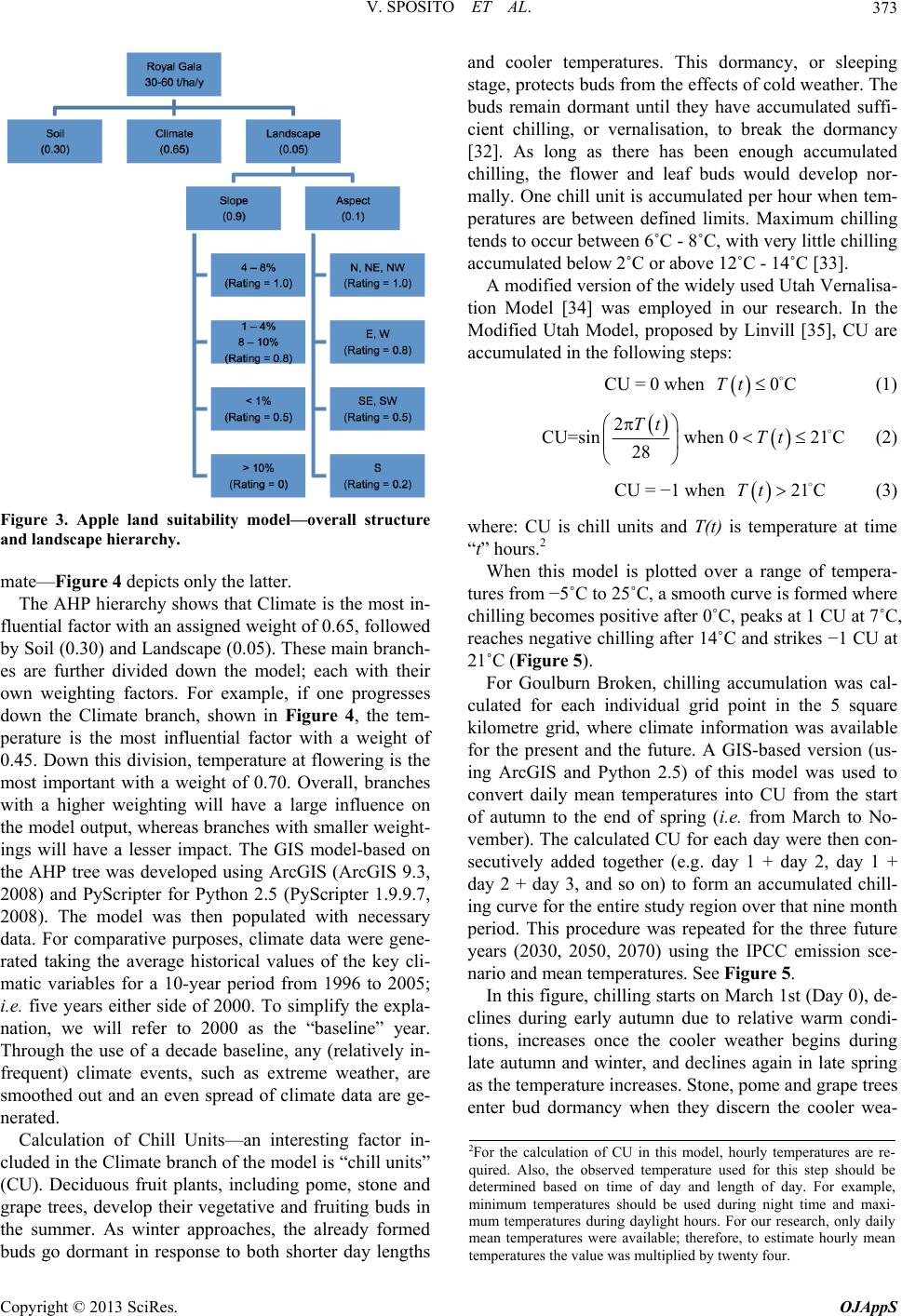 V. SPOSITO ET AL. 373 Figure 3. Apple land suitability model—overall structure and landscape hierarc hy. mate—Figure 4 depicts only the latter. The AHP hierarchy shows that Climate is the most in- fluential factor with an assigned weight of 0.65, followed by Soil (0.30) and Landscape (0.05). These main branch- es are further divided down the model; each with their own weighting factors. For example, if one progresses down the Climate branch, shown in Figure 4, the tem- perature is the most influential factor with a weight of 0.45. Down this division, temperature at flowering is the most important with a weight of 0.70. Overall, branches with a higher weighting will have a large influence on the model output, whereas branches with smaller weight- ings will have a lesser impact. The GIS model-based on the AHP tree was developed using ArcGIS (ArcGIS 9.3, 2008) and PyScripter for Python 2.5 (PyScripter 1.9.9.7, 2008). The model was then populated with necessary data. For comparative purposes, climate data were gene- rated taking the average historical values of the key cli- matic variables for a 10-year period from 1996 to 2005; i.e. five years either side of 2000. To simplify the expla- nation, we will refer to 2000 as the “baseline” year. Through the use of a decade baseline, any (relatively in- frequent) climate events, such as extreme weather, are smoothed out and an even spread of climate data are ge- nerated. Calculation of Chill Units—an interesting factor in- cluded in the Climate branch of the model is “chill units” (CU). Deciduous fruit plants, including pome, stone and grape trees, develop their vegetative and fruiting buds in the summer. As winter approaches, the already formed buds go dormant in response to both shorter day lengths and cooler temperatures. This dormancy, or sleeping stage, protects buds from the effects of cold weather. The buds remain dormant until they have accumulated suffi- cient chilling, or vernalisation, to break the dormancy [32]. As long as there has been enough accumulated chilling, the flower and leaf buds would develop nor- mally. One chill unit is accumulated per hour when tem- peratures are between defined limits. Maximum chilling tends to occur between 6˚C - 8˚C, with very little chilling accumulated below 2˚C or above 12˚C - 14˚C [33]. A modified version of the widely used Utah Vernalisa- tion Model [34] was employed in our research. In the Modified Utah Model, proposed by Linvill [35], CU are accumulated in the following steps: CU = 0 when (1) 0CTt 2 CU=sinwhen021 C 28 Tt Tt (2) CU = −1 when (3) 21 CTt where: CU is chill units and T(t) is temperature at time “t” hours.2 When this model is plotted over a range of tempera- tures from −5˚C to 25˚C, a smooth curve is formed where chilling becomes positive after 0˚C, peaks at 1 CU at 7˚C, reaches negative chilling after 14˚C and strikes −1 CU at 21˚C (Figure 5). For Goulburn Broken, chilling accumulation was cal- culated for each individual grid point in the 5 square kilometre grid, where climate information was available for the present and the future. A GIS-based version (us- ing ArcGIS and Python 2.5) of this model was used to convert daily mean temperatures into CU from the start of autumn to the end of spring (i.e. from March to No- vember). The calculated CU for each day were then con- secutively added together (e.g. day 1 + day 2, day 1 + day 2 + day 3, and so on) to form an accumulated chill- ing curve for the entire study region over that nine month period. This procedure was repeated for the three future years (2030, 2050, 2070) using the IPCC emission sce- nario and mean temperatures. See Figure 5. In this figure, chilling starts on March 1st (Day 0), de- clines during early autumn due to relative warm condi- tions, increases once the cooler weather begins during late autumn and winter, and declines again in late spring as the temperature increases. Stone, pome and grape trees enter bud dormancy when they discern the cooler wea- 2For the calculation of CU in this model, hourly temperatures are re- quired. Also, the observed temperature used for this step should be determined based on time of day and length of day. For example, minimum temperatures should be used during night time and maxi- mum temperatures during daylight hours. For our research, only daily mean temperatures were available; therefore, to estimate hourly mean temperatures the value was multiplied by twenty four. Copyright © 2013 SciRes. OJAppS 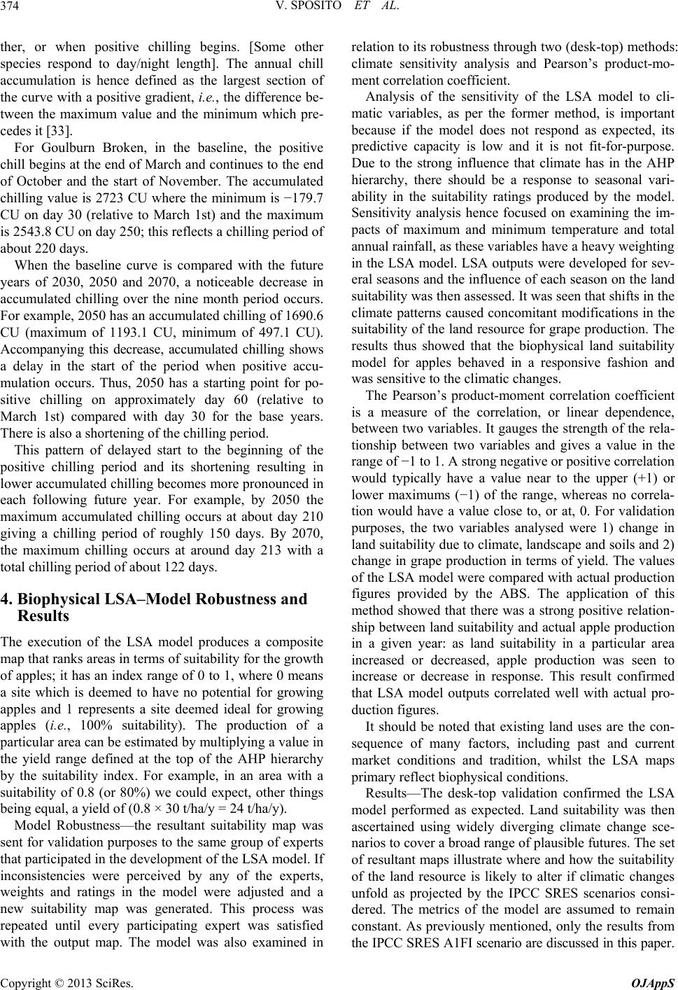 V. SPOSITO ET AL. 374 ther, or when positive chilling begins. [Some other species respond to day/night length]. The annual chill accumulation is hence defined as the largest section of the curve with a positive gradient, i.e., the difference be- tween the maximum value and the minimum which pre- cedes it [33]. For Goulburn Broken, in the baseline, the positive chill begins at the end of March and continues to the end of October and the start of November. The accumulated chilling value is 2723 CU where the minimum is −179.7 CU on day 30 (relative to March 1st) and the maximum is 2543.8 CU on day 250; this reflects a chilling period of about 220 days. When the baseline curve is compared with the future years of 2030, 2050 and 2070, a noticeable decrease in accumulated chilling over the nine month period occurs. For example, 2050 has an accumulated chilling of 1690.6 CU (maximum of 1193.1 CU, minimum of 497.1 CU). Accompanying this decrease, accumulated chilling shows a delay in the start of the period when positive accu- mulation occurs. Thus, 2050 has a starting point for po- sitive chilling on approximately day 60 (relative to March 1st) compared with day 30 for the base years. There is also a shortening of the chilling period. This pattern of delayed start to the beginning of the positive chilling period and its shortening resulting in lower accumulated chilling becomes more pronounced in each following future year. For example, by 2050 the maximum accumulated chilling occurs at about day 210 giving a chilling period of roughly 150 days. By 2070, the maximum chilling occurs at around day 213 with a total chilling period of about 122 days. 4. Biophysical LSA–Model Robustness and Results The execution of the LSA model produces a composite map that ranks areas in terms of suitability for the growth of apples; it has an index range of 0 to 1, where 0 means a site which is deemed to have no potential for growing apples and 1 represents a site deemed ideal for growing apples (i.e., 100% suitability). The production of a particular area can be estimated by multiplying a value in the yield range defined at the top of the AHP hierarchy by the suitability index. For example, in an area with a suitability of 0.8 (or 80%) we could expect, other things being equal, a yield of (0.8 × 30 t/ha/y = 24 t/ha/y). Model Robustness—the resultant suitability map was sent for validation purposes to the same group of experts that participated in the development of the LSA model. If inconsistencies were perceived by any of the experts, weights and ratings in the model were adjusted and a new suitability map was generated. This process was repeated until every participating expert was satisfied with the output map. The model was also examined in relation to its robustness through two (desk-top) methods: climate sensitivity analysis and Pearson’s product-mo- ment correlation coefficient. Analysis of the sensitivity of the LSA model to cli- matic variables, as per the former method, is important because if the model does not respond as expected, its predictive capacity is low and it is not fit-for-purpose. Due to the strong influence that climate has in the AHP hierarchy, there should be a response to seasonal vari- ability in the suitability ratings produced by the model. Sensitivity analysis hence focused on examining the im- pacts of maximum and minimum temperature and total annual rainfall, as these variables have a heavy weighting in the LSA model. LSA outputs were developed for sev- eral seasons and the influence of each season on the land suitability was then assessed. It was seen that shifts in the climate patterns caused concomitant modifications in the suitability of the land resource for grape production. The results thus showed that the biophysical land suitability model for apples behaved in a responsive fashion and was sensitive to the climatic changes. The Pearson’s product-moment correlation coefficient is a measure of the correlation, or linear dependence, between two variables. It gauges the strength of the rela- tionship between two variables and gives a value in the range of −1 to 1. A strong negative or positive correlation would typically have a value near to the upper (+1) or lower maximums (−1) of the range, whereas no correla- tion would have a value close to, or at, 0. For validation purposes, the two variables analysed were 1) change in land suitability due to climate, landscape and soils and 2) change in grape production in terms of yield. The values of the LSA model were compared with actual production figures provided by the ABS. The application of this method showed that there was a strong positive relation- ship between land suitability and actual apple production in a given year: as land suitability in a particular area increased or decreased, apple production was seen to increase or decrease in response. This result confirmed that LSA model outputs correlated well with actual pro- duction figures. It should be noted that existing land uses are the con- sequence of many factors, including past and current market conditions and tradition, whilst the LSA maps primary reflect biophysical conditions. Results—The desk-top validation confirmed the LSA model performed as expected. Land suitability was then ascertained using widely diverging climate change sce- narios to cover a broad range of plausible futures. The set of resultant maps illustrate where and how the suitability of the land resource is likely to alter if climatic changes unfold as projected by the IPCC SRES scenarios consi- dered. The metrics of the model are assumed to remain constant. As previously mentioned, only the results from the IPCC SRES A1FI scenario are discussed in this paper. Copyright © 2013 SciRes. OJAppS 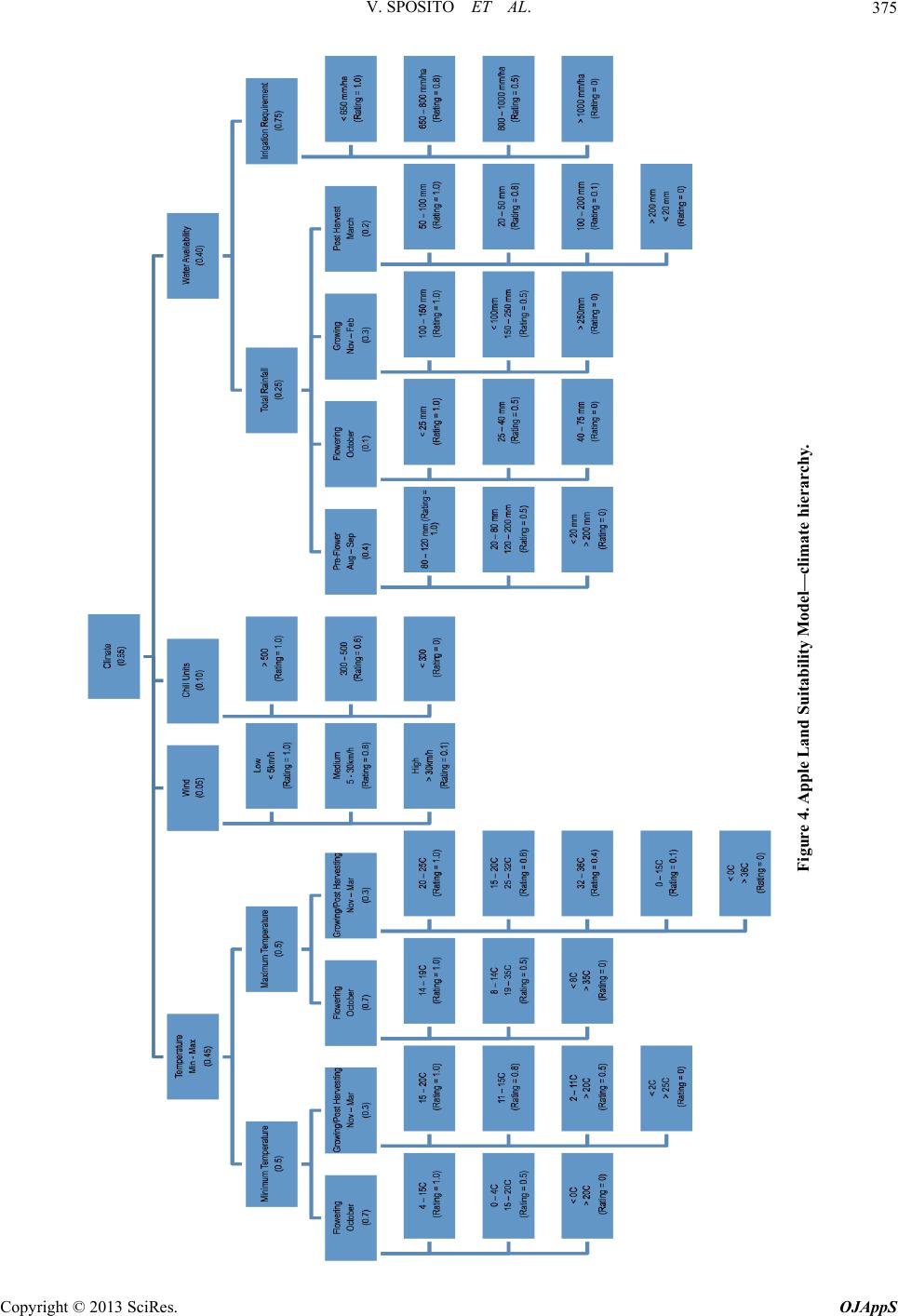 V. SPOSITO ET AL. Copyright © 2013 SciRes. OJAppS 375 Figure 4. Apple Land Suitability Model—climate hierarchy.  V. SPOSITO ET AL. 376 Accumulated Chilling from M arch 1st to November 30th 0000 2543. 770191 -179.65397 6 1911. 265987 -418.929931 1193.1429 26 -497.417736 -615.250193 371.98986 1 -750 -500 -250 0 250 500 750 1000 1250 1500 1750 2000 2250 2500 2750 0306091121 152183 213244 274 Day number f r om M arch 1st Accumul at ed Chil ling ( CU) Base 2030 2050 2070 Figure 5. Accumulated chilling from March 1st to November 30th. CU refers to chill units; Base refers to the years 1996 to 2005. Maps 2-4 show, respectively, the results of LSA for the baseline (average climatic conditions in the period 1996- 2005; noted as year 2000), year 2050 and the change in land suitability between these two years. Red, orange, yellow and green colours in Maps 2 and 3 and associated legends represent, respectively, very low (0% to 10%), low (20% to 40%), moderate (50% to 70%) and high (80% to 100% suitability) ranges. A large area in the south (shown in grey colour in the maps) and portions of the northwest and east of the region are restricted to pro- tect native vegetation and other natural landscapes. Map 2 shows that most areas in Goulburn Broken are currently high in suitability to produce 30 - 60 t/ha/y of apples. Only a small scattering of areas show a moderate suitability; in particular, areas between Numurkah and Shepparton and north of Kyabram display this ranking. Map 3 for 2050 depicts a large change in the land suit- ability for apples from the high to the moderate catego- ries. The northern regional areas (north of the town of Euroa) have shifted from a high land suitability category to moderate land suitability ranges. In the southern re- gional areas, land suitability has changed from the high suitability categories of 90% and 100% to the high suit- ability category of 80%. These changes are largely a consequence of the projected increases in temperature and concomitant decreases in rainfall across the region. In the comparison between the baseline and 2050 (Map 4), a decrease indicates that there has been a 10% change from a higher suitability class to a lower suitabi- lity class (e.g. from 90% to 80%); similarly an increase indicates that there has been a 10% change from a lower class to a higher class (e.g. from 80% to 90%). A high increase denotes that there has been a 20% change from a low suitability class to a higher suitability class and a high decrease indicates that there has been a 20% reduc- tion from a higher suitability class. No change means that there has been no variation between the baseline and the year of the comparison. Therefore, from the baseline to the year 2050 changes are quite pronounced with over half of the region displaying a decrease in land suitability. This is primarily seen in the areas south of the town of Euroa. If a new variety of apples (or any commodity) is better adapted to the likely future climatic conditions, a new LSA model can be developed and parameterised with new weights (based on the new data) to investigate whether an anticipated improvement in performance will actually occur. 5. Discussion The integration of MCE methods, particularly the AHP, with GIS is fairly well established in theory and practice in the analysis of land uses [18-24]. The linking of the AHP with climate change projections to determine pos- sible changes in agricultural land suitability as a conse- quence of potential climate change, we believe, a novelty of the methodology outlined in this paper. It proved Copyright © 2013 SciRes. OJAppS 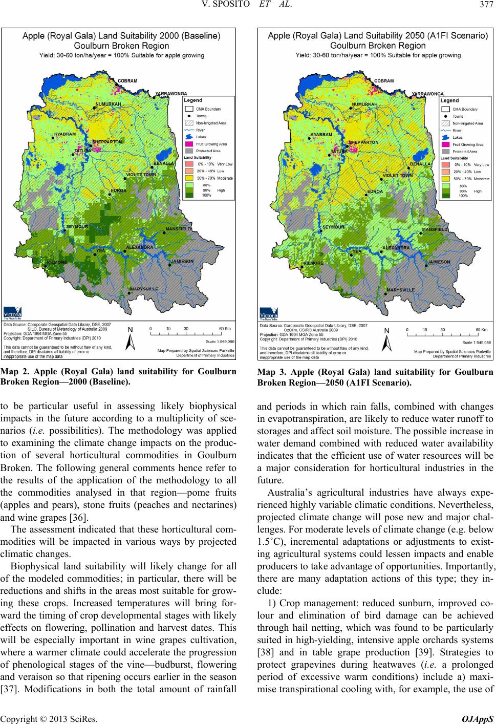 V. SPOSITO ET AL. 377 Map 2. Apple (Royal Gala) land suitability for Goulburn Broken Region—2000 (Baseline). to be particular useful in assessing likely biophysical impacts in the future according to a multiplicity of sce- narios (i.e. possibilities). The methodology was applied to examining the climate change impacts on the produc- tion of several horticultural commodities in Goulburn Broken. The following general comments hence refer to the results of the application of the methodology to all the commodities analysed in that region—pome fruits (apples and pears), stone fruits (peaches and nectarines) and wine grapes [36]. The assessment indicated that these horticultural com- modities will be impacted in various ways by projected climatic changes. Biophysical land suitability will likely change for all of the modeled commodities; in particular, there will be reductions and shifts in the areas most suitable for grow- ing these crops. Increased temperatures will bring for- ward the timing of crop developmental stages with likely effects on flowering, pollination and harvest dates. This will be especially important in wine grapes cultivation, where a warmer climate could accelerate the progression of phenological stages of the vine—budburst, flowering and veraison so that ripening occurs earlier in the season [37]. Modifications in both the total amount of rainfall Map 3. Apple (Royal Gala) land suitability for Goulburn Broken Region—2050 (A1FI Scenario). and periods in which rain falls, combined with changes in evapotranspiration, are likely to reduce water runoff to storages and affect soil moisture. The possible increase in water demand combined with reduced water availability indicates that the efficient use of water resources will be a major consideration for horticultural industries in the future. Australia’s agricultural industries have always expe- rienced highly variable climatic conditions. Nevertheless, projected climate change will pose new and major chal- lenges. For moderate levels of climate change (e.g. below 1.5˚C), incremental adaptations or adjustments to exist- ing agricultural systems could lessen impacts and enable producers to take advantage of opportunities. Importantly, there are many adaptation actions of this type; they in- clude: 1) Crop management: reduced sunburn, improved co- lour and elimination of bird damage can be achieved through hail netting, which was found to be particularly suited in high-yielding, intensive apple orchards systems [38] and in table grape production [39]. Strategies to protect grapevines during heatwaves (i.e. a prolonged period of excessive warm conditions) include a) maxi- mise transpirational cooling with, for example, the use of Copyright © 2013 SciRes. OJAppS 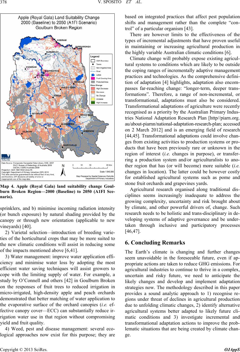 V. SPOSITO ET AL. 378 Map 4. Apple (Royal Gala) land suitability change Goul- burn Broken Region—2000 (Baseline) to 2050 (A1FI Sce- nario). sprinklers, and b) minimise incoming radiation intensity (or bunch exposure) by natural shading provided by the canopy or through new orientation (applicable to new vineyards) [40]. 2) Varietal selection—introduction of breeding varie- ties of the horticultural crops that may be more suited to the new climatic conditions will assist in reducing some of the impacts mentioned above [6,41]. 3) Water management: improve water application effi- ciency and minimise water loss by adopting the most efficient water saving techniques will assist growers to cope with the limiting supply of water. For example, a study by O’Connell and others [42] in Goulburn Broken on the responses of fruit trees to reduced irrigation in micro-irrigated, high-density apple and peach orchards demonstrated that better matching of water application to the evaporative surface of the orchard canopies (i.e. ef- fective canopy cover—ECC) can substantially reduce ir- rigation water use in that region without compromising yield and fruit quality. 4) Weed, pest and disease management: several eco- logical approaches now exist for this purpose; they are based on integrated practices that affect pest population shifts and management rather than the complete “con- trol” of a particular organism [43]. There are however limits to the effectiveness of the types of incremental adjustments that have proven useful in maintaining or increasing agricultural production in the highly variable Australian climatic conditions [6]. Climate change will probably expose existing agricul- tural systems to conditions which are likely to be outside the coping ranges of incrementally adaptive management practices and technologies. As the comprehensive defini- tion of adaptation [4] highlights, adaptation also encom- passes far-reaching change: “longer-term, deeper trans- formations”. Therefore, a range of non-incremental, or transformational, adaptations must also be considered. Transformational adaptations of agriculture were recently recognised as a priority by the Australian Primary Indus- tries National Adaptation Research Plan [http//piarn.org. au/about-piarnn/national-adaptation-research-plan; accessed on 2 March 2012] and is an emerging field of research [44,45]. Transformational adaptations could involve chan- ges from existing activities to production systems or pro- ducts that have been previously rare or unknown in the region of interest (i.e. changes in purpose), or transfer- ring a production system and/or agriculturalists to ano- ther region that has (or will become) more suitable (i.e. changes in location). The latter could be however costly for established agricultural systems such as pome and stone fruit orchards and grapevines yards. Agricultural research organised along traditional dis- ciplines seems increasingly inadequate to address the growing complexity, uncertainty and risk brought about by climate, and other powerful drivers of, change. Such research needs to be holistic and trans-disciplinary in de- veloping systems of adaptive governance and be under- taken through inclusive and participatory processes [46,47]. 6. Concluding Remarks The Earth’s climate is changing and further changes seem unavoidable in the foreseeable future, even if ap- propriate actions are taken to reduce GHG emissions. For agricultural industries to continue to thrive in a complex, uncertain and risky future, we need to anticipate the likely changes and develop and implement adaptation strategies now. The methodology described in this paper provides a sound analytic approach to 1) recognise re- gions under threat of declines in agricultural production due to unfolding climatic changes, 2) identify alternative agricultural systems better adapted to likely future cli- matic conditions and 3) investigate incremental and transformational adaptation actions to improve the prob- lematic situations that are being created by climate chan- ge. Copyright © 2013 SciRes. OJAppS 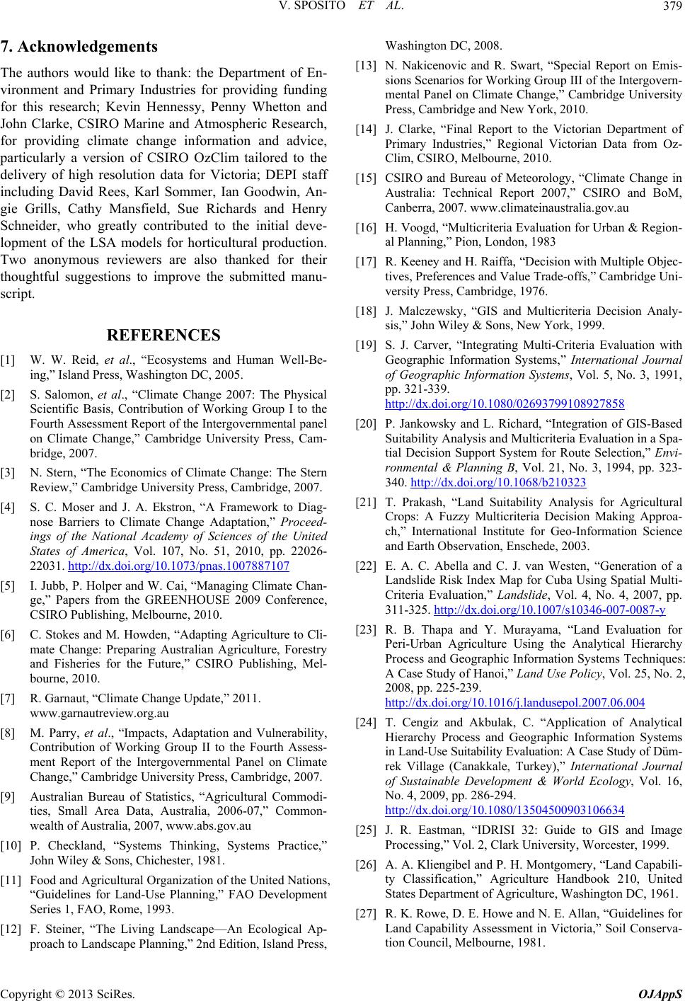 V. SPOSITO ET AL. 379 7. Acknowledgements The authors would like to thank: the Department of En- vironment and Primary Industries for providing funding for this research; Kevin Hennessy, Penny Whetton and John Clarke, CSIRO Marine and Atmospheric Research, for providing climate change information and advice, particularly a version of CSIRO OzClim tailored to the delivery of high resolution data for Victoria; DEPI staff including David Rees, Karl Sommer, Ian Goodwin, An- gie Grills, Cathy Mansfield, Sue Richards and Henry Schneider, who greatly contributed to the initial deve- lopment of the LSA models for horticultural production. Two anonymous reviewers are also thanked for their thoughtful suggestions to improve the submitted manu- script. REFERENCES [1] W. W. Reid, et al., “Ecosystems and Human Well-Be- ing,” Island Press, Washington DC, 2005. [2] S. Salomon, et al., “Climate Change 2007: The Physical Scientific Basis, Contribution of Working Group I to the Fourth Assessment Report of the Intergovernmental panel on Climate Change,” Cambridge University Press, Cam- bridge, 2007. [3] N. Stern, “The Economics of Climate Change: The Stern Review,” Cambridge University Press, Cambridge, 2007. [4] S. C. Moser and J. A. Ekstron, “A Framework to Diag- nose Barriers to Climate Change Adaptation,” Proceed- ings of the National Academy of Sciences of the United States of America, Vol. 107, No. 51, 2010, pp. 22026- 22031. http://dx.doi.org/10.1073/pnas.1007887107 [5] I. Jubb, P. Holper and W. Cai, “Managing Climate Chan- ge,” Papers from the GREENHOUSE 2009 Conference, CSIRO Publishing, Melbourne, 2010. [6] C. Stokes and M. Howden, “Adapting Agriculture to Cli- mate Change: Preparing Australian Agriculture, Forestry and Fisheries for the Future,” CSIRO Publishing, Mel- bourne, 2010. [7] R. Garnaut, “Climate Change Update,” 2011. www.garnautreview.org.au [8] M. Parry, et al., “Impacts, Adaptation and Vulnerability, Contribution of Working Group II to the Fourth Assess- ment Report of the Intergovernmental Panel on Climate Change,” Cambridge University Press, Cambridge, 2007. [9] Australian Bureau of Statistics, “Agricultural Commodi- ties, Small Area Data, Australia, 2006-07,” Common- wealth of Australia, 2007, www.abs.gov.au [10] P. Checkland, “Systems Thinking, Systems Practice,” John Wiley & Sons, Chichester, 1981. [11] Food and Agricultural Organization of the United Nations, “Guidelines for Land-Use Planning,” FAO Development Series 1, FAO, Rome, 1993. [12] F. Steiner, “The Living Landscape—An Ecological Ap- proach to Landscape Planning,” 2nd Edition, Island Press, Washington DC, 2008. [13] N. Nakicenovic and R. Swart, “Special Report on Emis- sions Scenarios for Working Group III of the Intergovern- mental Panel on Climate Change,” Cambridge University Press, Cambridge and New York, 2010. [14] J. Clarke, “Final Report to the Victorian Department of Primary Industries,” Regional Victorian Data from Oz- Clim, CSIRO, Melbourne, 2010. [15] CSIRO and Bureau of Meteorology, “Climate Change in Australia: Technical Report 2007,” CSIRO and BoM, Canberra, 2007. www.climateinaustralia.gov.au [16] H. Voogd, “Multicriteria Evaluation for Urban & Region- al Planning,” Pion, London, 1983 [17] R. Keeney and H. Raiffa, “Decision with Multiple Objec- tives, Preferences and Value Trade-offs,” Cambridge Uni- versity Press, Cambridge, 1976. [18] J. Malczewsky, “GIS and Multicriteria Decision Analy- sis,” John Wiley & Sons, New York, 1999. [19] S. J. Carver, “Integrating Multi-Criteria Evaluation with Geographic Information Systems,” International Journal of Geographic Information Systems, Vol. 5, No. 3, 1991, pp. 321-339. http://dx.doi.org/10.1080/02693799108927858 [20] P. Jankowsky and L. Richard, “Integration of GIS-Based Suitability Analysis and Multicriteria Evaluation in a Spa- tial Decision Support System for Route Selection,” Envi- ronmental & Planning B, Vol. 21, No. 3, 1994, pp. 323- 340. http://dx.doi.org/10.1068/b210323 [21] T. Prakash, “Land Suitability Analysis for Agricultural Crops: A Fuzzy Multicriteria Decision Making Approa- ch,” International Institute for Geo-Information Science and Earth Observation, Enschede, 2003. [22] E. A. C. Abella and C. J. van Westen, “Generation of a Landslide Risk Index Map for Cuba Using Spatial Multi- Criteria Evaluation,” Landslide, Vol. 4, No. 4, 2007, pp. 311-325. http://dx.doi.org/10.1007/s10346-007-0087-y [23] R. B. Thapa and Y. Murayama, “Land Evaluation for Peri-Urban Agriculture Using the Analytical Hierarchy Process and Geographic Information Systems Techniques: A Case Study of Hanoi,” Land Use Policy, Vol. 25, No. 2, 2008, pp. 225-239. http://dx.doi.org/10.1016/j.landusepol.2007.06.004 [24] T. Cengiz and Akbulak, C. “Application of Analytical Hierarchy Process and Geographic Information Systems in Land-Use Suitability Evaluation: A Case Study of Düm- rek Village (Canakkale, Turkey),” International Journal of Sustainable Development & World Ecology, Vol. 16, No. 4, 2009, pp. 286-294. http://dx.doi.org/10.1080/13504500903106634 [25] J. R. Eastman, “IDRISI 32: Guide to GIS and Image Processing,” Vol. 2, Clark University, Worcester, 1999. [26] A. A. Kliengibel and P. H. Montgomery, “Land Capabili- ty Classification,” Agriculture Handbook 210, United States Department of Agriculture, Washington DC, 1961. [27] R. K. Rowe, D. E. Howe and N. E. Allan, “Guidelines for Land Capability Assessment in Victoria,” Soil Conserva- tion Council, Melbourne, 1981. Copyright © 2013 SciRes. OJAppS  V. SPOSITO ET AL. Copyright © 2013 SciRes. OJAppS 380 [28] M. Burgman, “Risks and Decisions for Conservation and Environmental Management,” Cambridge University Press, Cambridge, 2005. http://dx.doi.org/10.1017/CBO9780511614279 [29] T. L. Saaty, “Fundamentals of Decision Making and Pri- ority Theory with the Analytic Hierarchy Process,” RWS Publications, Pittsburgh, 1994/2000. [30] T. L. Saaty, “Decision Making for Leaders; The Analytic Hierarchy Process for Decisions in a Complex World,” RWS Publications, Pittsburgh, 1995. [31] N. Bantayan and I. Bishop, “Linking Objective and Sub- jective Modelling for Land Use Decision-Making,” Land- scape and Urban Planning, Vol. 43, No. 1-3, 1988, pp. 35-48. http://dx.doi.org/10.1016/S0169-2046(98)00101-7 [32] R. F. Evert and S. E. Eichhorn, “Raven Biology of Plants,” 8th Edition, W. H. Freeman, Macmillan, 2013. [33] K. J. Hennessy and K. Clayton-Greene. “Greenhouse Warming and Vernalisation of High-Chill Fruit in South- ern Australia,” Climate Change, Vol. 30, No. 3, 1995, pp. 327-348. [34] E. A. Richardson, S. D. Seeley, and D. R. Walker, “A Model for Estimating the Completion of Rest for ‘Red- haven’ and ‘Elberta’ Peach Tress,” Horticulture Science, Vol. 10, No. 4, 1974, pp. 561-562 [35] D. E. Linvill, “Calculation of Chilling Hours and Chill Units from Daily Maximum and Minimum Temperature Observations,” HortScience, Vol. 25, No. 1, 1990, pp. 14- 16. [36] V. Sposito, Faggian, R., Romeijn, H. and Rees, D., “Cli- mate Challenges for Horticulture in Goulburn Broken and Sunraysia,” Department of Primary Industries, Melbourne, 2012. [37] L. B. Webb, P. H. Whetton, G. V. Jones, J. S. Pal and F. Giorgi, “Earlier Winegrape Ripening Driven by Climatic Warming and Drying and Management Practices,” Nature Climate Change, Vol. 2, No. 4, 2012, pp. 259-264. [38] S. Middleton and A. McWaters, “Hail Netting of Apple Orchards—Australian Experience,” Compact Fruit Tree, Vol. 35, No. 2, 2002, pp. 51-55. [39] J. V. Possingham, “Developments in the production of table grapes, wine and raisins in tropical regions of the world,” Acta Horticulturae, Vol. 785, 2008, pp. 45-50. [40] P. Hayman, M. Longbottom, M. McCarthy and D. Tho- mas, “Managing Grapevines during Heatwaves,” Grape and Wine Research and Development Corporation, 2012. www.gwrdc.com.au [41] L. B. Webb, P. H. Whetton and E. W. R. Barlow, “Cli- mate Change and Winegrape Quality in Australia,” Cli- mate Research, Vol. 36, No. 2, 2008, pp. 99-111. http://dx.doi.org/10.3354/cr00740 [42] M. G. O. O’Donnell, I. Goodwin and G. M. Dunn, “To- wards a Better Understanding of Crop Water Require- ment in Orchards: A Case Study fro the Goulburn Val- ley,” Australian Journal of Experimental Agriculture, Vol. 46, No. 3, 2006, pp. 405-412. http://dx.doi.org/10.1071/EA04009 [43] National Research Council of the National Academies, “Toward Sustainable Agricultural Systems in the 21st Century,” The National Academies Press, Washington DC, 2010. [44] L. Rickards, S. M. Howden, “Transformational Adapta- tion: Agriculture and Climate Change,” Crop & Pasture Science, Vol. 63, No. 3, 2012, pp. 240-250. http://dx.doi.org/10.1071/CP11172 [45] S. E. Park, N. A. Marshall, E. Jakku, A. M. Dowd, S. M. Howden, E. Mendham and A. Fleming, “Informing Adap- tation Responses to Climate Change through Theories of Transformation,” Global Environmental Change, Vol. 22, No. 1, 2012, pp. 115-126. http://dx.doi.org/10.1016/j.gloenvcha.2011.10.003 [46] F. Berkes, J. Colding and C. Folke, “Navigating Social- Ecological Systems: Building Resilience for Complexity and Change,” Cambridge University Press, Cambridge, 2003. [47] D. R. Nelson, W. N. Adger and K. Brown, “Adaptation to Environmental Change: Contributions of a Resilience Framework,” Annual Review of Environmental Resources, Vol. 32, 2007, pp. 395-419. http://dx.doi.org/10.1146/annurev.energy.32.051807.090348
|