Applied Mathematics
Vol.3 No.10A(2012), Article ID:24146,14 pages DOI:10.4236/am.2012.330214
Advancing the Backtrack Optimization Technique to Obtain Forecasts of Potential Crisis Periods
Department of Business Administration, University of Patras, Rio, Greece
Email: lisgara@upatras.gr, karolidis@upatras.gr, gandroul@upatras.gr
Received July 12, 2012; revised August 10, 2012; accepted August 17, 2012
Keywords: Financial Crisis Alert; Entrapping Method; Local Lipschitz Constant
ABSTRACT
Financial crisis is an unfortunate reality that overshadows any financial system regardless its profitability and the level it functions. The appearance of crises across financial markets, especially during the 1990s that the internationalized markets adopted a rather approachable character, imposed severe costs in financial and social systems. With this paper is proposed the generation of a future interval of time that is vulnerable to enclose the burst of a financial crisis. A time series consisted of approximations of the local Lipschitz constant is examined and in the proposed forecasting approach this constant holds the crisis indicator role. Further the application of two different optimization techniques over the Lipschitz-made time series results to the generation of a future period of time; this interval is likely to envelop the burst of a forthcoming crisis. The usage of a future interval of time empowers the predicting ability of the methodology by providing warning signs priory to the actual crisis burst. To this direction, the obtained results offer strong evidence that the method may be characterized as an Early Warning System (EWS) for financial crisis prediction.
1. Introduction
Throughout literature, the most distinguished techniques focus on the existence of “indicator/s” able to allocate the threshold that renders the crisis burst. Such class of “signal approaches” employ indicators originated from the financial sector, the real sector, the public finance, political variables etc. in order to generate their methodology [1]. However, a crisis burst should not be regarded as a random fact, but as the result of interactive unknown and known factors. For instance, the 2008 financial crisis was mostly affected by known factors, while the financial crisis followed the 9/11 of 2001 resulted from unpredictable events.
In literature, the issue of crisis prediction—as it results from the time series analysis—tends being interpreted as the depreciation of the examined series values’ moving average over a predetermined threshold [2]. Accordingly in [2] a definition of the crisis is provided:
Definition 1. Consider Tt as a sequence of data measured at uniform time intervals t. Accordingly, a crisis at time t is defined as the event occurring when the difference between the moving averages of a financial series Tt declines more than a set threshold ε,
 (1)
(1)
where Δ denotes the first order finite difference operator, i.e. .
.
The realization resulted in [3], that any time series may be regarded equivalent to an objective function subject to the factors affecting its price, motivated the research of time series optimization for forecasting. Thus, in [4] the crisis forecasting issue was dealt under the perspective of approximating significant changes of a time series that consists of estimations of the local Lipschitz constant. Simply, the Lipschitz constant held the role of the indicator and the application of the backtrack algorithm enabled its integration with past data. However, a drawback of this backtrack applications is that it is not clarified whether the resulting future point is the actual optimum one, or it is just a point that eventually might lead to an optimum one.
In this study this issue is settled by the adaptation of two optimization techniques for the generation of a “potential optimum interval”. The usage of this interval empowers the methodology’s predicting efficiency by providing sufficiently “ex-ante” warning signs regarding a forthcoming crisis.
Specifically, in [5] was discussed the application of two different optimization techniques on the same initial point of a time series, in order to acquire a future interval that is possible to envelop the series’ optimum. Note that it is the usage of two different optimization methods with different convergence characteristics that actually produces the terminus interval.
In this paper, the issue of allocating a future crisis burst is confronted by the adaptation of a time series constructed of a sequence of crisis signals; next, the generation of a future interval resulting from the application of two different optimization techniques represents a future set of period of time in which a financial crisis may burst. Apparently the adaptation of the interval provides early signs of the crisis and thus promotes the methodology to an Early Warning System.
Note, that in this study it is attempted not to focus on statistical issues but concentrate on exploiting the properties of the backtrack optimization technique towards forecasting potential financial crisis periods.
This paper is organized as follows; Section 2 includes a description of biliograhic aspects related to the aims and scope of the proposed methodology. Then, in Section 3 is presented a comprehensive description of the proposed methodology. Section 4 covers the methodology’s application on real world examples, while on Section 5 an outline of the outcomes and some future interests are discussed.
2. Major Literature Aspects: An Overview
The post-war era is characterized by the appearance of extensive financial crises [6]; that is an observation that raises queries regarding the risk such abnormal financial situations might envelop. After all, by definition, risk is associated with the decision making process and thus it is crucial on the economic existence of any financial institution [7].
The common characteristic of the well known approaches that attempted to predict financial crises is the “ex post” heuristic framework they adopted in order to concentrate on macro economical causes that tend to result to financial crises [8,9]. Especially, the Mexican crisis case in 1995 prompted several research that focused on the existence of “leading indicators” (as found in [10]) close to the crisis period [1,2,6,11]. The option of researching on “leading indicators” is known as the “signal” extraction approach.
Additionally, severe modifications of that approach were presented, i.e. in [2] they experimented on a sample regarding the 1997 currency crisis, and showed levels of accuracy for the method and issues regarding the approach’s suitability to different markets. That probit model was further modified in [12] and [13].
Apparently this class of applications is characterized by the common aim of detecting the probability of a crisis’ burst based on economic indices by employing logit models on a sample of countries and periods before the crisis burst.
2.1. The Local Lipschitz Constant
The Lipschitz constant is a property of a function from one metric space into another, and it is considered as a metric of the changes a function suffers. Its generic form is defined as follows:
Definition 2. Given an open set , we say that function f is Lipschitz continuous on the open subset B if there exists a constant
  such that
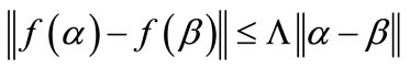 ,
, .
.
It is known that the Lipschitz constant is a “global” function’s feature that applies on the entirety of the domain that the function is defined. Especially for the time series, it is necessary to limit the influence of the Lipschitz constant in a subset of the domain of the function f by defining the local Lipschitz continuity. So, let Pi, where i = 1, 2, ···, n be the partition of the domain B on which function f is defined in [14].
Definition 3. Let Pi, i = 1, 2, ···, n be a subset of B; if function f is Lipschitz continuous on the open subset Pi, then the function is called local Lipschitz continuous in this subset.
In [3] was discussed the similarity between a time series and an objective function; based on this realization the usage of calculus tools—such as the local Lipschitz continuity—was extended to time series analysis, too.
2.2. The Usage of Local Lipschitz Constant Approximations as a Crisis Indicator
A different approach was discussed in [4] where it was proposed the application of an algorithm that enables the production of indicator-based alerts in order to obtain a crisis burst forecast. Although this algorithm is based on the “signal” extraction, it differentiates to such class of approaches on the nature of the indicator that is used.
Specifically, the indicator is approximated over a time series constructed from deductions of the local estimations of the Lipschitz constant, and results to the usage of the Lipschitz constant as the sole crisis indicator. The research of the local Lipschitz constant was motivated from previous realizations [3], where it was observed that a time series holds functional properties.
Recall that the Lipschitz constant is a function's constant that when is used in optimization it enables the acceleration of the optima search [15]; so the concept used in this study [3] was based on the measuring of a time series changes’ acceleration in means of changes that the values of the local Lipschitz-made series suffer.
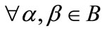
As already mentioned in [4,16] the proposed concept was that of comparing the last Lipschitz constant approximation Kt with the maximum one  resulting from all approximations on a subset {t – 1, t – 2, ···, t – m}.
Definition 4. A warning indicator A at point t raises when 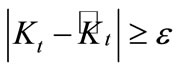 and it is symbolized by At = 1; note that ε is a determined level of significance [4].
Accordingly, the date that a crisis is possible to burst was considered as the trading day that corresponds to the last estimated t. Thus, an important characteristic of this methodology is that, although it provides forecasts prior to the burst, the prediction can be produced at the actual day of the burst.
2.3. The Future Interval Approach
The findings provided in [17] regarding the different convergence region according to the optimization technique used, motivated researching two techniques for the generation of an interval. The concept of the combinatory application of two techniques was further synthesized with the findings of [3] where the accommodation of time-oriented forecasts was succeeded based on the backtrack technique.
In specific, these methods focus on providing forecasts regarding the time that a time series will raise a future local, instead of the common practice of predicting the value at a next period. The logic behind these techniques is the mathematical approximation of the common characteristics amongst time series and real function that conclude on explaining the evolution phenomenon resting behind the series [18]. Additionally these methods are accompanied with convergence theorems that characterize the process of the approximation of the future local extremes.
However, a major drawback of the backtrack methods is that the estimated future point resulting from their application is not apparent whether it is the actual optimum or just a point that would eventually lead to an optimum. In fact it appears that the estimation of the future optimum is uncertain in means of suggesting a future point rather than a future interval.
In [5] this disadvantage is addressed by the generation of a interval that is eligible to enclose a time series future optima, by the usage of two different optimization methods. That methodological frame attempted to exploit two different backtrack forecasting methods towards entrapping the future optima by including it in the interval produced by the application of the dual-method. In fact, the double application produces a rather wide interval that is more vulnerable to enclose the future optimum since the two optimization techniques used have controversial convergence characteristics. Conclusively, the interval’s width tends to decrease as the time series approaches its critical value.
3. The Methodology towards Entrapping a Crisis
The revolutionary characteristic of this paper is the examination of an alerts-made time series in order to to entrap its optima. Simply, given a set of possible crisis dates we aim to envelop the crucial one in an interval that is created by applying two optimization techniques (on the initial set).
3.1. Stage A: Construction of the “Phantom” Time Series, Lt
On this stage is constructed the examined “phantom” time series Lt, which is defined as follows:
Definition 5. Let Lt be the “phantom” time series at t successive time intervals for which holds At = 1 and its values are the corresponding Kt.
In fact this time series is made of all the alerts producing when holds , and accordingly the value of each t component is the corresponding Kt (see Subsection 2.2 for calculation details).
3.2. Stage B: Estimation of the Cumulative Set
The second stage includes the backward search for the cumulative optimum set of points. Consider Lt as the “phantom” series of past approximations of the Lipschitz constant that have occurred from Stage A. Note that the time series is based on approximations of the Lipschitz constant, and thus let Lt be the “phantom” series corresponding to time intervals t = n, n – 1, n – 2, ···, n – m; set the backward stepsize equal to m. Note that this set will be a cumulative minimum one in case the past points follow an ascending stream and vice versa.
3.3. Stage C: Approaching of the Optimum Steplength
The optimum stepsize length Km is approached as the maximum local Lipschitz constant resulting from all feasible pairs of points that are included on the cumulative set of Stage B. Recall that the estimation of the local Lipschitz is succeeded as described in Definition 2.1.
3.4. Stage D: Approximation the Critical Interval
For the generation of the interval’s bound is exploited (a) the usage of the projection method as proposed by [19] and (b) estimations over the known Newton method. While application it was observed that as the methodology evolutes towards forecasting, the proposed interval’s lenght decreases given that it approaches the optimum; thus, the points resulting from the joint application of both methods eventually tend to agree.
Optimization Method A. For the assessment of the future extreme is used an appropriate steepest descent algorithm for unconstrained optimization [20]. The steplength is given from the Lipschitz constant approximation as follows:
 (2)
(2)
where wn is a case-determined stability coefficient.
Optimization Method B. The other bound is constructed based on estimations of the Newton method for unconstrained optimization. The required steplength m2 of the Newton method is given by the following relation,
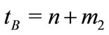 , (3)
, (3)
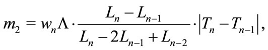 (4)
(4)
where wn is a heuristic stepsize magnifier.
The critical interval is (tL, tU) where tL and tU, are the lower and upper bounds, respectively. Consequently, for the boundary allocation of the method it holds, tL = min{tA, tB} and tU = max{tA, tB}. In [5] the convergence of that dual method application for any time series was proven.
A brief sketch of the proposed Entrapping Projection Algorithm is given in Algorithm 1.
4. Data and Obtained Results
The proposed methodology was applied on four time series originated from currency levels. Each series is constructed from observations over the trading year/s that a currency crisis burst, and assessed by the statistical package R [21].
Note that the methodology is applied on a regular basis regardless the date the crisis actually began. When application it was observed that the approximated intervals include the significant alerts, while their convergence was proved in [4]. Moreover, as the methodology evolutes towards approaching a forthcoming crisis period, more intervals regarding this critical period occur.
As mentioned the methodology is applied on series with daily and weekly data. The application on weekly data is also important because of the significant noise that characterizes the daily data. In the following figures it is apparent that, in the case of the weekly data series, the resulted intervals actually include the examined crises, and moreover their prediction was made three to four weeks prior to the critical date.
While application it was observed that experimenting on the length of the initial stepsize Λ is a matter of choice subject to each time series’ specifications; after all there is no such as a free lunch theorem. So for the estimation of the coefficient wn (for specification see Section 3) two alternatives are proposed based on the fitness
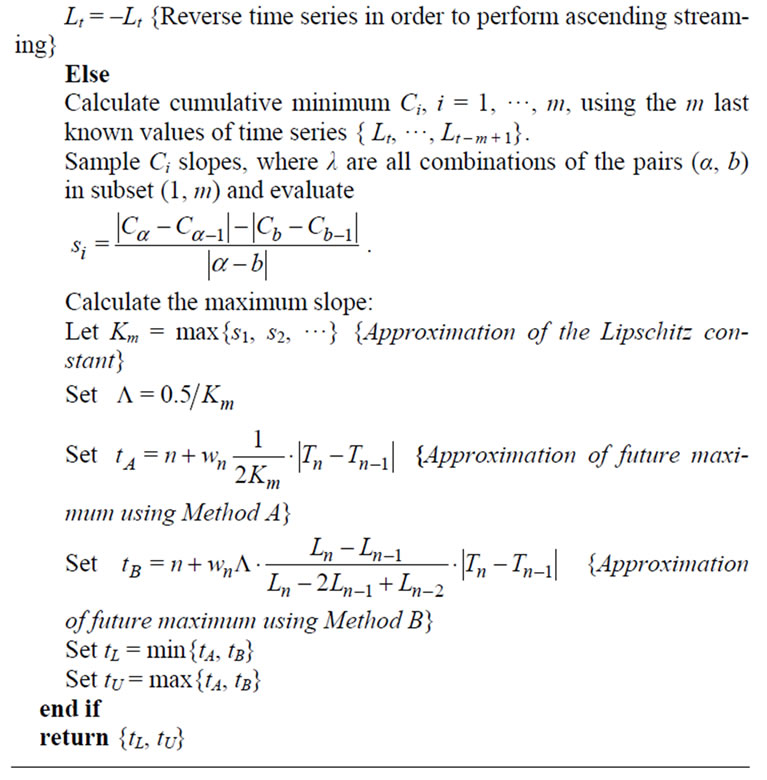
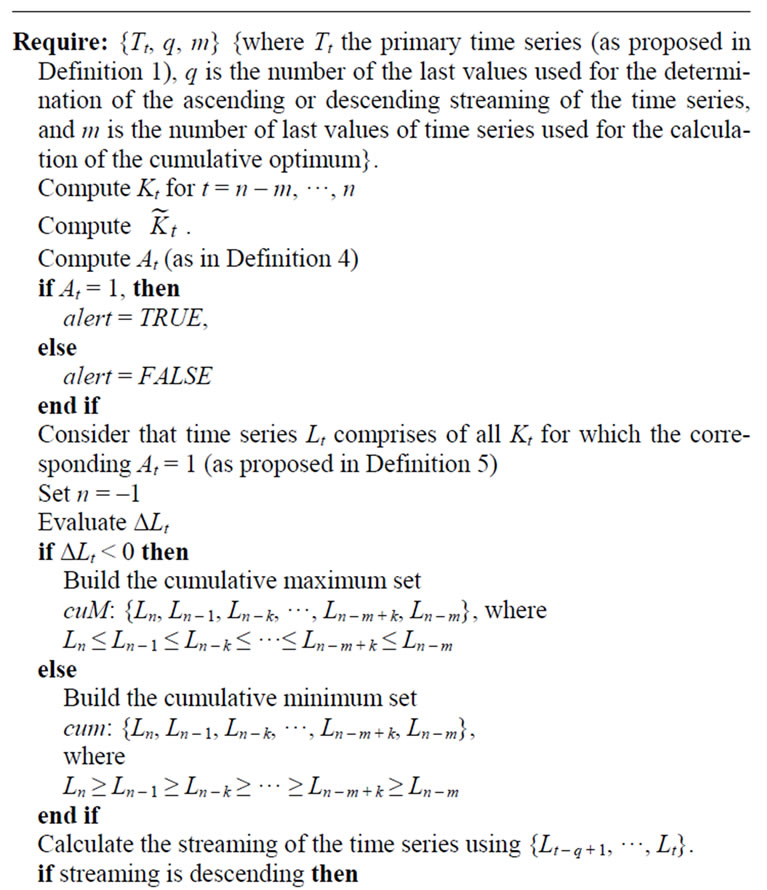
Algorithm 1. An outline of the Entrapping Projection Algorithm.
characteristics of the time series.
Thus this Section is organized as follows; Subsection 4.1 presents the results of time series with daily data, while the magnifier wn is estimated being equal to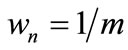 . In Subsection 4.2 that same approximation of the coefficient wn is applied on the time series comprising of weekly data. Finally in Subsection 4.3 the dailydata-made time series are accessed using a coefficient wn equal to
 .
.
The notation on each of the figures presenting on the following subsections is common and it is governed by four different features. The red bullets represent the possible alerts that raised by the application of the according methodology. The green bullets are used to signify the date that the proposed methodology predicted the oncoming crisis, while the actual crisis is shown by the blue bullet. The light red section of the figure demonstrates the whole period of the real crisis for the specific case.
4.1. Results Obtained Using Heuristic Magnifier ; Daily Data
4.1.1. The EURO Case
On Figure 1 the line assigns the daily Euro levels against the US dollar for the year from 11/11/2007 to 11/11/2008. Note that the Euro crisis bursted on 09/08/2008 and this date corresponds to the 273rd observation of the actual daily time series. Although the proposed methodology turned 19 critical intervals, only 5 of them include the critical date. However, for the assessment of the results the authors only consider those following a descent stream. This is due to the character of the search in question that is a crisis burst, so by default regards a rapid decrease of the value.
Accordingly, the 1st alert (it occurred on the 206th observation of the examined time series on date 03/06/2008, that is 206: 03/06/2010), the 4th (observation 253: 20/07/ 2008) and the 45th (on observation 269: 05/08/2008) are considered significantly important. As it occurs from Figure 1, the methodology came up with the first alert two months prior to the crisis burst-on the 03/06/2008. Note that the existence of an extensive upper bound of the interval reveals the long term character of the crisis.
4.1.2. The Mexican Peso Case
The tested time series is structured by the Mexican peso levels against the US dollar for a two-year period from January 1994 until the end of 1995, that is a dataset of 730 daily observations.
As seen on Figure 2 the methodology turned 21 possible critical intervals while two of them include the date of the actual crisis burst (355: 21/12/1994). The first of these two intervals was forecasted almost a month before the crisis burst; strangely, the second interval’s lower
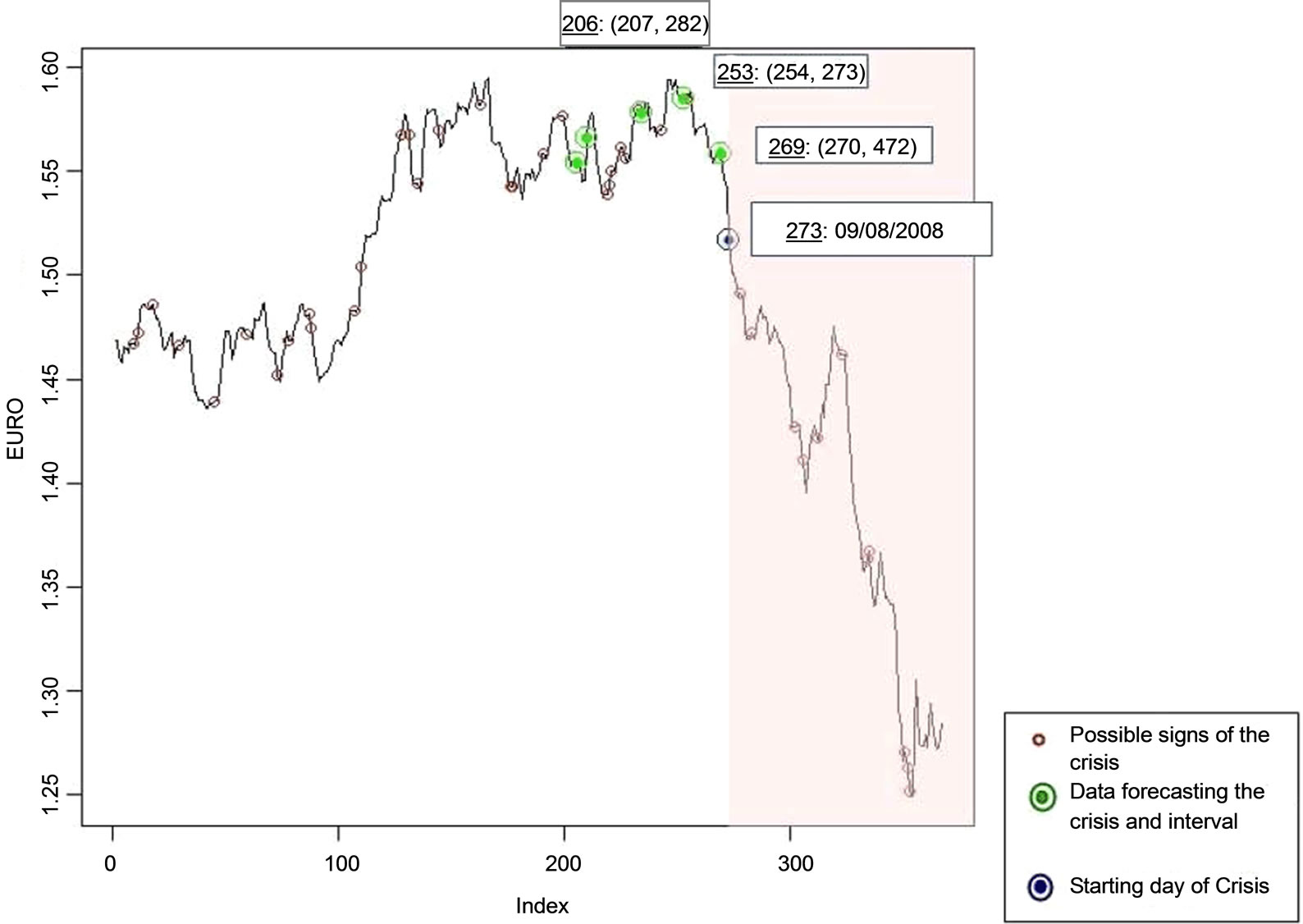
Figure 1. The critical features of the Euro daily levels against the US dollar for the period 11/11/2007-11/11/2008 using heuristic magnifier .
.
Figure 2. The critical features of the Mexican peso daily levels against the US dollar for the period 01/01/1994-31/12/1995 using heuristic magnifier .
.
bound is almost at the beginning of the crisis while the upper one coincides while the beginning of the temporarily smoothing period the series experienced. Moreover, the distance amongst the bounds declares the extensive character of the crisis.
4.1.3. The Russian Ruble Case
As seen on Figure 3, in this case the examined dataset includes the Russian ruble levels against the US dollar for the year 1998. The crisis date is the 237: 25/08/1998 and 4 of the 22 possible alerts predicted this date in their critical intervals. The earliest of the 4 successive intervals was predicted on 135: 15/05/1998, that is three months prior to the crisis burst. The majority of those intervals—3 out of 4—have a rather extensive upper bound and this feature is interpreted by the long descending stream of the currency levels.
4.1.4. The Turkish Lira Case
For this case (see Figure 4) the examined dataset covers a four-year period and it describes the daily observations of the Turkish lira levels against the US dollar for the period 02/01/2000-31/12/2004.
In the daily series case, the application of the methodology resulted on a lone interval that does not include the actual starting date of the crisis. A possible explanation would be the rapid descending stream of the examined time series.
4.2. Results Obtained Using Heuristic Magnifier ; Weekly Data
While application it was observed that the usage of weekly observations provides rather stable results since it is free of noise that probably affects the daily data.
4.2.1. The EURO Case
On Figure 5 it is apparent that the critical week, that is the 40th one, was predicted by the methodology 3 weeks before the crisis bursted. Also in this case, 1 out of the 7 total turned intervals included the critical date.
4.2.2. The Mexican Peso Case
Alike the previous EURO case, on this case the methodology turned one successful interval (see Figure 6). Moreover, the effective prediction was made three weeks
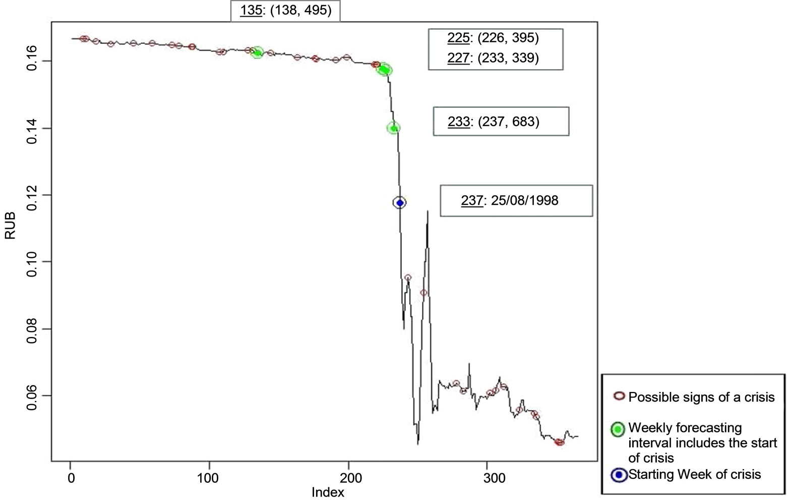
Figure 3. The critical features of the Russian ruble daily levels against the US dollar for the period 01/01/1998-31/12/1998 using heuristic magnifier .
.
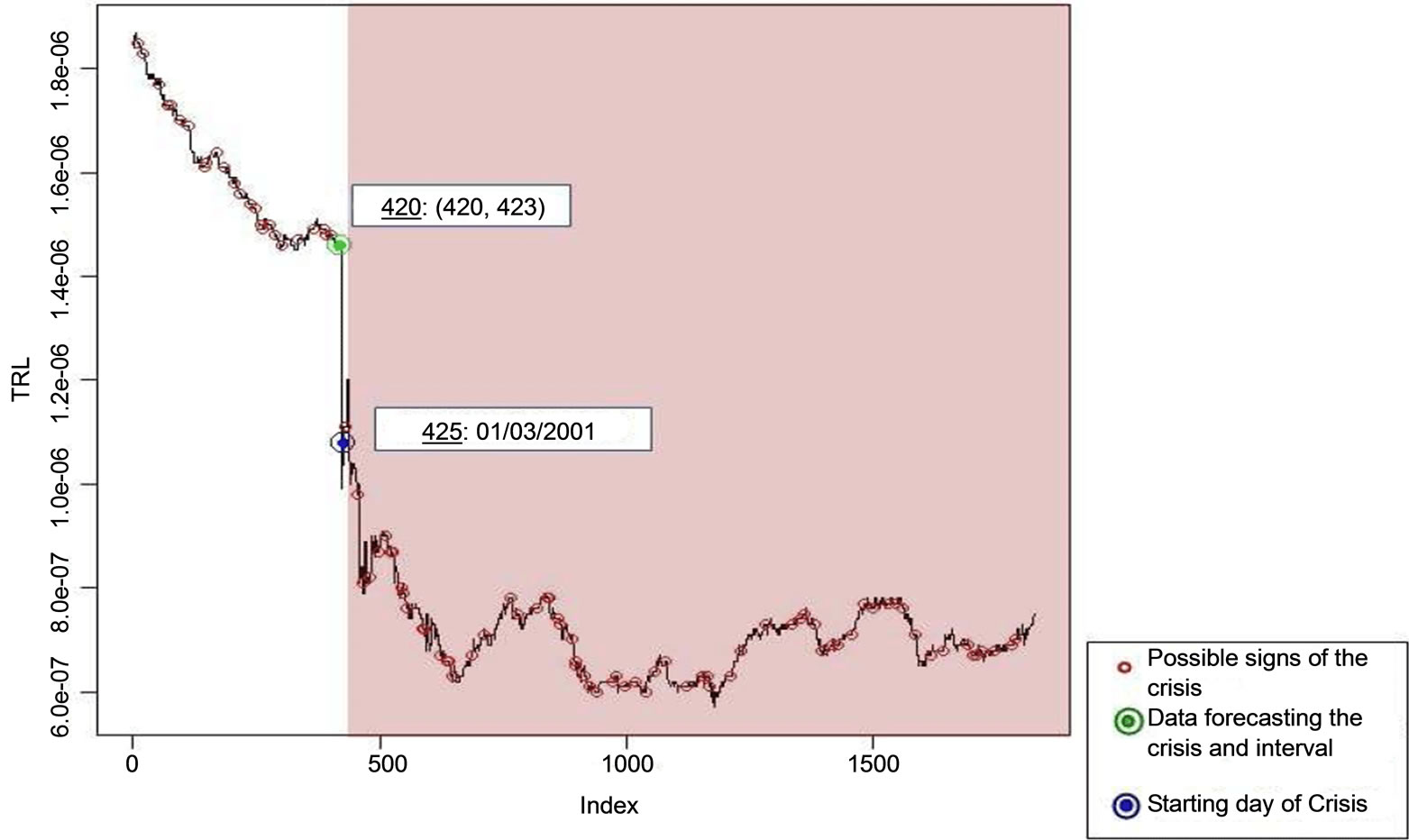
Figure 4. The critical features of the Turkish lira daily levels against the US dollar for the period 02/01/2000-31/12/2004 using heuristic magnifier .
.
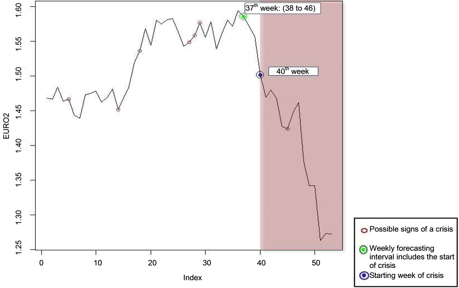
Figure 5. The critical features of the Euro weekly levels against the US dollar for the period 11/11/2007-11/11/2008 using heuristic magnifier .
.
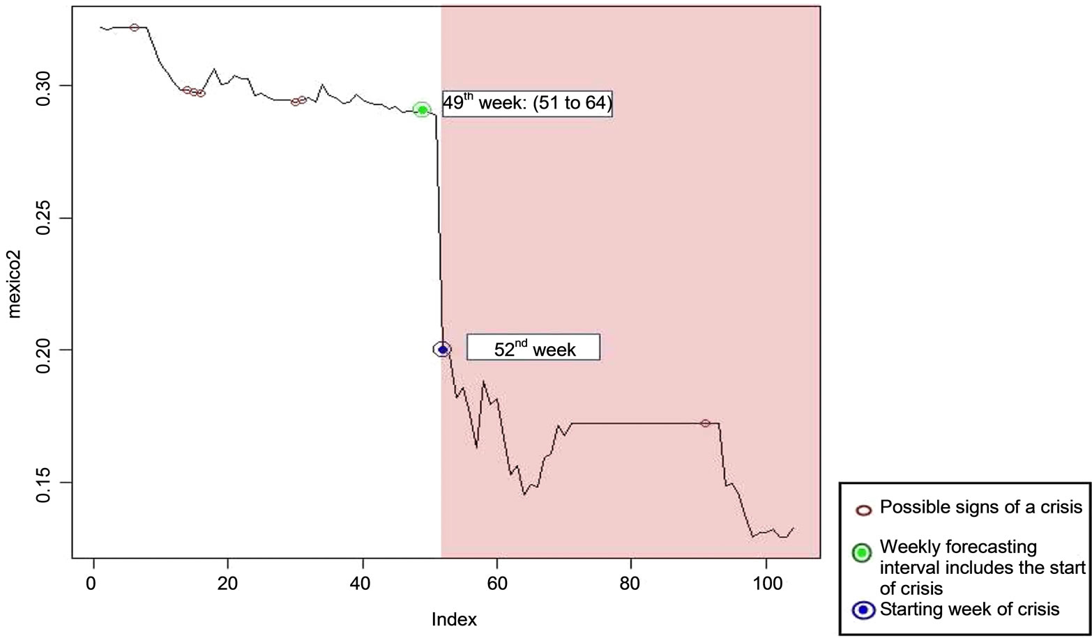
Figure 6. The critical features of the Mexican peso weekly levels against the US dollar for the period 01/01/1994-31/12/1995 using heuristic magnifier .
.
before the crisis burst. As it appears from Figure 6 the upper bound of the interval coincides with the smooth part of the time series that follows the crisis period.
4.2.3. The Russian Ruble Case
On Figure 7 it is obvious that the crisis began on the 34th week of the examined period; this period was predicted by the methodology 4 weeks prior to the crisis occurrence. Alike the majority of most results, the upper bound of the interval coincides with the week right before the steep descent that followed the crisis period.
4.2.4. The Turkish Lira Case
On Figure 8, it appears that the prediction regarding the 51st week should be rejected because the time series at that point follows an ascending stream. Thus the interval that regards the 59th week, is the one that includes the critical week when the crisis in Turkey bursted.
At last, Table 1 represents an outline of the critical intervals obtained from the application of the heuristic magnifier  on daily and weekly data. On this table the column labeled “Case” displays the crisis case that is examined, while the second column shows the examined period for the specific case. On the column named “Burst date” is assigned the actual date that the crisis burst was recorded. Finally, the fourth and fifth columns are assigned by the number of daily and weekly observations, that comprise the examined series.
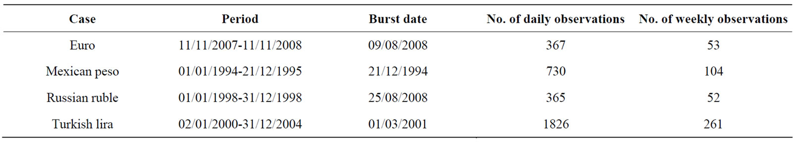
Table 1. Summary of output critical intervals.
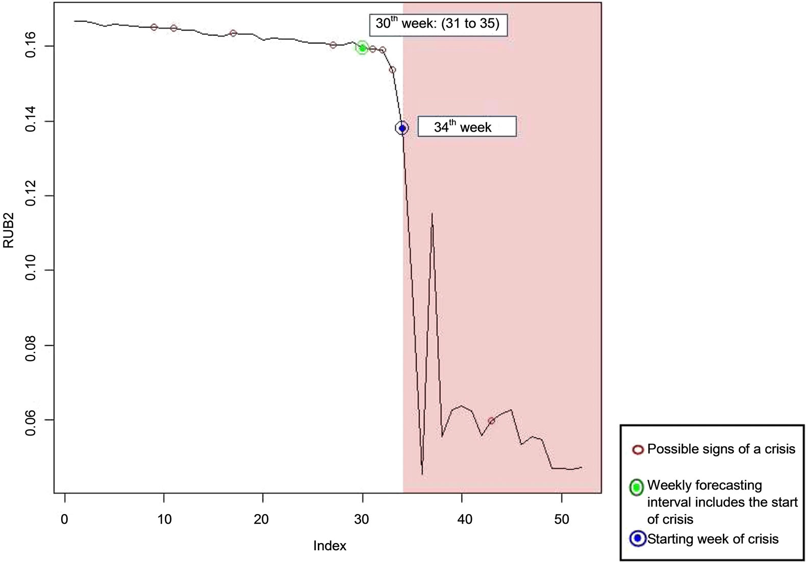
Figure 7. The critical features of the Russian ruble weekly levels against the US dollar for the period 01/01/1998-31/12/1998 using heuristic magnifier .
.
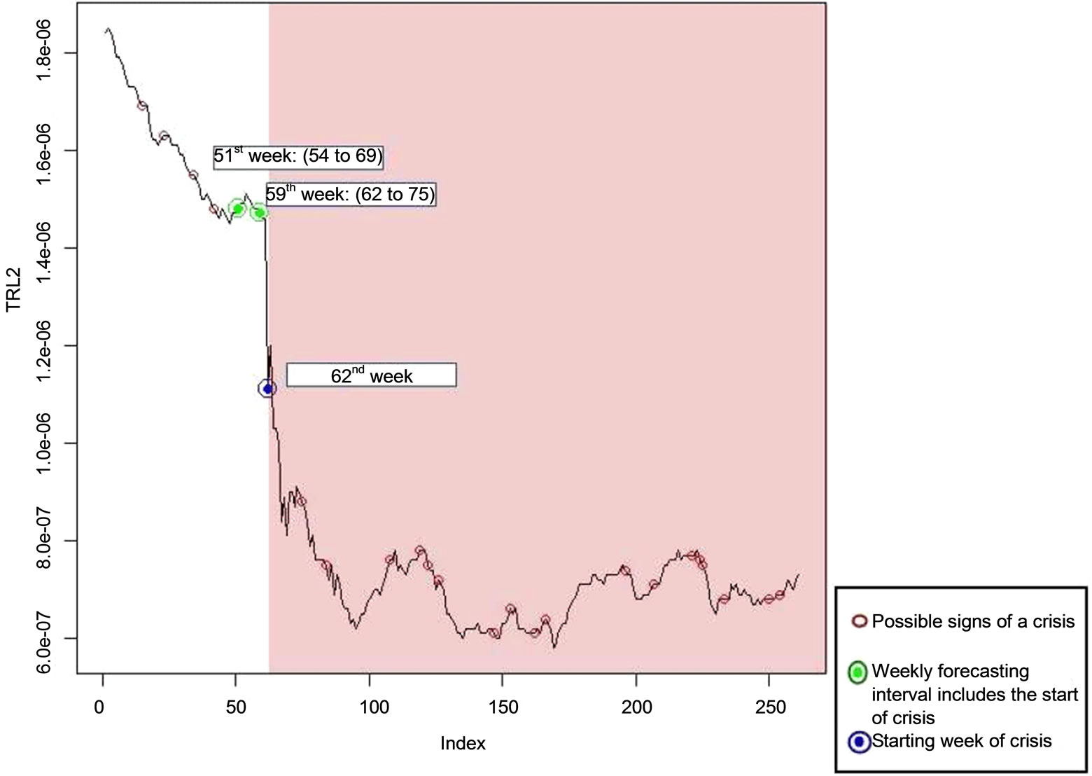
Figure 8. The critical features of the Turkish lira weekly levels against the US dollar for the period 02/01/2000-31/12/2004 using heuristic magnifier .
.
4.3. Results Obtained Using Heuristic Magnifier ; Daily Data
4.3.1. The EURO Case
As provided on Figure 9 the predicted interval resulted using a heuristic magnifier wn equal to  for the period of time describing in Table 1. Recall that the examined time series comprises by the Euro daily levels against the US dollar for the period 11/11/2007- 11/11/2008.
Alike the results in Subsection 4.1, the Entrapping Projection Algorithm (Alg.) turned 19 alerts. However, the crucial differentiation amongst the results that obtained from both methods, is that the usage of the heuristic magnifier equal to  provides much earlier predictions. For i.e. in this case, the prediction regarding the crisis date (273: 09/08/2008) occurred three months before its burst, at observation-date 163: 21/04/ 1998.
4.3.2. The Mexican Peso Case
Similarly to the observations made on Figure 9, the intervals produced based on the Mexican peso daily levels against the US dollar for the period 01/01/1994-31/12/ 1995, are earlier than those observed using the other heuristic magnifier (Subsection 4.1).
On the associated Figure 10, it worth noting the observation 329: 25/11/1994. On that date both techniques predicted intervals that include the starting day of a crisis, regardless the fact that these intervals are different. Moreover, in this case it is also observed that the upper bounds of the 2—out of 3 total—intervals mark the critical period.
Finally, although the number of possible alerts remains the same (as in the case that  holds), the number of the critical intervals is lower; in fact there are 3 intervals. Additionally, the interval’s upper bound coincides with the temporary smoothness of the series and probably define the interval’s crisis.
4.3.3. The Russian Ruble Case
Figure 11 represents the critical values when examined the Russian ruble daily levels against the US dollar for the period 01/01/1998-31/12/1998 using a stepsize magnifier . Although in both previous cases the application of the
  stepsize magnifier provided earlier intervals, as seen on Figure 11 this
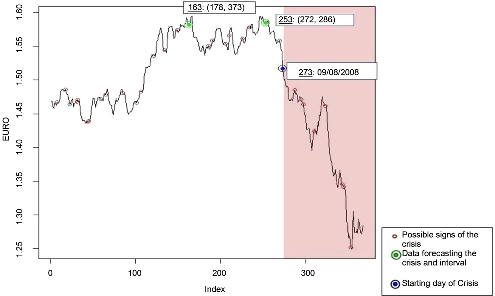
Figure 9. The critical features of the Euro daily levels against the US dollar for the period 11/11/2007-11/11/2008 using heuristic magnifier .
.
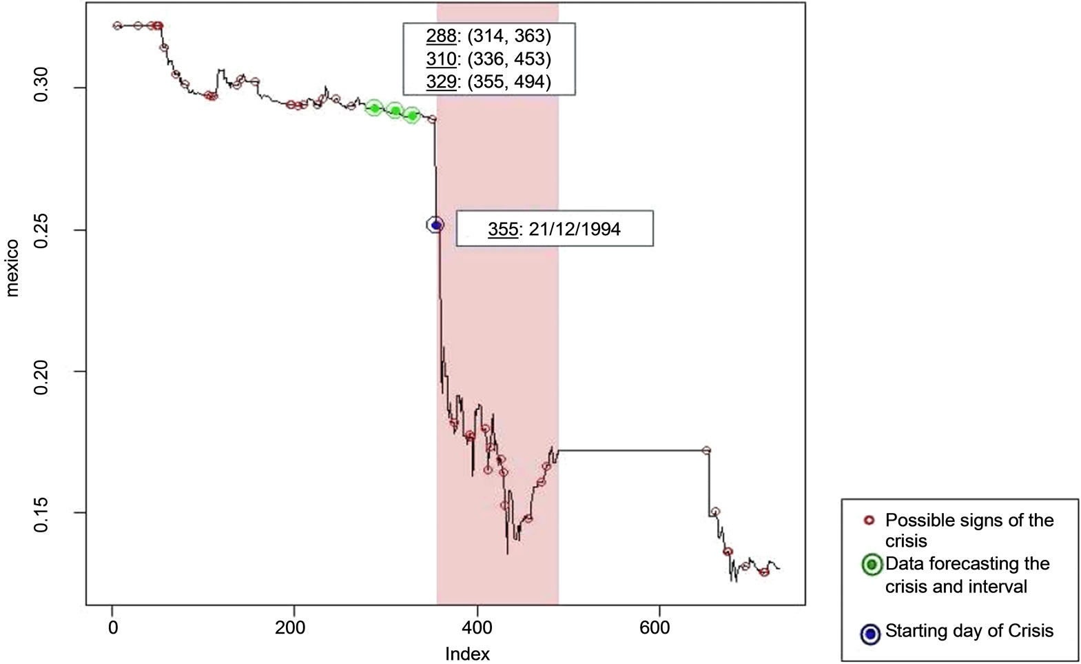
Figure 10. The critical features of the Mexican peso daily levels against the US dollar for the period 01/01/1994-31/12/1995 using heuristic magnifier .
.
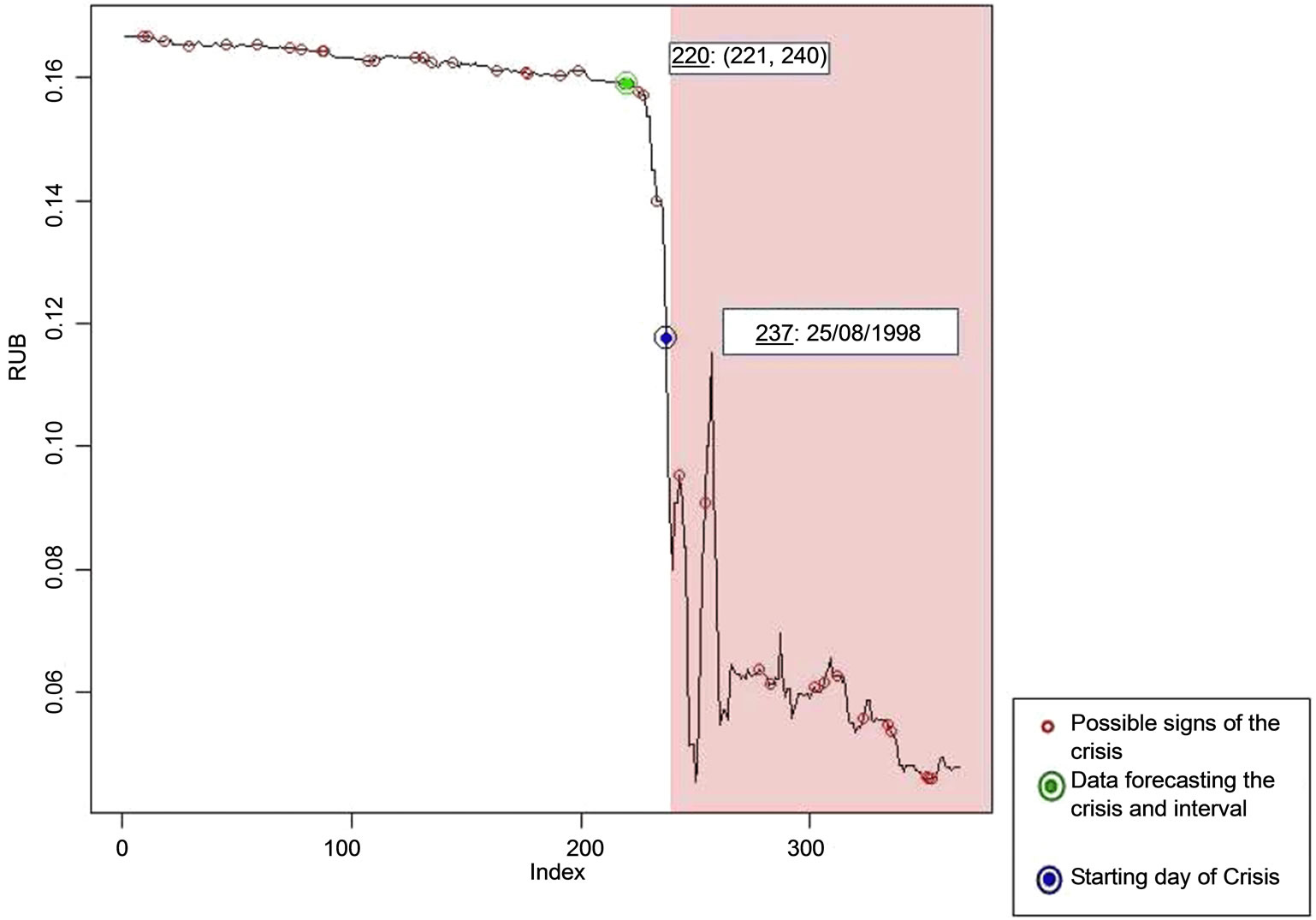
Figure 11. The critical features of the Russian ruble daily levels against the US dollar for the period 01/01/1998-31/12/1998 using heuristic magnifier .
.
time the resulted interval was a latter one; i.e. in this case the prediction of the crisis was made 17 days before its burst, in contrast to the other case of calculation that the successful prediction was made 135 days before the burst.
4.3.4. The Turkish Lira Case
In this case the data set includes the Turkish lira daily levels against the US dollar for the period 02/01/ 2000-31/12/2004 and the approximation of the predictions is made using a stepsize magnifier  (Figure 12).
As it occurs the crisis burst (observation-date 425: 01/03/2001) was predicted on 3 intervals; while the very first successful prediction was made on the 364th observation, that is 61 days prior to the crisis date. Also note that the upper bound of the intervals on the 364th and the 386th observations coincide with the two major descents of the time series’ values.
In general, in the case of daily data the choice of the appropriate heuristic stepsize magnifier wn is subject to its suitability to the data examined. As far as it concerns the type of data—daily or weekly—the usage of the weekly data results to earlier and more efficient prediction; this is an observation that empowers the “ex-ante” character of the methodology as an Early Warning System.
5. Findings and Discussion
With this paper is attempted to incorporate with the major issue of detecting future critical intervals of time that are eligible to enclose a financial crisis burst. The convergence of the conjoint application of two techniques on the same dataset and with the same initial point has proved in [5] and the ability of the Lipschitz constant estimation to indicate a crisis burst has also proved in [4].
The suggested methodology was tested on four time series comprising of currency levels and the examined data covered periods of major financial crises. The time series were examined under three different spectrums; firstly was used daily and weekly information and secondly an alternative heuristic stepsize magnifier was applied for the daily panel.
The weekly results produced—in the majority of the cases—earlier and more efficient predictions regarding the crisis ahead. Specifically the predictions, most of the times, were made almost three months before the examined crisis did actually burst. The daily results also oper-
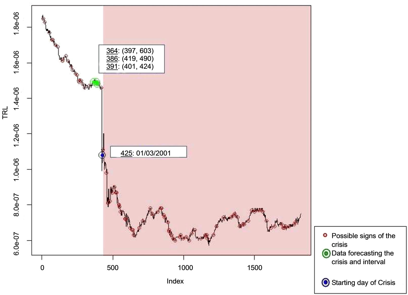
Figure 12. The critical features of the Turkish lira daily levels against the US dollar for the period 02/01/2000-31/12/2004 using heuristic magnifier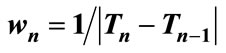 .
.
ated efficiently, however the forecasts were not as “early” as those provided when the weekly data panel was used. Moreover, the usage of two different heuristic stepsize magnifiers for the process of the daily time series proved that the application of that magnifier is subject to the data's nature and not a dogma that governs all cases.
The findings and observations of this study are rather promising since the application resulted to an efficient “ex-ante” prediction of the crisis ahead, and this fact reveals the methodology’s Early Warning ability.
The proposed analysis may be also applied in other research areas where the monetary limitations of the money market cease to exist. Also the examination of other optimization techniques that study the generation of intervals might include previous points by applying a further step. Probable extension of the proposed interval framework may be researched on the generation of a strategic tool that would enhance the portfolio optimization process. Moreover, in the case of the portfolio’s trade, it possible for the attractive intervals to coincide-inbetween equitiesand hence gain from the minimization of the transaction costs required; and this is a good way to maximize the net returns. In the same direction, the exploitation of the lexicographic optimization features may also advance the usage of optimum intervals when optimizing portfolio.
REFERENCES
- G. Kaminsky, S. Lizondo and C. M. Reinhart, “Leading Indicators of Currency Crises,” International Monetary Fund Staff Papers, Vol. 1, No. 1, 1998, pp. 1-48. doi:10.2307/3867328
- A. Berg and C. Pattillo, “Predicting Currency Crises: The Indicators Approach and an Alternative,” Journal of International Money and Finance, Vol. 18, No. 4, 1999, pp. 561-586. doi:10.1016/S0261-5606(99)00024-8
- E. G. Lisgara and G. S. Androulakis, “Estimating Time Series Future Optima Using a Steepest Descent Methodology as a Backtracker,” Proceedings of the International Multiconference on Computer Science and Information Technology, Wisla, 20-22 October 2008, pp. 893- 898.
- G. S. Androulakis and E. G. Lisgara, “Exploiting the Usage of the Lipschitz Constant Approximations as a Financial Crisis Indicator,” submitted, 2011.
- E. G. Lisgara, G. I. Karolidis, and G. S. Androulakis, “Entrapping a Time Series Future Optima Using a Combination of Optimization Techniques,” Proceedings of the 24 Mini EURO Conference on Continuous Optimization and Information-Based Technologies in The Financial Sector, Izmir, 23-26 June 2010, pp. 24-29.
- G. Kaminsky and C. M. Reinhart, “The Twin Crises: The causes of Banking and Balance-of-Payments Problems,” American Economic Review, Vol. 89, No. 3, 1999, pp. 473- 500. doi:10.1257/aer.89.3.473
- R. Majhi, G. Panda and G. Sahoo, “Efficient prediction of Exchange Rates with Low Complexity Artificial Neural Network Models,” Expert Systems with Applications, Vol. 36, No. 1, 2009, pp. 181-189. doi:10.1016/j.eswa.2007.09.005
- R. Dornbusch, I. Goldfajn and R. O. Valdes, “Currency Crises and Collapses,” Brookings Papers on Economic Activity, Vol. 26, No. 2, 1995, pp. 219-294. doi:10.2307/2534613
- P. Krugman, “Are Currency Crises Self-Fulfilling?” NBER Macroeconomics Annual, Vol. 11, 1996, pp. 345-407. doi:10.2307/3585207
- V. Coudert and M. Gex, “Does Risk Aversion Drive Financial Crises? Testing the Predictive Power of Empirical Indicators,” Journal of Empirical Finance, Vol. 15, No. 2, 2007, pp. 167-184. doi:10.1016/j.jempfin.2007.06.001
- M. Bussiere and M. Fratzscher, “Towards a New Early Warning System of Financial Crises,” Journal of International Money and Finance, Vol. 25, No. 6, 2006, pp. 953- 973. doi:10.1016/j.jimonfin.2006.07.007
- A. Berg and R. E. Coke, “Autocorrelation-Corrected Standard Errors in Panel Probits: An Application to CurRency Crisis Prediction,” Technical Report: International Monetary Fund, 2004.
- J. Berg, B. Candelon and J. Urbain, “A Cautious Note on the Use of Panel Models to Predict Financial Crises,” Economics Letters, Vol. 101, No. 2, 2008, pp. 80-83. doi:10.1016/j.econlet.2008.06.015
- M. Abramowitz and I. A. Stegun, “Handbook of Mathematical Functions with Formulas, Graphs, and Mathematical Tables,” National Bureau of Standards Applied Mathematics, 1997.
- A. Molinaro, C. Pizzuti and Y. D. Sergeyev, “Acceleration Tools for Diagonal Information Global Optimization Algorithms,” Computational Optimization and Applications, Vol. 18, No. 1, 2001, pp. 5-26. doi:10.1023/A:1008719926680
- E. G. Lisgara, G. I. Karolidis and G. S. Androulakis, “A Progression of the Backtrack Optimization Technique Forforecasting Potential Financial Crisisperiods,” Proceedings of the Conference in Numerical Analysis, Recent Approaches to Numerical Analysis: Theory, Methods and Applications, 15-18 September 2010, pp. 126-133.
- G. S. Androulakis and M. N. Vrahatis, “OPTAC: A Portable Software Package for Analyzing and Comparing Optimization Methods by Visualization,” Journal of Computational and Applied Mathematics, Vol. 72, No. 1, 1996, pp. 41-62. doi:10.1016/0377-0427(95)00244-8
- G. S. Androulakis, “A Technique for Entrapping a Time Series Future Optima,” Proceedings of the Conference in Numerical Analysis, Recent Approaches to Numerical Analysis: Theory, Methods and Applications, 15-18 September 2010, pp. 19-23.
- G. I. Karolidis, E. G. Lisgara and G. S. Androulakis, “A New Projection Method for Predicting Time Series Points,” Proceedings of the 24 Mini EURO Conference on Continuous Optimization and Information Based Technologies in The Financial Sector, Izmir, 23-26 June 2010, pp. 18-23.
- G. S. Androulakisand and E. G. Lisgara, “On the Prediction of Time Series’ Local Optima: A Backtrack Technique,” Proceedings of the Conference in Numerical Analysis, Recent Approaches to Numerical Analysis: Theory, Methods and Applications, Kalamata, 3-7 September 2007, pp. 19-23.
- R Development Core Team, “R: A Language and Environment for Statistical Computing,” R Foundation for Statistical Computing, Vienna, 2008. http://www.R-project.org