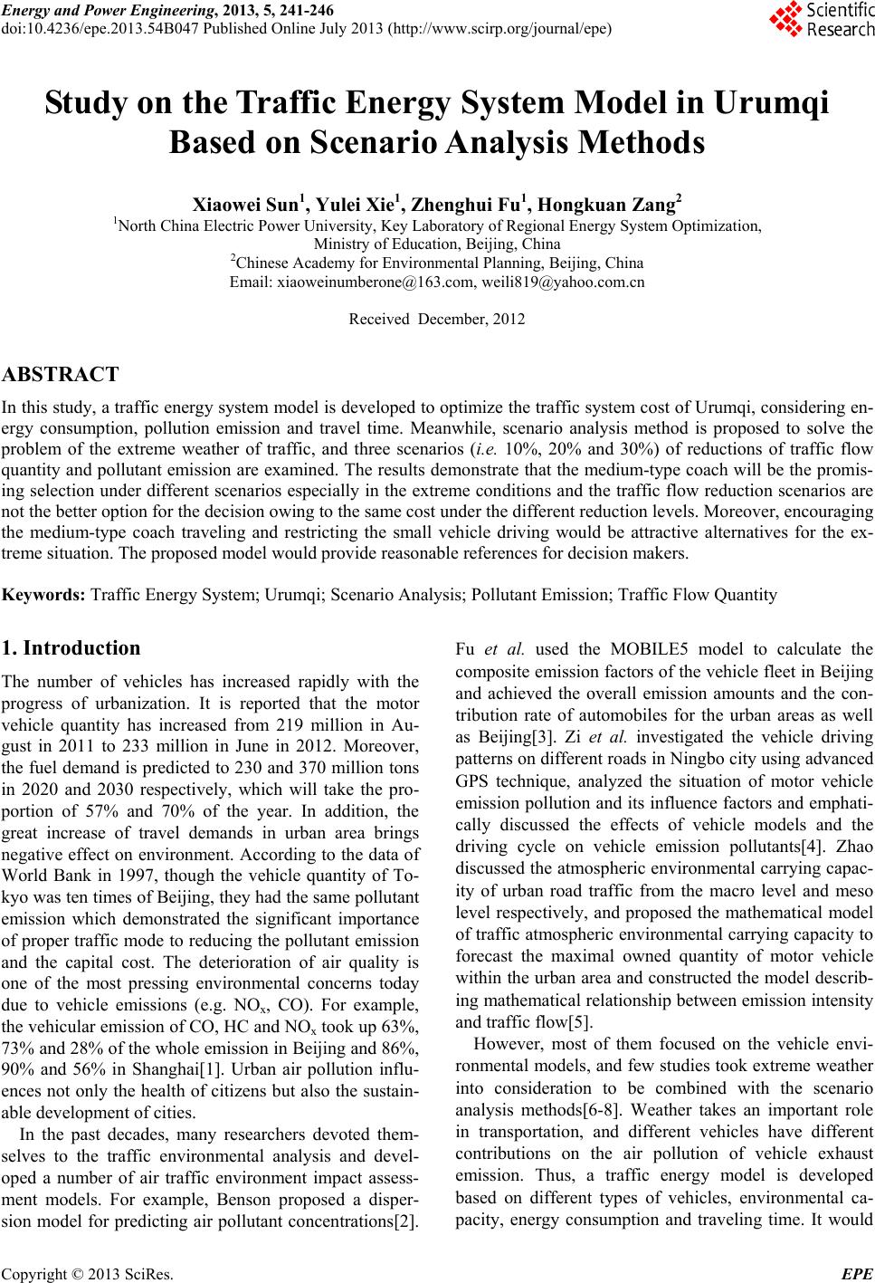
Energy and Power Engineering, 2013, 5, 241-246
doi:10.4236/epe.2013.54B047 Published Online July 2013 (http://www.scirp.org/journal/epe)
Study on the Traffic Energy System Model in Urumqi
Based on Scenario Analysis Methods
Xiaowei Sun1, Yulei Xie1, Zhenghui Fu1, Hongkuan Zang2
1North China Electric Power University, Key Laboratory of Regional Energy System Optimization,
Ministry of Education, Beijing, China
2Chinese Academy for Environmental Planning, Beijing, China
Received December, 2012
ABSTRACT
In this study, a traffic energy system model is developed to optimize the traffic system cost of Urumqi, considering en-
ergy consumption, pollution emission and travel time. Meanwhile, scenario analysis method is proposed to solve the
problem of the extreme weather of traffic, and three scenarios (i.e. 10%, 20% and 30%) of reductions of traffic flow
quantity and pollutant emission are examined. The results demonstrate that the medium-type coach will be the promis-
ing selection under different scenarios especially in the extreme conditions and the traffic flow reduction scenarios are
not the better option for the decision owing to the same cost under the different reduction levels. Moreover, encouraging
the medium-type coach traveling and restricting the small vehicle driving would be attractive alternatives for the ex-
treme situation. The proposed model would provide reasonable references for decision makers.
Keywords: Traffic Energy System; Urumqi; Scenario Analysis; Pollutant Emission; Traffic Flow Quantity
1. Introduction
The number of vehicles has increased rapidly with the
progress of urbanization. It is reported that the motor
vehicle quantity has increased from 219 million in Au-
gust in 2011 to 233 million in June in 2012. Moreover,
the fuel demand is predicted to 230 and 370 million tons
in 2020 and 2030 respectively, which will take the pro-
portion of 57% and 70% of the year. In addition, the
great increase of travel demands in urban area brings
negative effect on environment. According to the data of
World Bank in 1997, though the vehicle quantity of To-
kyo was ten times of Beijing, they had the same pollutant
emission which demonstrated the significant importance
of proper traffic mode to reducing the pollutant emission
and the capital cost. The deterioration of air quality is
one of the most pressing environmental concerns today
due to vehicle emissions (e.g. NOx, CO). For example,
the vehicular emission of CO, HC and NOx took up 63%,
73% and 28% of the whole emission in Beijing and 86%,
90% and 56% in Shanghai[1]. Urban air pollution influ-
ences not only the health of citizens but also the sustain-
able development of cities.
In the past decades, many researchers devoted them-
selves to the traffic environmental analysis and devel-
oped a number of air traffic environment impact assess-
ment models. For example, Benson proposed a disper-
sion model for predicting air pollutant concentrations[2].
Fu et al. used the MOBILE5 model to calculate the
composite emission factors of the vehicle fleet in Beijing
and achieved the overall emission amounts and the con-
tribution rate of automobiles for the urban areas as well
as Beijing[3]. Zi et al. investigated the vehicle driving
patterns on different roads in Ningbo city using advanced
GPS technique, analyzed the situation of motor vehicle
emission pollution and its influence factors and emphati-
cally discussed the effects of vehicle models and the
driving cycle on vehicle emission pollutants[4]. Zhao
discussed the atmospheric environmental carrying capac-
ity of urban road traffic from the macro level and meso
level respectively, and proposed the mathematical model
of traffic atmospheric environmental carrying capacity to
forecast the maximal owned quantity of motor vehicle
within the urban area and constructed the model describ-
ing mathematical relationship between emission intensity
and traffic flow[5].
However, most of them focused on the vehicle envi-
ronmental models, and few studies took extreme weather
into consideration to be combined with the scenario
analysis methods[6-8]. Weather takes an important role
in transportation, and different vehicles have different
contributions on the air pollution of vehicle exhaust
emission. Thus, a traffic energy model is developed
based on different types of vehicles, environmental ca-
pacity, energy consumption and traveling time. It would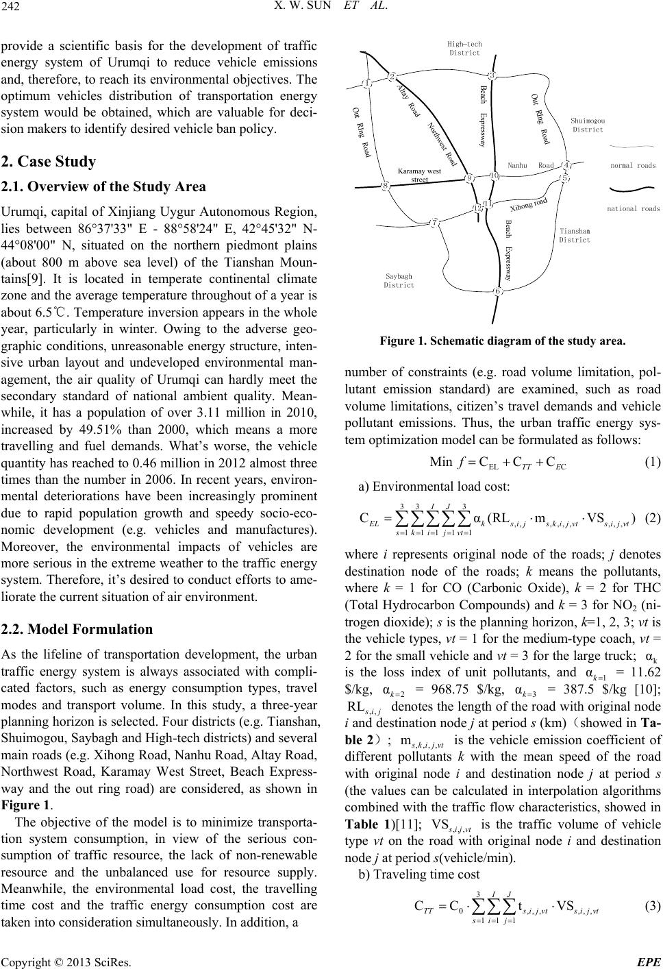

X. W. SUN ET AL.
242
provide a scientific basis for the development of traffic
energy system of Urumqi to reduce vehicle emissions
and, therefore, to reach its environmental objectives. The
optimum vehicles distribution of transportation energy
system would be obtained, which are valuable for deci-
sion makers to identify desired vehicle ban policy.
2. Case Study
2.1. Overview of the Study Area
Urumqi, capital of Xinjiang Uygur Autonomous Region,
lies between 86°37'33" E - 88°58'24" E, 42°45'32" N-
44°08'00" N, situated on the northern piedmont plains
(about 800 m above sea level) of the Tianshan Moun-
tains[9]. It is located in temperate continental climate
zone and the average temperature throughout of a year is
about 6.5℃. Temperature inversion appears in the whole
year, particularly in winter. Owing to the adverse geo-
graphic conditions, unreasonable energy structure, inten-
sive urban layout and undeveloped environmental man-
agement, the air quality of Urumqi can hardly meet the
secondary standard of national ambient quality. Mean-
while, it has a population of over 3.11 million in 2010,
increased by 49.51% than 2000, which means a more
travelling and fuel demands. What’s worse, the vehicle
quantity has reached to 0.46 million in 2012 almost three
times than the number in 2006. In recent years, environ-
mental deteriorations have been increasingly prominent
due to rapid population growth and speedy socio-eco-
nomic development (e.g. vehicles and manufactures).
Moreover, the environmental impacts of vehicles are
more serious in the extreme weather to the traffic energy
system. Therefore, it’s desired to conduct efforts to ame-
liorate the current situation of air environment.
2.2. Model Formulation
As the lifeline of transportation development, the urban
traffic energy system is always associated with compli-
cated factors, such as energy consumption types, travel
modes and transport volume. In this study, a three-year
planning horizon is selected. Four districts (e.g. Tianshan,
Shuimogou, Saybagh and High-tech districts) and several
main roads (e.g. Xihong Road, Nanhu Road, Altay Road,
Northwest Road, Karamay West Street, Beach Express-
way and the out ring road) are considered, as shown in
Figure 1.
The objective of the model is to minimize transporta-
tion system consumption, in view of the serious con-
sumption of traffic resource, the lack of non-renewable
resource and the unbalanced use for resource supply.
Meanwhile, the environmental load cost, the travelling
time cost and the traffic energy consumption cost are
taken into consideration simultaneously. In addition, a
Figure 1. Schematic diagram of the study ar ea.
number of constraints (e.g. road volume limitation, pol-
lutant emission standard) are examined, such as road
volume limitations, citizen’s travel demands and vehicle
pollutant emissions. Thus, the urban traffic energy sys-
tem optimization model can be formulated as follows:
EL C
Min CCC
TT E
f

 (1)
a) Environmental load cost:
33 3
,,, ,, ,,, ,
1111 1
Cα(RL mVS)
IJ
E
Lksijskijvt
ski jvt 

 sijvt
 (2)
where i represents original node of the roads; j denotes
destination node of the roads; k means the pollutants,
where k = 1 for CO (Carbonic Oxide), k = 2 for THC
(Total Hydrocarbon Compounds) and k = 3 for NO2 (ni-
trogen dioxide); s is the planning horizon, k=1, 2, 3; vt is
the vehicle types, vt = 1 for the medium-type coach, vt =
2 for the small vehicle and vt = 3 for the large truck; k
is the loss index of unit pollutants, and 1
α
αk

= 11.62
$/kg, 2 αk

= 968.75 $/kg, 3 αk = 387.5 $/kg [10];
,,
RL
s
ij
m
denotes the length of the road with original node
i and destination node j at period s (k m)（showed in Ta-
ble 2）; ,,,,
s
kijvt is the vehicle emission coefficient of
different pollutants k with the mean speed of the road
with original node i and destination node j at period s
(the values can be calculated in interpolation algorithms
combined with the traffic flow characteristics, showed in
Table 1)[11]; ,,, VS
s
ijvt is the traffic volume of vehicle
type vt on the road with original node i and destination
node j at period s(vehicle/min).
b) Traveling time cost
3
0,,,
11 1
CCt VS
IJ
TTs ij vts ij vt
si j  
 
 ,,,
(3)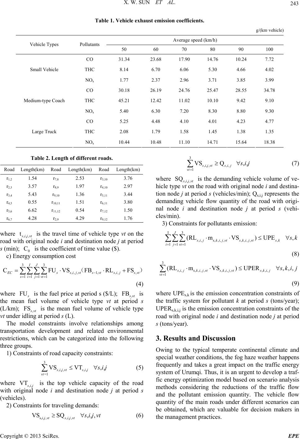

X. W. SUN ET AL.
243
Table 1. Vehicle exhaust emission coefficients.
g/(km·vehicle)
Average speed (km/h)
Vehicle Types Pollutants
50 60 70 80 90 100
CO 31.34 23.68 17.90 14.76 10.24 7.72
THC 8.14 6.70 6.06 5.30 4.66 4.02
Small Vehicle
NOx 1.77 2.37 2.96 3.71 3.85 3.99
CO 30.18 26.19 24.76 25.47 28.55 34.78
THC 45.21 12.42 11.02 10.10 9.42 9.10
Medium-type Coach
NOx 5.40 6.30 7.20 8.30 8.80 9.30
CO 5.25 4.48 4.10 4.01 4.23 4.77
THC 2.08 1.79 1.58 1.45 1.38 1.35 Large Truck
NOx 10.44 10.48 11.10 14.71 15.64 18.38
Table 2. Length of different roads. 3
,,, ,,
1
VSQ, ,
sijvtsi j
vt
s
ij


 (7)
Road Length(km) Road Length(km) Road Length(km)
r1,2 1.54 r7,8 2.53 r3,10 3.76
r2,3 3.57 r8,9 1.97 r4,10 2.97
r3,4 5.43 r9,10 1.36 r5,11 3.44
r4,5 0.55 r10,11 1.51 r6,11 3.80
r5,6 6.62 r11,12 0.54 r7,12 1.50
r6,7 4.28 r2,9 4.29 r9,12 1.76
where ,,,
SQ
s
ijvt is the demanding vehicle volume of ve-
hicle type vt on the road with original node i and destina-
tion node j at period s (vehicles/min); Qs,i,j represents the
demanding vehicle flow quantity of the road with origi-
nal node i and destination node j at period s (vehi-
cles/min).
3) Constraints for pollutants emission:
where ,,,
t
s
ijvt
C
is the travel time of vehicle type vt on the
road with original node i and destination node j at period
s (min); is the coefficient of time value ($).
I3
,,s, ,, ,, ,, ,,
111
(RLmVS) UPE,
J
s ijk ij vts k ij vts k
ijvt
s
k

 

0
c) Energy consumption cost (8)
33
,, ,1,,,,
11 11
CFUVSFBRL
IJ
FS
E
Cssi jvtsvtsi jsvt
si jvt  

 （）
(4)
3
,,s, ,, ,, ,, ,, ,,
1
(RLmVS)UPER,, ,
sij kijvtskijvtskij
vt
s
kij

 

(9)
where UPEs,k is the emission concentration constraints of
the traffic system for pollutant k at period s (tons/year);
UPERs,k,i,j is the emission concentration constraints of the
road with original node i and destination node j at period
s (tons/year).
where FU
s
is the fuel price at period s ($/L); , FB
s
vt is
the mean fuel volume of vehicle type vt at period s
(L/km); , FS
s
vt is the mean fuel volume of vehicle type
vt under idling at period s (L).
The model constraints involve relationships among
transportation development and related environmental
restrictions, which can be categorized into the following
three groups.
3. Results and Discussion
Owing to the typical temperate continental climate and
special weather conditions, the fog haze weather happens
frequently and takes a great impact on the traffic energy
system of Urumqi. Thus, it is an urgent to develop a traf-
fic energy optimization model based on scenario analysis
methods considering the reductions of the traffic flow
and the pollutant emission quantity. The vehicle flow
quantity of the main roads under different scenarios can
be obtained, which are valuable for decision makers in
the management practices.
1) Constraints of road capacity constraints:
3
,,, ,,
=1
VSVT, ,
sijvt sij
vt
s
ij
 (5)
where ,, VT
s
ij is the top vehicle capacity of the road
with original node i and destination node j at period s
(vehicles).
2) Constraints for traveling demands:
s, , ,, , ,
VSSQ,, ,
ijvt sijvt
s
ijvt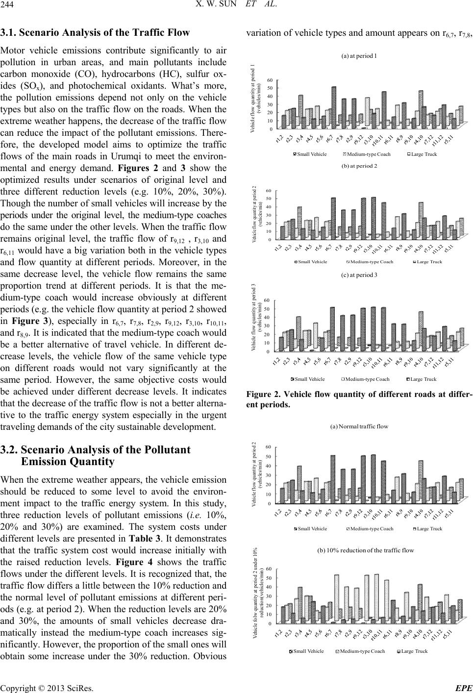 (6)

X. W. SUN ET AL.
244
3.1. Scenario Analysis of the Traffic Flow
Motor vehicle emissions contribute significantly to air
pollution in urban areas, and main pollutants include
carbon monoxide (CO), hydrocarbons (HC), sulfur ox-
ides (SOx), and photochemical oxidants. What’s more,
the pollution emissions depend not only on the vehicle
types but also on the traffic flow on the roads. When the
extreme weather happens, the decrease of the traffic flow
can reduce the impact of the pollutant emissions. There-
fore, the developed model aims to optimize the traffic
flows of the main roads in Urumqi to meet the environ-
mental and energy demand. Figures 2 and 3 show the
optimized results under scenarios of original level and
three different reduction levels (e.g. 10%, 20%, 30%).
Though the number of small vehicles will increase by the
periods under the original level, the medium-type coaches
do the same under the other levels. When the traffic flow
remains original level, the traffic flow of r9,12 , r3,10 and
r6,11 would have a big variation both in the vehicle types
and flow quantity at different periods. Moreover, in the
same decrease level, the vehicle flow remains the same
proportion trend at different periods. It is that the me-
dium-type coach would increase obviously at different
periods (e.g. the vehicle flow quantity at period 2 showed
in Figure 3), especially in r6,7, r7,8, r2,9, r9,12, r3,10, r10,11,
and r8,9. It is indicated that the medium-type coach would
be a better alternative of travel vehicle. In different de-
crease levels, the vehicle flow of the same vehicle type
on different roads would not vary significantly at the
same period. However, the same objective costs would
be achieved under different decrease levels. It indicates
that the decrease of the traffic flow is not a better alterna-
tive to the traffic energy system especially in the urgent
traveling demands of the city sustainable development.
3.2. Scenario Analysis of the Pollutant
Emission Quantity
When the extreme weather appears, the vehicle emission
should be reduced to some level to avoid the environ-
ment impact to the traffic energy system. In this study,
three reduction levels of pollutant emissions (i.e. 10%,
20% and 30%) are examined. The system costs under
different levels are presented in Table 3. It demonstrates
that the traffic system cost would increase initially with
the raised reduction levels. Figure 4 shows the traffic
flows under the different levels. It is recognized that, the
traffic flow differs a little between the 10% reduction and
the normal level of pollutant emissions at different peri-
ods (e.g. at period 2). When the reduction levels are 20%
and 30%, the amounts of small vehicles decrease dra-
matically instead the medium-type coach increases sig-
nificantly. However, the proportion of the small ones will
obtain some increase under the 30% reduction. Obvious
variation of vehicle types and amount appears on r6,7, r7,8,
0
10
20
30
40
50
60
Vehicle flow quantity at period 1
(vehicles/min)
(a) at period 1
Small VehicleMedium-type CoachLarge Truck
0
10
20
30
40
50
60
Vehicle flow quantity at period 2
(vehicles/min)
(b) at period 2
Small VehicleMedium-type CoachLarge Truck
0
10
20
30
40
50
60
Vehicle flow quantity at period 3
(vehicles/min)
(c) at period 3
Small VehicleMedium-type CoachLarge Truck
Figure 2. Vehicle flow quantity of different roads at differ-
ent periods.
0
10
20
30
40
50
60
Vehicle flow quantity at period 2
(vehicles/min)
(a) Normal traffic flow
Small VehicleMedium-type CoachLarge Truck
0
10
20
30
40
50
60
Vehicle folw quantity at period 2 under 10%
reduction(vehicles/min)
(b) 10% reduction of the traffic flow
Small VehicleMedium-type CoachLarge Truck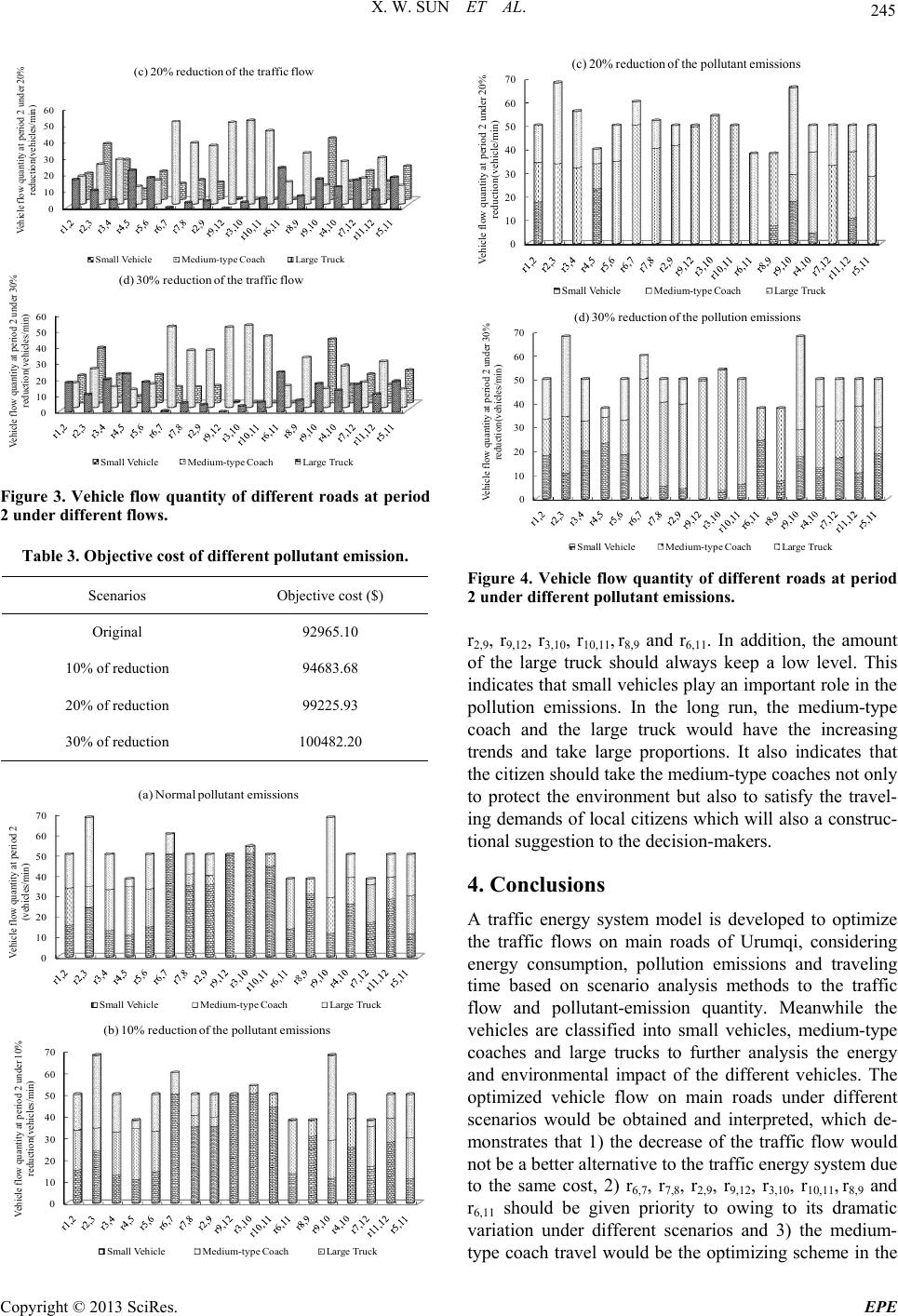

X. W. SUN ET AL. 245
0
10
20
30
40
50
60
Vehicle flow quantity at period 2 under 20%
reduction(vehicles/min)
(c) 20% reduction of the traffic flow
Small VehicleMedium-type CoachLarge Truck
0
10
20
30
40
50
60
Vehicle flow quantity at period 2 under 30%
reduction(vehicles/min)
(d) 30% reduction of the traffic flow
Small VehicleMedium-type CoachLarge Truck
Figure 3. Vehicle flow quantity of different roads at period
2 under different flows.
Table 3. Objective cost of different pollutant emission.
Scenarios Objective cost ($)
Original 92965.10
10% of reduction 94683.68
20% of reduction 99225.93
30% of reduction 100482.20
0
10
20
30
40
50
60
70
Vehicle flow quantity at period 2
(veh i cles/mi n )
(a) Normal pollutant emissions
Small VehicleMedium-type CoachLarge Truck
0
10
20
30
40
50
60
70
Vehicle flow quantity at period 2 under 10%
reduction(vehicles/min)
(b) 10% reduction of the pollutant emissions
Small VehicleMedium-type CoachLarge Truck
0
10
20
30
40
50
60
70
Vehicle flow quantity at period 2 under 20%
reduction(vehicle/min)
(c) 20% reduction of the pollutant emissions
Small VehicleMedium-type CoachLarge Truck
0
10
20
30
40
50
60
70
Vehicle flow quantity at period 2 under 30%
red uctio n(vehicl es /min)
(d) 30% reduction of the pollution emissions
Small VehicleMedium-type CoachLarge Truck
Figure 4. Vehicle flow quantity of different roads at period
2 under different pollutant emissions.
r2,9, r9,12, r3,10, r10,11, r8,9 and r6,11. In addition, the amount
of the large truck should always keep a low level. This
indicates that small vehicles play an important role in the
pollution emissions. In the long run, the medium-type
coach and the large truck would have the increasing
trends and take large proportions. It also indicates that
the citizen should take the medium-type coaches not only
to protect the environment but also to satisfy the travel-
ing demands of local citizens which will also a construc-
tional suggestion to the decision-makers.
4. Conclusions
A traffic energy system model is developed to optimize
the traffic flows on main roads of Urumqi, considering
energy consumption, pollution emissions and traveling
time based on scenario analysis methods to the traffic
flow and pollutant-emission quantity. Meanwhile the
vehicles are classified into small vehicles, medium-type
coaches and large trucks to further analysis the energy
and environmental impact of the different vehicles. The
optimized vehicle flow on main roads under different
scenarios would be obtained and interpreted, which de-
monstrates that 1) the decrease of the traffic flow would
not be a better alternative to the traffic energy system due
to the same cost, 2) r6,7, r7,8, r2,9, r9,12, r3,10, r10,11, r8,9 and
r6,11 should be given priority to owing to its dramatic
variation under different scenarios and 3) the medium-
type coach travel would be the optimizing scheme in the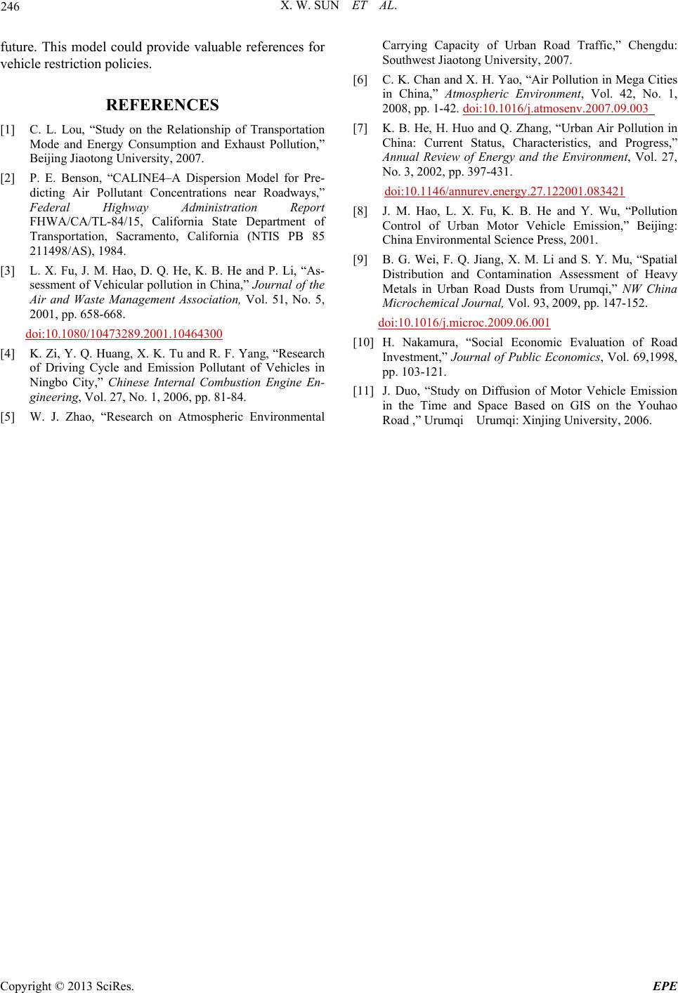

X. W. SUN ET AL.
246
future. This model could provide valuable references for
vehicle restriction policies.
REFERENCES
[1] C. L. Lou, “Study on the Relationship of Transportation
Mode and Energy Consumption and Exhaust Pollution,”
Beijing Jiaotong University, 2007.
[2] P. E. Benson, “CALINE4–A Dispersion Model for Pre-
dicting Air Pollutant Concentrations near Roadways,”
Federal Highway Administration Report
FHWA/CA/TL-84/15, California State Department of
Transportation, Sacramento, California (NTIS PB 85
211498/AS), 1984.
[3] L. X. Fu, J. M. Hao, D. Q. He, K. B. He and P. Li, “As-
sessment of Vehicular pollution in China,” Journal of the
Air and Waste Management Association, Vol. 51, No. 5,
2001, pp. 658-668.
doi:10.1080/10473289.2001.10464300
[4] K. Zi, Y. Q. Huang, X. K. Tu and R. F. Yang, “Research
of Driving Cycle and Emission Pollutant of Vehicles in
Ningbo City,” Chinese Internal Combustion Engine En-
gineering, Vol. 27, No. 1, 2006, pp. 81-84.
[5] W. J. Zhao, “Research on Atmospheric Environmental
Carrying Capacity of Urban Road Traffic,” Chengdu:
Southwest Jiaotong University, 2007.
[6] C. K. Chan and X. H. Yao, “Air Pollution in Mega Cities
in China,” Atmospheric Environment, Vol. 42, No. 1,
2008, pp. 1-42. doi:10.1016/j.atmosenv.2007.09.003
[7] K. B. He, H. Huo and Q. Zhang, “Urban Air Pollution in
China: Current Status, Characteristics, and Progress,”
Annual Review of Energy and the Environment, Vol. 27,
No. 3, 2002, pp. 397-431.
doi:10.1146/annurev.energy.27.122001.083421
[8] J. M. Hao, L. X. Fu, K. B. He and Y. Wu, “Pollution
Control of Urban Motor Vehicle Emission,” Beijing:
China Environmental Science Press, 2001.
[9] B. G. Wei, F. Q. Jiang, X. M. Li and S. Y. Mu, “Spatial
Distribution and Contamination Assessment of Heavy
Metals in Urban Road Dusts from Urumqi,” NW China
Microchemical Journal, Vol. 93, 2009, pp. 147-152.
doi:10.1016/j.microc.2009.06.001
[10] H. Nakamura, “Social Economic Evaluation of Road
Investment,” Journal of Public Economics, Vol. 69,1998,
pp. 103-121.
[11] J. Duo, “Study on Diffusion of Motor Vehicle Emission
in the Time and Space Based on GIS on the Youhao
Road ,” Urumqi Urumqi: Xinjing University, 2006.