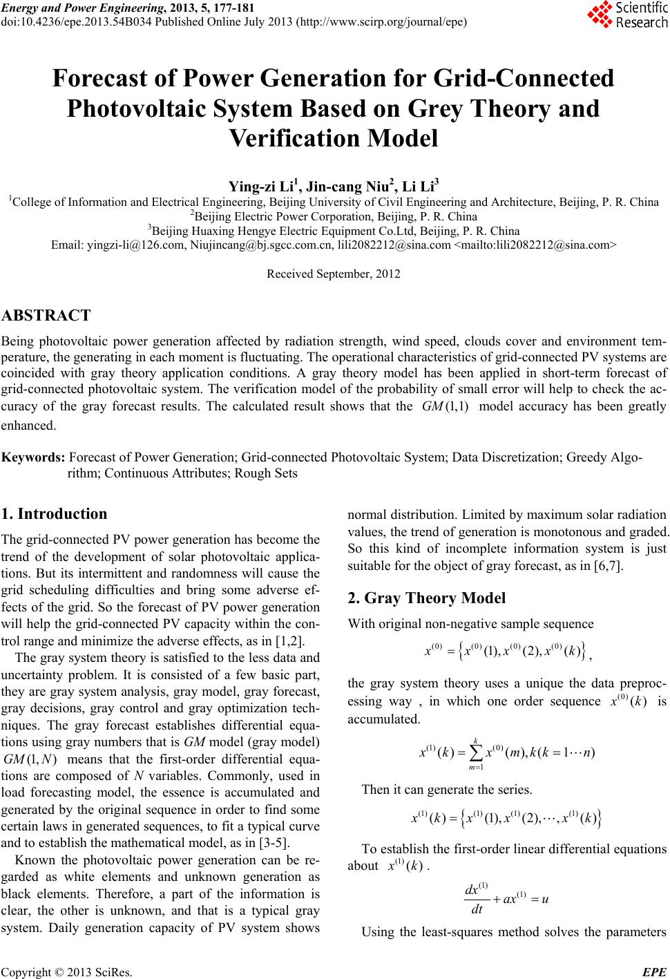Energy and Power Engineering, 2013, 5, 177-181
doi:10.4236/epe.2013.54B034 Published Online July 2013 (http://www.scirp.org/journal/epe)
Forecast of Power Generation for Grid-Connected
Photovoltaic System Based on Grey Theory and
Verification Model
Ying-zi Li1, Jin-cang Niu2, Li Li3
1College of Information and Electrical Engineering, Beijing University of Civil Engineering and Architecture, Beijing, P. R. China
2Beijing Electric Power Corporation, Beijing, P. R. China
3Beijing Huaxing Hengye Electric Equipment Co.Ltd, Beijing, P. R. China
Received September, 2012
ABSTRACT
Being photovoltaic power generation affected by radiation strength, wind speed, clouds cover and environment tem-
perature, the generating in each moment is fluctuating . The operational characteristics of grid-connected PV systems are
coincided with gray theory application conditions. A gray theory model has been applied in short-term forecast of
grid-connected photovoltaic system. The verification model of the probability of small error will help to check the ac-
curacy of the gray forecast results. The calculated result shows that th1) model accuracy has been greatly
enhanced
e
.
(1,GM
Keywords: Forecast of Power Generation; Grid-connected Photovoltaic System ; Data Discretization; Greedy Algo-
rithm; Continuous Attributes; Rough Sets
1. Introduction
The grid-connected PV power generation has become the
trend of the development of solar photovoltaic applica-
tions. But its intermittent and randomness will cause the
grid scheduling difficulties and bring some adverse ef-
fects of the grid. So the forecast of PV power generation
will help the grid-connected PV capacity within the con-
trol range and minimize the adverse effects, as in [1,2].
The gray system theory is satisfied to th e less data and
uncertainty problem. It is consisted of a few basic part,
they are gray system analysis, gray model, gray forecast,
gray decisions, gray control and gray optimization tech-
niques. The gray forecast establishes differential equa-
tions using gray numbers that is GM model (gray model)
means that the first-order differential equa-
tions are composed of N variables. Commonly, used in
load forecasting model, the essence is accumulated and
generated by the original sequence in order to find some
certain laws in generated sequen ces, to fit a typical curve
and to establish th e mathematical model, as in [3-5].
(1, )GM N
Known the photovoltaic power generation can be re-
garded as white elements and unknown generation as
black elements. Therefore, a part of the information is
clear, the other is unknown, and that is a typical gray
system. Daily generation capacity of PV system shows
normal distribution. Limited by maximum solar radiation
values, the trend of generation is monotonous and graded.
So this kind of incomplete information system is just
suitable for the object of gray forecast, as in [6,7].
2. Gray Theory Model
With original non- negati ve sa mple sequence


(0)(0) (0)(0)
(1), (2), ()
x
xx xk,
the gray system theory uses a unique the data preproc-
essing way , in which one order sequence (0) ()
x
k is
accumulated.
(1) (0)
1
()( ),(1)
k
m
x
kxmkk


n
Then it can generate the series.


(1)(1) (1)(1)
()(1), (2),, ()
x
kx xxk
To establish the first-order linear differential equations
about (1) ()
x
k.
(1) (1)
dx ax u
dt


Using the least-squares method solves the parameters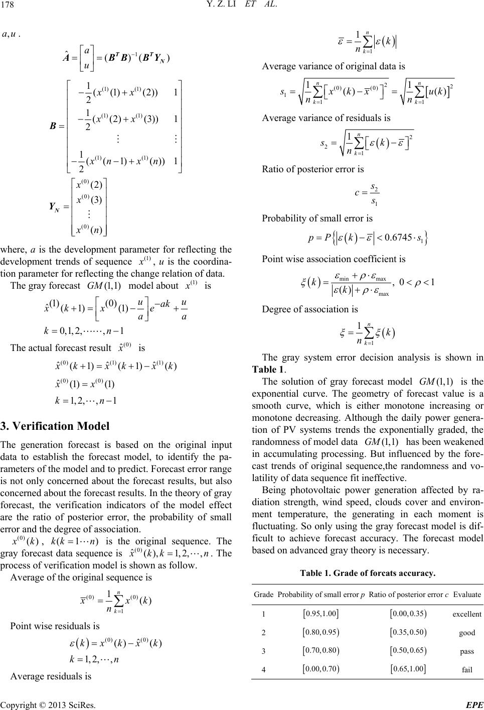

Y. Z. LI ET AL.
178
,au.
1
ˆ()(
a
u





TT
N
ABBB )Y
(1) (1)
(1) (1)
(1) (1)
(0)
(0)
(0)
1((1)(2)) 1
2
1( (2)(3))1
2
1((1) ())1
2
(2)
(3)
()
xx
xx
xn xn
x
x
xn




















N
B
Y






where, a is the development parameter for reflecting the
development trends of sequence (1)
x
, u is the coordina-
tion parameter for r e f l e c t i ng the change rel a tion of da ta.
The gray forecast model about
(1,1)GM (1)
x
is
(1) (0)
ˆ(1)(1)
0,1,2,, 1
uu
ak
xk xe
aa
kn


 



The actual forecast result (0)
ˆ
x
is
(0)(1) (1)
(0) (0)
ˆˆˆ (1)(1) (
ˆ(1) (1)
1, 2,,1
)
x
kxkx
xx
kn
 


k
3. Verification Model
The generation forecast is based on the original input
data to establish the forecast model, to identify the pa-
rameters of the model and to predict. Forecast error range
is not only concerned about the forecast results, but also
concerned about the forecast results. In the theory of gray
forecast, the verification indicators of the model effect
are the ratio of posterior error, the probability of small
error and the degree of association.
(0) ()
x
k, is the original sequence. The
gray forecast data sequence is
(1kk n)(0)
ˆ(),1,2, ,
x
kk n. The
process of verification model is shown as follow.
Average of th e original sequence is
(0) (0)
1
1()
n
k
x
xk
n

Point wise residuals is

(0) (0)
ˆ () ()
1, 2,,
kxkxk
kn
 

Averag e residuals is

1
1n
k
k
n



Average variance of original data is

22
(0) (0)
111
11
() ()
nn
kk
s
xkx uk
nn





Average variance of residuals is

2
21
1n
k
sk
n






Ratio of posterior error is
2
1
s
c
s

Probability of small error is



1
0.6745pP ks 


Point wise association coefficient is

min max
max
, 01
()
kk







Degree of association is

1
1n
k
k
n



The gray system error decision analysis is shown in
Table 1.
The solution of gray forecast model is the
exponential curve. The geometry of forecast value is a
smooth curve, which is either monotone increasing or
monotone decreasing. Although the daily power genera-
tion of PV systems trends the exponentially graded, the
randomness of model data has been we aken ed
in accumulating processing. But influenced by the fore-
cast trends of original sequence,the randomness and vo-
latility of data sequence fit ineffective.
(1,1)GM
(1,1)GM
Being photovoltaic power generation affected by ra-
diation strength, wind speed, clouds cover and environ-
ment temperature, the generating in each moment is
fluctuating. So only using the gray forecast model is dif-
ficult to achieve forecast accuracy. The forecast model
based on advanced gray theory is necessary.
Table 1. Grade of forcats accuracy.
GradeProbability of small error pRatio of posterior error cEvaluate
1


0.95,1.00

 0.00,0.35 excellent
2


0.80,0.95
 
0.35,0.50 good
3


0.70,0.80


0.50,0.65 pass
4


0.00,0.70


0.65,1.00 fail

Y. Z. LI ET AL. 179
Forecast steps of advanced gray model are
given as follow. (1,1)GM
Firstly, it is calculated relative deviation between the
forecast value (0)
ˆ()
x
k and actual value (0)()
x
k during
the former moment n.
(0) (0)
(0)
ˆ
() ()
(),1,2, ,
()
xkxk
kk
xk

 n
Secondly, above relative error will be divided into i
states., expressed as 12 ,,,
i
s
ss
12
12min max
[, ],1,2
,[(),()
iii
ii
si
kk]




 

If (0) (0)(0)
ˆˆˆ
(1),(2), ,()
x
nxn xnk

1,( 2),nn
k is the gray
forecast value at moment ,( )n

.
(0) (0)
12
12
(0) (0)
ˆˆ () ()
,
ˆˆ
() ()
1, 2,,1,,
ii
ii
x
xnx xn
xn xn
innnk






12
,
ii
x
x is the gray forecast range. According to the
biggest relative deviation state probability and the gray
forecast range


12
,
ii
x
x, gray forecast results can be
modified to increase the forecast accuracy.
4. Calculation Example
The actual operation data of one day is used as example
in this paper, which is 15 minutes interval.
With photovoltaic generating presented synchroniza-
tion trends with th e sun radiation, two models
are established respectively applying the data from 8:00
to 12:00 and 12:00 to 15:00.
(1,1)GM
The original non-negative sample sequence form 8:00
to 11:15 is (0)
1
x
(0)
1{0.2305,0.3197,0.3308,0.3714,0.4443,
0.4868,0.5383,0.5310,0.6025,0.6528,
0.6828,0.7055,0.6704,0.7140}
x

The original non-negative sample sequence form 12:
15 to 14:15 is (0)
2
x
(0)
2{0.7338,0.7333,0.7079,0.6938,0.6463,
0.5901,0.5518,0.5358,0.4840}
x
The sequences of acculturational data is
(1)
1
(1)
2
{0.2305,0.5502,0.8810,1.2524,1.6966,
2.1833,2.7216,3.2526,3.8551,4.5079,
5.1906,5.8961,6.5665,7.2805}
{0.7338,1.4670,2.1749,2.8687,3.5149,
4.1050,4.6567,5.1925
x
x


,5.6765}
Using the least-squares method to solve parameters
, there are ,au
11
11111
1
21
22222
2
-0.0 630
ˆ()( )
0.3374
0.0589
ˆ()( )
0.8180
a
u
a
u


 

 
 
 
 
 
 
TT
N
TT
N
ABBBY
ABBBY
Two gray forecast models are (1,1)GM
(1) (1)
(1) (1)
11
22
model 1: 0.06300.33 74
model 2: 0.05890.8180
dx x
dt
dx x
dt


As the actual situation, the relative deviation range of
model 1 and model 2 are divided into four states and two
states respectively, as shown following
model 1:


 
 
 
1
2
3
4
20%, 5%
5%,0%
0%,5%
5%,10%
s
s
s
s
 



model 2:




1
2
10%,0%
0%,10%
s
s


Table 2 and Table 3 are forecast results. (1,1)GM
Table 2. Frecast result fpom 8:00 to 12:00.
Time Actual Val-
ue(kWh) Forecast val- ue(kWh)
Relative deviation
(%) State
8:000.2305 0.2305 0.0000 S2
8:15 0.3197 0.3633 -13.6234 S1
8:30 0.3308 0.3869 -16.9634 S1
8:45 0.3714 0.4120 -10.9295 S1
9:00 0.4443 0.4388 1.2355 S3
9:15 0.4868 0.4673 4.0022 S3
9:300.5383 0.4976 7.5467 S4
9:45 0.5310 0.5300 0.1952 S3
10:00 0.6025 0.5644 6.3241 S4
10:150.6528 0.6011 7.9175 S4
10:30 0.6828 0.6401 6.2434 S4
10:450.7055 0.6817 3.3714 S3
11:000.6704 0.7260 -8.2948 S1
11:150.7140 0.7732 -8.2886 S1
11:300.7343 0.8234 -12.1440
11:450.7634 0.8769 -14.8702
12:000.7885 0.9339 -18.4396

Y. Z. LI ET AL.
180
Table 3. Frecast result from 12:15 to 15:00.
Time Actual Val-
ue(kWh) Forecast val- ue(kWh)
Relative deviation
(%) State
12:15 0.7338 0.7338 0.0000 S1
12:30 0.7333 0.7524 -2.6160 S1
12:45 0.7079 0.7094 -0.2095 S1
13:00 0.6938 0.6688 3.5969 S2
13:15 0.6463 0.6305 2.4321 S2
13:30 0.5901 0.5945 -0.7385 S1
13:45 0.5518 0.5604 -1.5763 S1
14:00 0.5358 0.5284 1.3752 S2
14:15 0.4840 0.4982 -2.9239 S1
14:30 0.4460 0.4697 -5.3029
14:45 0.4186 0.4428 -5.7766
15:00 0.3914 0.4174 -6.6551
Figure 1 is forecast results. (1,1)GM
According to the verification model, the average of the
original sequence is






(0)
32
(0) (0)
11
2
10.7343 0.76340.78850.7621
3
10.8234 0.73430.0891
20.8769 0.76340.1135
30.9339 0.78850.1454
10.0891 0.11350.14540.1160
3
1()
3
0.7343 0.76210.7634 0.7621
1
30.7
k
x
sxkx


















2




2
32
21
2
2
2
1
785 0.7621
0.0153
1
3
0.0891 0.11600.11350.1160
1
=30.1454 0.1160
0.0231
0.0231/ 0.01531.5098
k
sk
s
cs

















 

2








Probability of small error is

10.0891 0.1160
0.02690.67450.01530.0103
  

Figure 1. GM(1,1) forecast results.
So the error can be concluded that the model does not
meet the requirements, that is to say, the other method
must be used in amend the gray model. Otherwise, the
gray forecast model is correct.
5. Conclusions
Photovoltaic (PV) power generation is a kind of green
renewable energy. As distributed generation, it can not
only complement energy to power system, but also en-
hance the reliability of power supply. But the random-
ness of photovoltaic power generation impa cts the stabil-
ity of power system and the actual load demand directly.
Therefore, the accurate forecast of power generation in
grid-connected photovoltaic system is extremely impor-
tant, and it will be useful to the planning and operation of
whole system, so do well to load demand management.
Operational characteristics of grid-connected PV sys-
tems are coincided with gray theory application condi-
tions. In accordance with the basic principles of gray
theory, the greater of the data and the more comprehen-
sive of information, the more accurate is forecast results.
After leading into the verification model, the p robabil-
ity of small error can suggest the accuracy of the gray
forecast results. Once it exceeds the precision of allowed
values, the gray forecast model must combin ed with oth-
er advanced method, that is the combination model to
ensure the forecast result, as in [8-11].
REFERENCES
[1] J. H. Teng, T. S. Luor and Y. H. Liu, “Strategic Distrib-
uted Generator Placements for Service Reliability Im-
provements,” Power Engineering Society Summer Meet-
ing, IEEE, Vol. 2, 2002, pp.719-724.

Y. Z. LI ET AL.
181
[2] R. E. Brown, J. P. Pan, X. M. Feng and K. Koutlev, “Sit-
ing Distributed Generation to Defer T&D Expansion,”
Transmission and Distribution Conference and Exposi-
tion, Vol. 2, 2001, pp. 622-627.
[3] Y. Li, “Research on the Parameters Theory and Applica-
tion of the Linear Regression Model Based on the Gray
System,” Application of Statistics and Management, Vol.
31, No. 3, pp. 440-446.
[4] Y. J. Liu, Z. H. Li, F. SU and Y. C. Li, “Research on the
Sensitivity of Outburst Predictors Based on Grey Rela-
tional Analysis,” China Mining Magazine, Vol. 21, No. 9,
pp.115-117.
[5] D. X. Niu and J. R. Jia, “Application of Improved GM
（1,1） Model in Load Forecasting,” Power Science and
Engineering, Vol. 24, No. 4, pp. 28-30.
[6] G. Mu, P. W. Guo, B. Xiao, Q. L. Liu, S. H. Yang, C.
Zhou and Y. Zhang, “A Power System Monthly Load
Forecasting Method Based on the Model of Grey-mean
Generating Function,”.
[7] Y. Y. Yu and Y. B. Yuan, “Forecasting Methods of Elec-
tricity Qua ntity Based on Combined Model, ” Vol. 30, No.
2, pp.30-31.
[8] Y. Z. Li, R. Luan and J. C. Niu, “Forecast of Power Gen-
eration for Grid-connected Photovoltaic System Based on
Grey Model and Markov Chain,” 3rd IEEE Conference
on Industrial Electronics and Applications, Singapore,
2008, pp. 1729-1733.
[9] W. Cui and M. Zhang, “Prediction of Load Based on
Grey Theory and BP Networks,” Journal of Liaoning
Technical University, Vol. 34, No. 4, pp. 631-633.
[10] H. Y. Chen, X. D. Liu and C. Q. She, “Application of
Improved Grey Theory to Short-term Load Forecasting,”
International Journal Hydroelectric Energy, Vol. 29, No.
11, pp. 189-191.
[11] Q. Huang and T. Ding, “Research on Power Economic
Dispatch Based on Model of Combination Forecasting of
Power Load,” Journal of Hubei University of Technology,
Vol. 5, 2009, pp. 39-42.