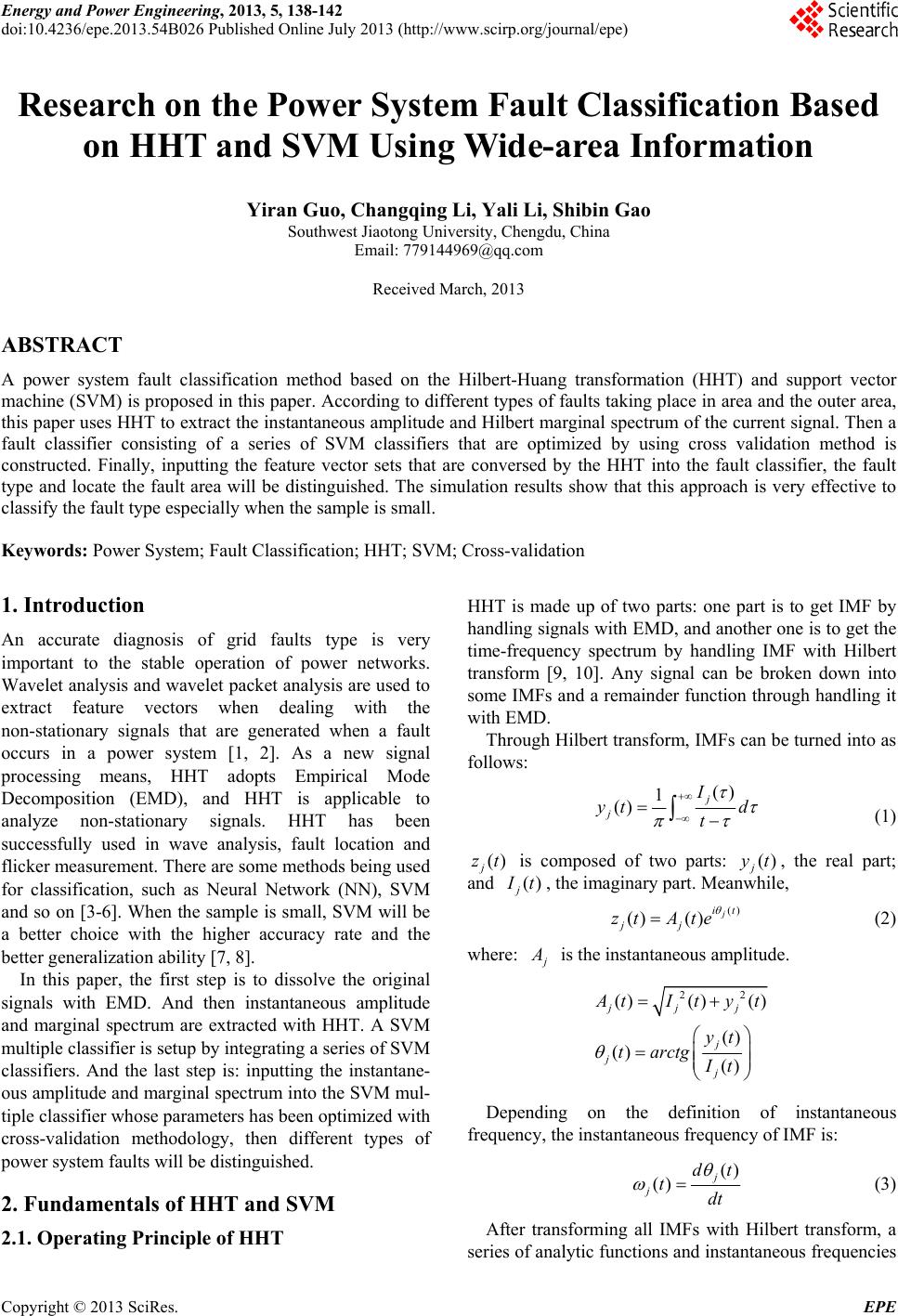Energy and Power Engineering, 2013, 5, 138-142
doi:10.4236/epe.2013.54B026 Published Online July 2013 (http://www.scirp.org/journal/epe)
Research on the Power System Fault Classification Based
on HHT and SVM Using Wide-area Information
Yiran Guo, Changqing Li, Yali Li, Shibin Gao
Southwest Jiaotong University, Chengdu, China
Received March, 2013
ABSTRACT
A power system fault classification method based on the Hilbert-Huang transformation (HHT) and support vector
machine (SVM) is proposed in this paper. According to different types of faults taking place in area and the outer area,
this paper uses HHT to extract th e instantaneous amplitude and Hilbert marginal spectrum of the current signal. Then a
fault classifier consisting of a series of SVM classifiers that are optimized by using cross validation method is
constructed. Finally, inputting the feature vector sets that are conversed by the HHT into the fault classifier, the fault
type and locate the fault area will be distinguished. The simulation results show that this approach is very effective to
classify the fault type especially when th e sample is s mall.
Keywords: Power System; Fault Classification; HHT; SVM; Cross-validation
1. Introduction
An accurate diagnosis of grid faults type is very
important to the stable operation of power networks.
Wavelet analysis and wavelet pa cket analysis are used to
extract feature vectors when dealing with the
non-stationary signals that are generated when a fault
occurs in a power system [1, 2]. As a new signal
processing means, HHT adopts Empirical Mode
Decomposition (EMD), and HHT is applicable to
analyze non-stationary signals. HHT has been
successfully used in wave analysis, fault location and
flicker measurement. There are some methods being used
for classification, such as Neural Network (NN), SVM
and so on [3-6]. When the sample is small, SVM will be
a better choice with the higher accuracy rate and the
better generalization ability [7, 8].
In this paper, the first step is to dissolve the original
signals with EMD. And then instantaneous amplitude
and marginal spectrum are extracted with HHT. A SVM
multiple classifier is setup by integrating a series of SVM
classifiers. And the last step is: inputting the instantane-
ous amplitude and marginal sp ectrum into the SVM mul-
tiple classifier whose parameters has been optimized with
cross-validation methodology, then different types of
power system faults will be distinguished.
2. Fundamentals of HHT and SVM
2.1. Operating Principle of HHT
HHT is made up of two parts: one part is to get IMF by
handling signals with EMD, and another one is to get the
time-frequency spectrum by handling IMF with Hilbert
transform [9, 10]. Any signal can be broken down into
some IMFs and a remainder function through hand ling it
with EMD.
Through Hilbert transform, IMFs can be turned in to as
follows:
()
1
() j
j
I
y
t
t

d





 (1)
()
j
zt is composed of two parts: , the real part;
and ()
j
yt
()
j
I
t, the imaginary part. Meanwhile,
()
()() j
it
jj
zt Ate

 (2)
where:
j
A
is the instantaneous amplitud e .
22
()() ()
()
() ()
jjj
j
jj
A
tIty
yt
tarctg
It






t
Depending on the definition of instantaneous
frequency, the i nstant a ne o us f req ue ncy of I M F is:
()
() j
j
dt
tdt

  (3)
After transforming all IMFs with Hilbert transform, a
series of analytic functions and instantaneous frequencies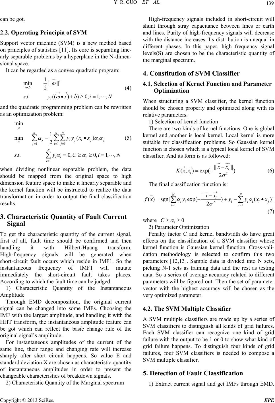

Y. R. GUO ET AL. 139
can be got.
2.2. Operating Principia of SVM
Support vector machine (SVM) is a new method based
on principles of statistics [11]. Its core is separating line-
arly separable problems by a hyperplane in the N-dimen-
sional space.
It can be regarded as a convex quadratic program:
2
,
1
min|| ||
2
..(())0,1, ,
b
i
s
tyxbi


  N


  (4)
and the qu adratic programmin g problem can be rewritten
as an optimization problem:
111
1
min
1
min( )
2
. .0,0,1,,
NNN
jijijij
jij
N
ii i
i
yy xx
s
tyCi







 

N
 (5)
when dividing nonlinear separable problem, the data
should be mapped from the original space to high
dimension feature space to make it linearly separable and
the kernel function will be instructed to realize the data
transformation in order to output the final classification
results.
3. Characteristic Quantity of Fault Current
Signal
To get the characteristic quantity of the current signal,
first of all, fault time should be confirmed and then
handling it with Hilbert-Huang transform.
High-frequency signals will be generated when
short-circuit fault occurs which reside in IMF1. So the
instantaneous frequency of IMF1 will mutate
immediately the short-circuit fault takes places.
According to which the fault time can be judged.
1) Characteristic Quantity of the Instantaneous
Amplitude
Through EMD decomposition, the original current
signal can be changed into some IMFs. Choosing the
IMF with the largest amplitude, and handling it with the
HHT transform, the instantaneous amplitude feature can
be got which can reflect the basic change rule of the
original signal’s amplitude.
For instantaneous amplitudes of the current of the
same line, their range and changing rate will increase
sharply after short circuit happens. So value E and
standard deviation X are chosen as characteristic q uantity
of instantaneous amplitudes in order to present the
changeable characteristics of breakdown signals.
2) Characteristic Quantity of the Marginal spectrum
High-frequency signals included in short-circuit will
shunt through stray capacitance between lines or earth
and lines. Purity of high-frequency signals will decrease
with the distance increases. Its distribution is unequal in
different phases. In this paper, high frequency signal
levels(S) are chosen to be the characteristic quantity of
the marginal spectrum.
4. Constitution of SVM Classifier
4.1. Selection of Kernel Function and Parameter
Optimization
When structuring a SVM classifier, the kernel function
should be chosen properly and optimized along with its
relative parameters.
1) Selection of kernel function
There are two kinds of kernel functions. One is global
kernel and another is local kernel. Local kernel is more
suitable for classification problems. So Gaussian kernel
function is chosen which is a typical local kernel of SVM
classifier. And its form is as followed:
2
|| ||
( ,)exp()
2i
i
x
x
Kxx






 (6)
The final classification function is:
2
11
|| ||
( )sgn[exp()()]
2
NN
i
iiiii ij
ii
xx
f
xy yyx 





x




(7)
where 0
i
C


2) Parameter Optimization
Penalty factor C and kernel bandwidth do have great
effects on the classification of a SVM classifier whose
kernel function is Gaussian kernel function. Cross-vali-
dation methodology is selected to confirm this two
parameters [12,13]. Sample data is divided into N sets,
picking N-1 sets as training data and the rest as testing
data. So a series of average accuracy related to different
parameters will be figured out. Then the set of parameter
vector with the highest accuracy will be chosen as the
very optimized paramet e r.
4.2. The SVM Multiple Classifier
A SVM multiple classifiers are made up by a series of
SVM classifiers to distinguish all kinds of grid failures.
Each SVM classifier can recognize one kind of grid
failure with the output to be 1 or 0 to show what kind of
grid failure happens. To distinguish four kinds of grid
failures, four SVM classifiers is needed to compose a
SVM multiple classifier.
5. Detection of Fault Classification
1) Extract current signal and get IMFs through EMD.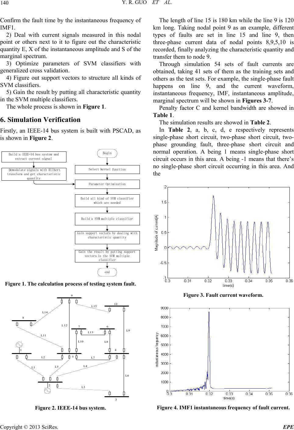

Y. R. GUO ET AL.
140
Confirm the fault time by the instantan eous frequency of
IMF1.
2) Deal with current signals measured in this nodal
point or others next to it to figure out the characteristic
quantity E, X of the instantaneous amplitud e and S of the
marginal spectrum.
3) Optimize parameters of SVM classifiers with
generalized cross validation.
4) Figure out support vectors to structure all kinds of
SVM classifiers.
5) Gain the result by putting all characteristic quantity
in the SVM multiple classifiers.
The whole process is shown in Figure 1.
6. Simulation Verification
Firstly, an IEEE-14 bus system is built with PSCAD, as
is shown in Figure 2.
Figure 1. The calculation process of testing system fault.
L1
L2
L3
L4
L5
L7
L6
L8
L9
L10
L11
L12 7
L14
L15
8
10
5
41
2
3
9
L13
6
Figure 2. IEEE-14 bus system.
The length of line 15 is 180 km while the line 9 is 120
km long. Taking nodal point 9 as an example, different
types of faults are set in line 15 and line 9, then
three-phase current data of nodal points 8,9,5,10 is
recorded, finally analyzing the characteristic qu antity and
transfer them to node 9.
Through simulation 54 sets of fault currents are
obtained, taking 41 sets of them as the training sets and
others as the test sets. For example, the single-phase fault
happens on line 9, and the current waveform,
instantaneous frequency, IMF, instantaneous amplitude,
marginal spectrum will be shown in Figures 3-7.
Penalty factor C and kernel bandwidth are showed in
Table 1.
The simulation results are showed in Table 2.
In Table 2, a, b, c, d, e respectively represents
single-phase short circuit, two-phase short circuit, two-
phase grounding fault, three-phase short circuit and
normal operation. A being 1 means single-phase short
circuit occurs in this area. A being -1 means that there’s
no single-phase short circuit occurring in this area. And
the
Figure 3. Fault current waveform.
Figure 4. IMF1 instantaneous frequency of fault current.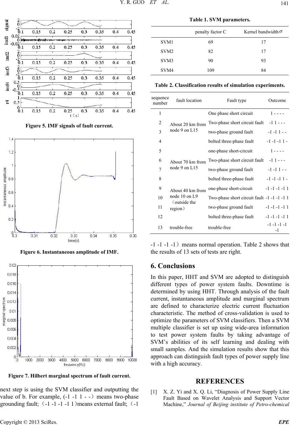

Y. R. GUO ET AL. 141
Figure 5. IMF signals of fault current.
Figure 6. Instantaneous amplitude of IMF.
Figure 7. Hilbert marginal spectrum of fault current.
next step is using the SVM classifier and outputting the
value of b. For example, (-1 -1 1 - -）means two-phase
groundi n g fault; （-1 -1 -1 -1 1）means external fault; （-1
Table 1. SVM parameters.
penalty factor C Kernel bandwidth

SVM1 69 17
SVM2 82 17
SVM3 90 93
SVM4 109 84
Table 2. Classification results of simulation experiments.
sequence
number fault location Fault type Outcome
1 One phase short circuit 1 - - - -
2 Two-phase short c ircuit fault-1 1 - - -
3 two-phase ground fault -1 -1 1 - -
4
About 20 km from
node 9 on L15
bolted three-phase fault -1 -1 -1 1 -
5 one-phase short-circuit 1 - - - -
6 Two-phase short c ircuit fault-1 1 - - -
7 two-phase ground fault -1 -1 1 - -
8
About 70 km from
node 9 on L15
bolted three-phase fault -1 -1 -1 1 -
9 one-phase short-circuit -1 -1 -1 -1 1
10 Two-phase short c ircuit fault-1 -1 -1 -1 1
11 two-phase ground fault -1 -1 -1 -1 1
12
About 40 km from
node 10 on L9
（outside the
region）
bolted three-phase fault -1 -1 -1 -1 1
13 trouble-free trouble-free -1 -1 -1 -1
-1
-1 -1 -1 -1）means normal operation. Table 2 shows that
the results of 13 sets of tests are right.
6. Conclusions
In this paper, HHT and SVM are adopted to distinguish
different types of power system faults. Downtime is
determined by using HHT. Through analysis of the fault
current, instantaneous amplitude and marginal spectrum
are defined to characterize electric current fluctuation
characteristic. The method of cross-validation is used to
optimize the parameters of SVM classifiers. Then a SVM
multiple classifier is set up using wide-area information
to test power system faults by taking advantage of
SVM’s abilities of its self learning and dealing with
small samples. And the simulation results show that this
approach can distinguish fault types of power supply line
with a high accuracy.
REFERENCES
[1] X. Z. Yi and X. Q. Li, “Diagnosis of Power Supply Line
Fault Based on Wavelet Analysis and Support Vector
Machine,” Journal of Beijing institute of Petro-chemical

Y. R. GUO ET AL.
142
Technology, Vol. 13, No. 3, 2005, pp. 36-40.
[2] Y. H. Liu, Y. Y. Wang and Z. H. Song, “Adaptive Fault
Feature Extraction Based on Stationary Wavelet Packet
Decomposition and Hilbert Transform,” Transacions of
China Electrotechnical Society, Vol. 24, No. 2, 2009, pp.
145-149.
[3] X. L. Zhang, X. J. Zeng, H. J. Ma, et al., “Power Grid
Faults Location with Traveling Wave Based on
Hilbert-Huang Transform,” Automation of electric power
systems, Vol. 32, No. 8, 2008, pp. 64-67
[4] S. Han, L. Q. He, B. Sun, et al., “Hilbert-Huang
Transform Based Nonlinear and Non-Stationary Analysis
of Power System Low Frequency Oscillation and Its
Application,” Power System Technology, Vol. 32, No. 4,
2008, pp. 56-60.
[5] Y. X. Su, Z. G. Liu, K. L. Li, et al., “Application of
Hilbert-Huang Transform in Harmonic Detection of
Electrified Railway,” Power System Technology, Vol. 32,
No. 18, 2008, pp. 30-35
[6] Z. J. Kang, L. Xu, J. C. Fan, et al., “Fault Location for
High Voltage Transmission Lines With the Series
Compensation Capacitor Based on Hilbert-Huang
Transform and Neural Network,” Power System
Technology, Vol. 33, No. 20, 2009, pp. 142-146
[7] J. Manikandan and B. Venkataramani, “Design of a
Modified One-against-all SVM Classifier,” Proceedings
of the 2009 IEEE International Conference on Systems,
man, and cybernetics, 2009, pp. 1869-1874
[8] D. C. Yang, C. Rehtanz, Y. Li, W. Tang and R. Q. Qu,
“Researching on Low Frequency Oscillation in Power
System Based on Improved HHT Algorithm,”
Proceedings of the CSEE, Vol. 31, No.10, 2011,
pp.102-108.
[9] H. Jiang, X. Q. Wang and J. C. Peng, “Method to
Measure Voltage Flicker Based on Hilbert-Huang
Transform,” Power System Technology, Vol. 35, No. 9,
2012, pp. 250-256.
[10] Q. Zhang and Y. Q. Yang, “Research of the Kernel
Fuction of Support Vector Machine,” Electric Power
Science and Engineering, Vol. 28, No. 5, 2012, pp. 42-45.
[11] T. Y. Li, C. L. Chen, W. L. Cheng, et al., “Application of
cross Validation in Power Quality Denoisin,” Automation
of Electric Power Systems, Vol. 319, No. 16, 2007, pp.
75-78.
[12] J. Ma, X.Wang and Z. P. Wang, “A New Fault Phase
Identification Method Based on Phase Current
Difference,” Proceedings of the CSEE, Vol. 31, No. 10,
2011, pp. 102-108
[13] Y. Wang, Y. X. Zhang and S. X. Xu, “Fault Location and
Phase Selection for Parallel Transmission Lines Based on
Wide Area Measurement System,” Automation of Electric
Power Systems, Vol. 34, No. 6, 2010, pp. 65-69.