J. Biomedical Science and Engineering, 2011, 4, 62-69
doi:10.4236/jbise.2011.41008 Published Online January 2011 (http://www.SciRP.org/journal/jbise/
JBiSE
).
Published Online January 2011 in SciRes. http://www.scirp.org/journal/JBiSE
Comparison of SVM and ANN for classification of eye events
in EEG
Rajesh Singla1, Brijil Chambayil1, Arun Khosla2, Jayashr e e Santosh3
1Department of Instrumentation and Control Engineering National Institute of Technology, Jalandhar, India;
2Department of Electronics and Communication Engineering National Institute of Technology, Jalandhar, India;
3Computer Services Centre, IIT, New Delhi, India.
Received 11 November 2010; revised 17 November 2010; accepted 19 November 2010.
ABSTRACT
The eye events (eye blink, eyes close and eyes open)
are usually considered as biological artifacts in the
electroencephalographic (EEG) signal. One can con-
trol his or her eye blink by proper training and hence
can be used as a control signal in Brain Computer
Interface (BCI) applications. Support vector ma-
chines (SVM) in recent years proved to be the best
classification tool. A comparison of SVM with the
Artificial Neural Network (ANN) always provides
fruitful results. A one-against-all SVM and a multi-
layer ANN is trained to detect the eye events. A com-
parison of both is made in this paper.
Keywords: ANN; BCI; EEG; Eye Event; Kurtosis; SVM
1. INTRODUCTION
The electroencephalogram, or EEG, consists of the elec-
trical activity of relatively large neuronal populations
that can be recorded from the scalp. In healthy adults,
the amplitudes and frequencies of such signals change
from one state of a human to another, such as wakeful-
ness and sleep. The characteristics of the waves also
change with age. There are five major brain waves dis-
tinguished by their different frequency ranges. These
frequency bands from low to high frequencies respec-
tively are called delta (δ), theta (θ), alpha (α), beta (β),
and gamma (γ).
The main artifacts in EEG can be divided into pa-
tient-related (physiological) and system artifacts. The
patient-related or internal artifacts are body move-
ment-related, EMG, ECG (and pulsation), EOG, ballis-
tocardiogram and sweating. The system artifacts are
50/60 Hz power supply interference, impedance fluctua-
tions, cable defects, electrical noise from the electronic
components and unbalanced impedances of the elec-
trodes.
Eye events (eye blink, eyes close and eyes open) are
normally considered as physiological artifacts in the
EEG. But if we consider in a BCI point of view, these
signals, although artifacts, can be used as good control
signals. Eye blink signals can be used in BCI applica-
tions like virtual keyboard while the eye close and eyes
open signals can be used for folding and opening electric
foldable hospital beds.
SVMs (Support Vector Machines) are a useful tech-
nique for data classification. The foundations of Support
Vector Machines have been developed by Vapnik (1995)
and are gaining popularity due to many attractive fea-
tures, and promising empirical performance. The SVM
belongs to a class of machine learning algorithms that
are based on linear classifiers and the “kernel trick”. The
aim of Support Vector classification is to devise a com-
putationally efficient way of learning ‘good’ separating
hyperplanes in a high dimensional feature space, where
‘good’ hyperplanes are ones optimizing the generaliza-
tion bounds, and ‘computationally efficient’ mean algo-
rithms able to deal with sample sizes of the order of
100000 instances [8].
2. EYE EVENT CHARACTERISTICS
The eye event signals includes: eye blink, eyes close and
eyes open. Eye blinks are typically characterized by
peaks with relatively strong voltages. There is also cer-
tain variability in the amplitude of the peaks of a specific
individual, more variability between different subjects.
Eye blinks can be classified as short blinks if the dura-
tion of blink is less than 200 ms or long blinks if it is
greater or equal to 200 ms.
Eye blinks can be classified into three types: reflexive,
voluntary and spontaneous. The eye blink reflexive is
the simplest response and does not require the involve-
ment of cortical structures. In contrast, voluntary eye
blinking (i.e. purposely blinking due to predetermined
condition) involves multiple areas of the cerebral cortex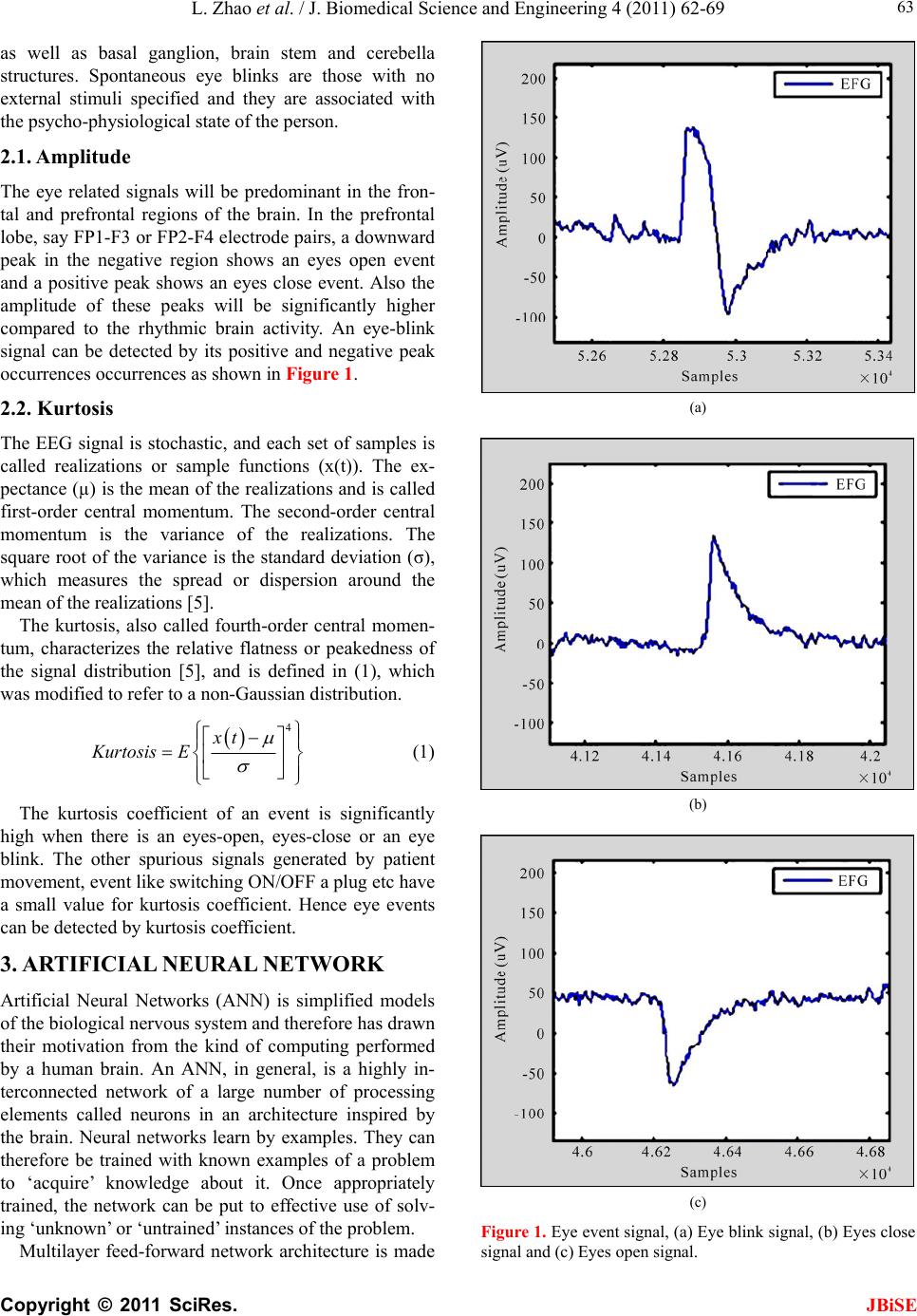

L. Zhao et al. / J. Biomedical Science and Engineering 4 (2011) 62-69
63
as well as basal ganglion, brain stem and cerebella
structures. Spontaneous eye blinks are those with no
external stimuli specified and they are associated with
the psycho-physiological state of the person.
2.1. Amplitude
The eye related signals will be predominant in the fron-
tal and prefrontal regions of the brain. In the prefrontal
lobe, say FP1-F3 or FP2-F4 electrode pairs, a downward
peak in the negative region shows an eyes open event
and a positive peak shows an eyes close event. Also the
amplitude of these peaks will be significantly higher
compared to the rhythmic brain activity. An eye-blink
signal can be detected by its positive and negative peak
occurrences occurrences as shown in Figure 1.
2.2. Kurtosis
The EEG signal is stochastic, and each set of samples is
called realizations or sample functions (x(t)). The ex-
pectance (µ) is the mean of the realizations and is called
first-order central momentum. The second-order central
momentum is the variance of the realizations. The
square root of the variance is the standard deviation (σ),
which measures the spread or dispersion around the
mean of the realizations [5].
The kurtosis, also called fourth-order central momen-
tum, characterizes the relative flatness or peakedness of
the signal distribution [5], and is defined in (1), which
was modified to refer to a non-Gaussian distribution.

4
xt
Kurtosis E







 




(1)
The kurtosis coefficient of an event is significantly
high when there is an eyes-open, eyes-close or an eye
blink. The other spurious signals generated by patient
movement, event like switching ON/OFF a plug etc have
a small value for kurtosis coefficient. Hence eye events
can be detected by kurtosis coefficient.
3. AR TIFICIAL NEURAL NETWORK
Artificial Neural Networks (ANN) is simplified models
of the biological nervous system and therefore has drawn
their motivation from the kind of computing performed
by a human brain. An ANN, in general, is a highly in-
terconnected network of a large number of processing
elements called neurons in an architecture inspired by
the brain. Neural networks learn by examples. They can
therefore be trained with known examples of a problem
to ‘acquire’ knowledge about it. Once appropriately
trained, the network can be put to effective use of solv-
ing ‘unknown’ or ‘untrained’ instances of the problem.
Multilayer feed-forward network architecture is made
(a)
(b)
(c)
Figure 1. Eye event signal, (a) Eye blink signal, (b) Eyes close
signal and (c) Eyes open signal.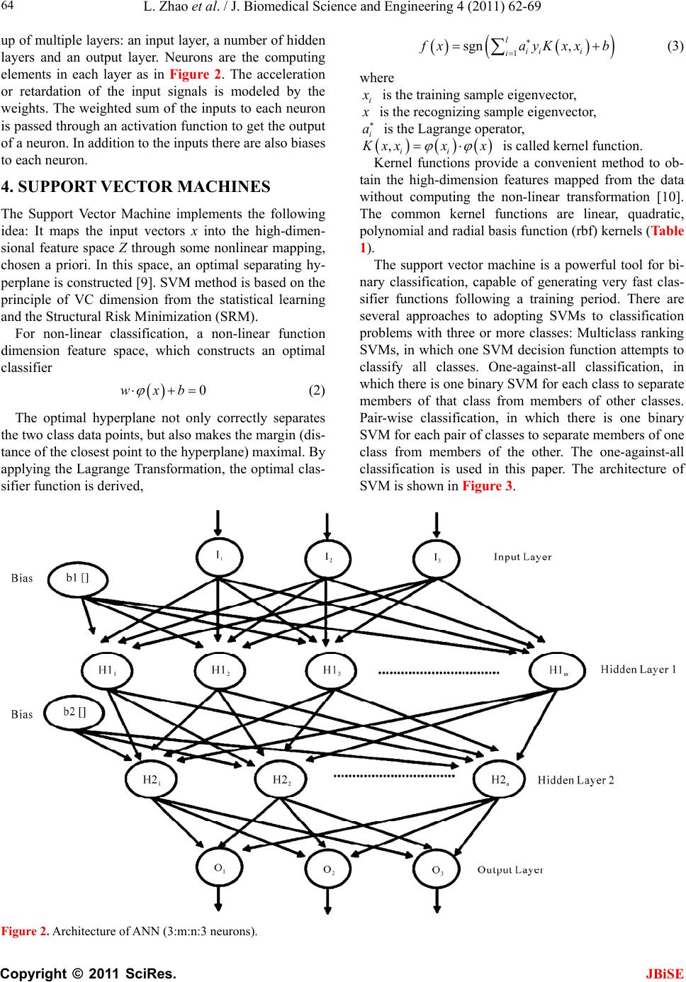

L. Zhao et al. / J. Biomedical Science and Engineering 4 (2011) 62-69
64
t layer, a number of hidden
VECTOR MACHINES
llowing
r function
di
(2)
The optimal hyperplane not only correctly separates
th
 


1
sgn ,
l
ii i
i
f
xayKxx


up of multiple layers: an inpub


 (3)
layers and an output layer. Neurons are the computing
elements in each layer as in Figure 2. The acceleration
or retardation of the input signals is modeled by the
weights. The weighted sum of the inputs to each neuron
is passed through an activation function to get the output
of a neuron. In addition to the inputs there are also biases
to each neuron.
4. SUPPORT
where
i
x
is the training sample eigenvector,
x
is the recognizing sample eigenvector,
i
a

is the Lagrange operator,






,ii
K
xxx x   is called kernel function.
Kernel functions provide a convenient method to ob-
tain the high-dimension features mapped from the data
without computing the non-linear transformation [10].
The common kernel functions are linear, quadratic,
polynomial and radial basis function (rbf) kernels (Table
1).
The Support Vector Machine implements the fo
idea: It maps the input vectors x into the high-dimen-
sional feature space Z through some nonlinear mapping,
chosen a priori. In this space, an optimal separating hy-
perplane is constructed [9]. SVM method is based on the
principle of VC dimension from the statistical learning
and the Structural Risk Minimization (SRM).
For non-linear classification, a non-linea
The support vector machine is a powerful tool for bi-
nary classification, capable of generating very fast clas-
sifier functions following a training period. There are
several approaches to adopting SVMs to classification
problems with three or more classes: Multiclass ranking
SVMs, in which one SVM decision function attempts to
classify all classes. One-against-all classification, in
which there is one binary SVM for each class to separate
members of that class from members of other classes.
Pair-wise classification, in which there is one binary
SVM for each pair of classes to separate members of one
class from members of the other. The one-against-all
classification is used in this paper. The architecture of
SVM is shown in Figure 3.
mension feature space, which constructs an optimal
classifier

0wxb  
e two class data points, but also makes the margin (dis-
tance of the closest point to the hyperplane) maximal. By
applying the Lagrange Transformation, the optimal clas-
sifier function is derived,
Figure 2. Architecture of ANN (3:m:n:3 neurons).
JBiSE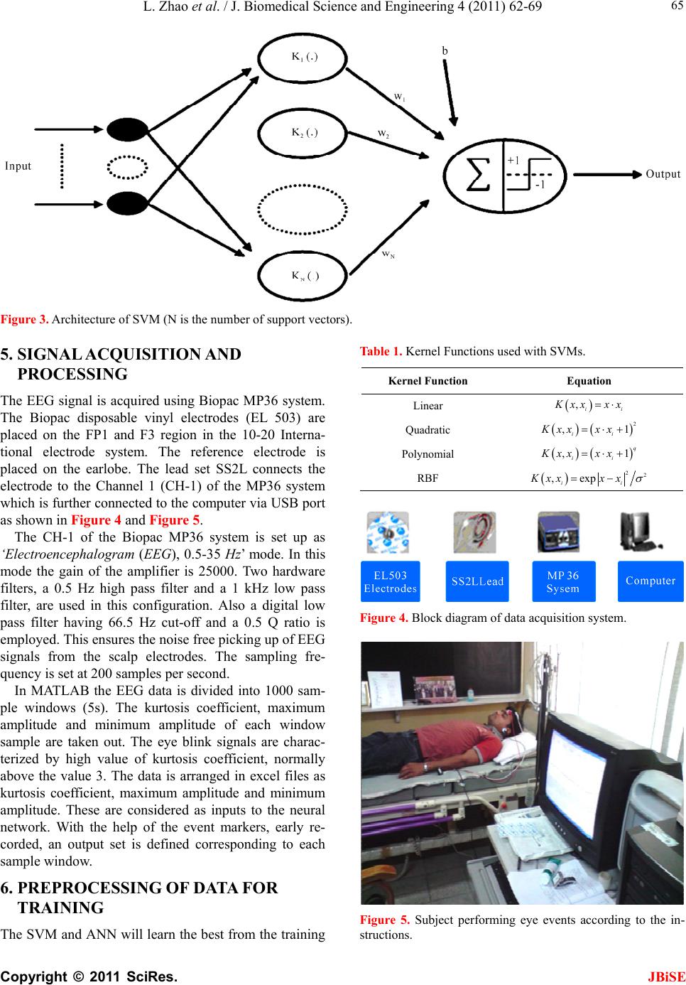

L. Zhao et al. / J. Biomedical Science and Engineering 4 (2011) 62-69
65
Figure 3. Architecture of SVM (N is the number of support vectors).
The red using Biopac MP36 system.
system is set up as
‘E
into 1000 sam-
pl
NG OF DATA FOR
Th will learn the best from the training
Table 1. Kernel Functions used with SVMs.
tion
5. SIGNAL ACQUISITION AND
PROCESSING
EEG signal is acqui
The Biopac disposable vinyl electrodes (EL 503) are
placed on the FP1 and F3 region in the 10-20 Interna-
tional electrode system. The reference electrode is
placed on the earlobe. The lead set SS2L connects the
electrode to the Channel 1 (CH-1) of the MP36 system
which is further connected to the computer via USB port
as shown in Figure 4 and Figure 5.
The CH-1 of the Biopac MP36
lectroencephalogram (EEG), 0.5-35 Hz’ mode. In this
mode the gain of the amplifier is 25000. Two hardware
filters, a 0.5 Hz high pass filter and a 1 kHz low pass
filter, are used in this configuration. Also a digital low
pass filter having 66.5 Hz cut-off and a 0.5 Q ratio is
employed. This ensures the noise free picking up of EEG
signals from the scalp electrodes. The sampling fre-
quency is set at 200 samples per second.
In MATLAB the EEG data is divided
e windows (5s). The kurtosis coefficient, maximum
amplitude and minimum amplitude of each window
sample are taken out. The eye blink signals are charac-
terized by high value of kurtosis coefficient, normally
above the value 3. The data is arranged in excel files as
kurtosis coefficient, maximum amplitude and minimum
amplitude. These are considered as inputs to the neural
network. With the help of the event markers, early re-
corded, an output set is defined corresponding to each
sample window.
6. PREPROCESSI
TRAINING
e SVM and ANN
Kernel Function Equa
Linear

,ii
K
xx xx
Quadratic
Polyno
 
2
,1
ii
Kxx xx
mial
 
,1
q
ii
Kxx xx
RBF

22
,exp
ii
Kxxx x


Figure 4. Block diagram of data acquisition system.
Figure 5. Subject performing eye events according to the in-
structions.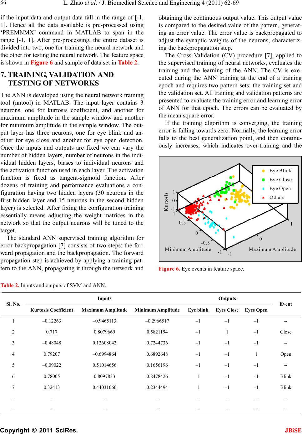

L. Zhao et al. / J. Biomedical Science and Engineering 4 (2011) 62-69
66
Thnetwork training
if the input data and output data fall in the range of [-1,
1]. Hence all the data available is pre-processed using
‘PREMNMX’ command in MATLAB to span in the
range [-1, 1]. After pre-processing, the entire dataset is
divided into two, one for training the neural network and
the other for testing the neural network. The feature space
is shown in Figure 6 and sample of data set in Table 2.
7. TRAINING, VA LIDATION AND
TESTING OF NETWORKS
e ANN is developed using the neural
tool (nntool) in MATLAB. The input layer contains 3
neurons, one for kurtosis coefficient, and another for
maximum amplitude in the sample window and another
for minimum amplitude in the sample window. The out-
put layer has three neurons, one for eye blink and an-
other for eye close and another for eye open detection.
Once the inputs and outputs are fixed we can vary the
number of hidden layers, number of neurons in the indi-
vidual hidden layers, biases to individual neurons and
the activation function used in each layer. The activation
function is fixed as tangent-sigmoid function. After
dozens of training and performance evaluations a con-
figuration having two hidden layers (30 neurons in the
first hidden layer and 15 neurons in the second hidden
layer) is selected. After fixing the configuration training
essentially means adjusting the weight matrices in the
network so that the output neurons will be tuned to the
target.
The standard ANN supervised training algorithm for
error backpropagation [7] consists of two steps: the for-
ward propagation and the backpropagation. The forward
propagation step is achieved by applying a training pat-
tern to the ANN, propagating it through the network and
obtaining the continuous output value. This output value
is compared to the desired value of the pattern, generat-
ing an error value. The error value is backpropagated to
adjust the synaptic weights of the neurons, characteriz-
ing the backpropagation step.
The Cross Validation (CV) procedure [7], applied to
the supervised training of neural networks, evaluates the
training and the learning of the ANN. The CV is exe-
cuted during the ANN training at the end of a training
epoch and requires two pattern sets: the training set and
the validation set. All training and validation patterns are
presented to evaluate the training error and learning error
of ANN for that epoch. The errors can be evaluated by
the mean square error.
If the training algorithm is converging, the training
error is falling towards zero. Normally, the learning error
falls to the best generalization point, and then continu-
ously increases, which indicates over-training and the
Figure 6. Eye events in feature space.
able 2. Inputs and outputs of SVM and ANN. T
Inputs Outputs
Sl. No. Kurtosis Coefficient MaximudeMinimum AmplitudeEye blinkEEyes Open Event
um Amplityes Close
1 –0.12263 –0.9465113 –0.2966517 –1 –1 –1 --
2 0.717 0.8079669 0.5821194 –1 1 –1 Close
–
Open
Blink
-- -- -- -- -- -- -- --
3 0.480480.12608042 0.7244736 –1 –1 –1 --
4 0.79207 –0.6994864 0.6892648 –1 –1 1
5 –0.09022 0.51014656 0.1656196 –1 –1 –1 --
6 0.78005 0.8097833 0.8478426 1 –1 –1
7 0.32413 0.44031066 0.2344494 1 –1 –1 Blink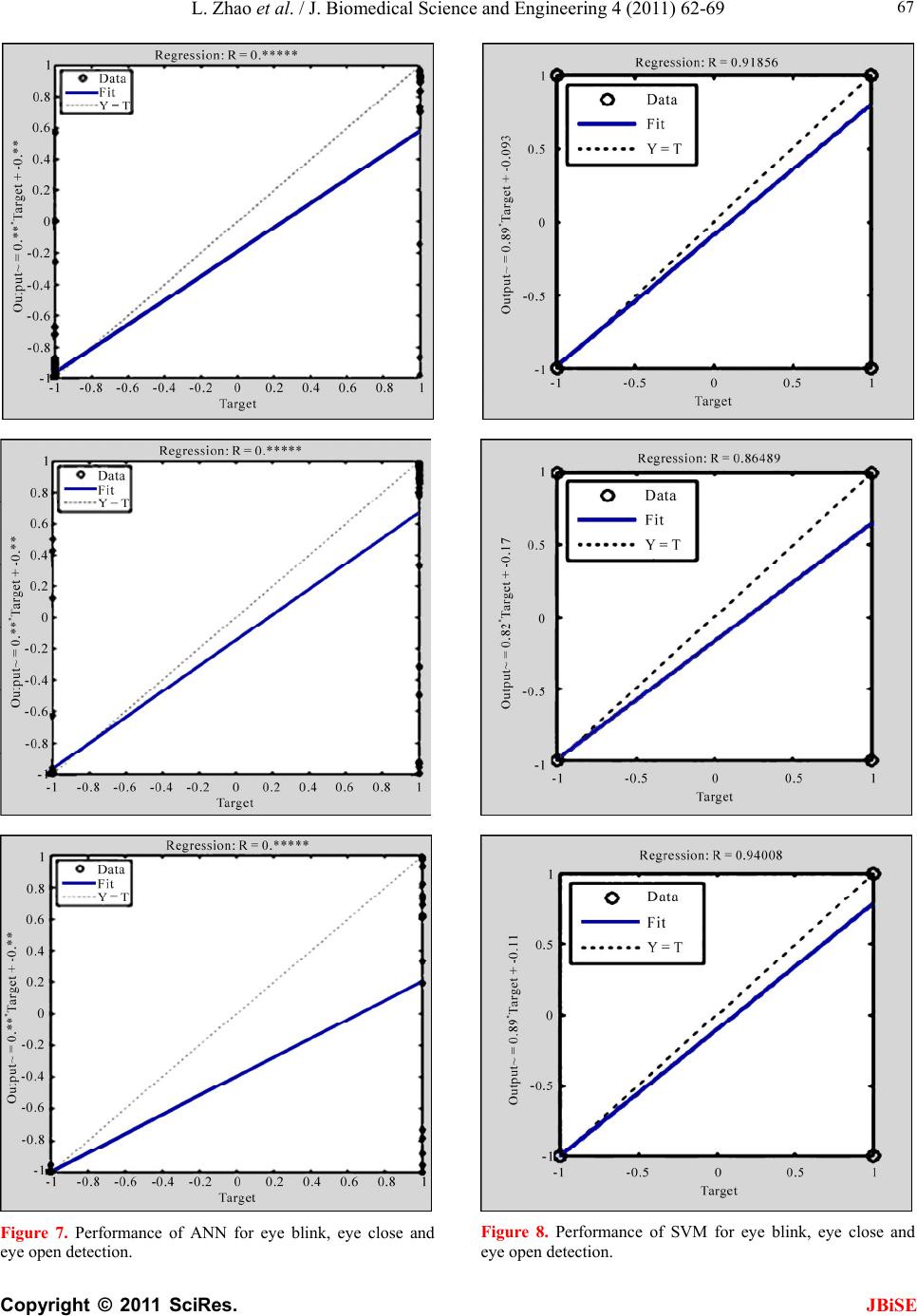
-- -- -- -- -- -- -- --

L. Zhao et al. / J. Biomedical Science and Engineering 4 (2011) 62-69
67
Figure 8. Performance of SVM for eye blink, eye close and
eye open detection.
Figure 7. Performance of ANN for eye blink, eye close and
eye open detection.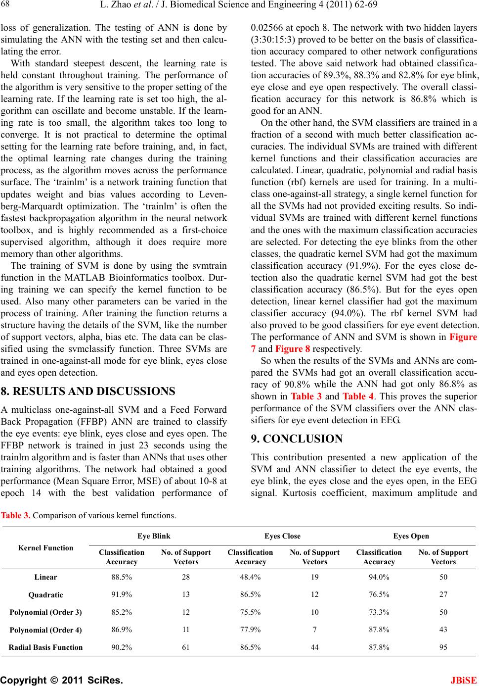

L. Zhao et al. / J. Biomedical Science and Engineering 4 (2011) 62-69
68
loss of generalization. The testing of ANN is done by
simulating the ANN with the testing set and then calcu-
lating the error.
With standard steepest descent, the learning rate is
held constant throughout training. The performance of
the algorithm is very sensitive to the proper setting of the
learning rate. If the learning rate is set too high, the al-
gorithm can oscillate and become unstable. If the learn-
ing rate is too small, the algorithm takes too long to
converge. It is not practical to determine the optimal
setting for the learning rate before training, and, in fact,
the optimal learning rate changes during the training
process, as the algorithm moves across the performance
surface. The ‘trainlm’ is a network training function that
updates weight and bias values according to Leven-
berg-Marquardt optimization. The ‘trainlm’ is often the
astest backpropagation algorithm in the neural networ
oolbox, and is highly recommended as a first-choice
supervised algorithm, although it does require more
memory than other algorithms.
The training of SVM is done by using the svmtrain
function in the MATLAB Bioinformatics toolbox. Dur-
ing training we can specify the kernel function to be
used. Also many other parameters can be varied in the
process of training. After training the function returns a
structure having the details of the SVM, like the number
of support vectors, alpha, bias etc. The data can be clas-
sified using the svmclassify function. Three SVMs are
trained in one-against-all mode for eye blink, eyes close
and eyes open detection.
8. RESULT S AND DISCUSSIONS
A multiclass one-against-all SVM and a Feed Forward
Back Propagation (FFBP) ANN are trained to classif
rained in just 23 seconds using the
ean Square Error, MSE) of about 10-8 at
ep
r network configurations
te
tic, polynomial and radial basis
In a multi-
function for
ile the ANN had got only 86.8% as
sh
f
t
k
y
the eye events: eye blink, eyes close and eyes open. The
FFBP network is t
trainlm algorithm and is faster than ANNs that uses other
training algorithms. The network had obtained a good
performance (M
och 14 with the best validation performance of
0.02566 at epoch 8. The network with two hidden layers
(3:30:15:3) proved to be better on the basis of classifica-
tion accuracy compared to othe
Table 3. Comparison of various kernel functions.
Eye Blink
sted. The above said network had obtained classifica-
tion accuracies of 89.3%, 88.3% and 82.8% for eye blink,
eye close and eye open respectively. The overall classi-
fication accuracy for this network is 86.8% which is
good for an ANN.
On the other hand, the SVM classifiers are trained in a
fraction of a second with much better classification ac-
curacies. The individual SVMs are trained with different
kernel functions and their classification accuracies are
calculated. Linear, quadra
function (rbf) kernels are used for training.
class one-against-all strategy, a single kernel
all the SVMs had not provided exciting results. So indi-
vidual SVMs are trained with different kernel functions
and the ones with the maximum classification accuracies
are selected. For detecting the eye blinks from the other
classes, the quadratic kernel SVM had got the maximum
classification accuracy (91.9%). For the eyes close de-
tection also the quadratic kernel SVM had got the best
classification accuracy (86.5%). But for the eyes open
detection, linear kernel classifier had got the maximum
classifier accuracy (94.0%). The rbf kernel SVM had
also proved to be good classifiers for eye event detection.
The performance of ANN and SVM is shown in Figure
7 and Figure 8 respectively.
So when the results of the SVMs and ANNs are com-
pared the SVMs had got an overall classification accu-
racy of 90.8% wh
own in Ta ble 3 and Table 4. This proves the superior
performance of the SVM classifiers over the ANN clas-
sifiers for eye event detection in EEG.
9. CONCLUSION
This contribution presented a new application of the
SVM and ANN classifier to detect the eye events, the
eye blink, the eyes close and the eyes open, in the EEG
signal. Kurtosis coefficient, maximum amplitude and
Eyes Close Eyes Open
Kernel Function Classification
Accuracy No. of Support Vectors Classi Accu
fication
racy No. of Support Vectors Classification Accuracy No. of Support Vectors
Linear 88.5% 28 48.4% 19 94.0% 50
Quadratic 91.9% 13
Polynomial (O r de r 3) 85.2% 12
Polynomial (O r de r 4) 86.9% 11
Radial Basis Function 90.2% 61
86
75
77
86
.5% 12 76.5% 27
.5% 10 73.3% 50
.9% 7 87.8% 43
.5% 44 87.8% 95

L. Zhao et al. / J. Biomedical Science and Engineering 4 (2011) 62-69
69
Table 4. Comparison of SVM and ANN.
ANN Configuration
Maximum Classification
Accuracy Obtained for SVM 3:30:15:3
(neurons) 3:20:10:3 (neurons)
Eye Blink 91.9% 89.3% 71.8%
Eyes Close 86.5% 88.4% 66.1%
Eyes Open 94.0% 82.8% 84.7%
90.8% 86.8% 74.2% Overall
minimumlitude in a saare success-
fully usain the netwo detect the event
signalsM provideaximum cification
accuracy of 90.
T SVMifier have better per-
foN cl. The classis devel-
opedeveloCI systemhat uses
ygnaked-in
myotrophic lateral
sclerosis (ALS).
R
[1] Sanei, S. and Chambe(20G sig
essiley & S., Chichester.
[2] Ra., Vijayai Pa(200ral
170-172. doi:10.4236/jbise.2008.13028
amp
ed to tr
mple window
orks te ey
. The SVd a mlass
8%, while the
his proves that the
ANN provided only 86.8%.
class
rmance than the ANassifierfier
d can be used for
e events as control si
ping a B
ls, especially for loc
t
e
patients like those suffering from A
EFERENCES
rs, J.A.
ons Ltd
07) EEnal proc-
ing. John W
jasekaran, Slakshmi, G.A. 8) Neu
networks, fuzzy logic and genetic algorithms: synthesis
and applications. Prentice-Hall of India Private Limted,
New Delhi.
[3] Singla, R. and Gupta, B. (2008) Brain initiated interac-
tion. Journal of Biomedical Science and Engineering, 1,
[4] Manoilov, P. (2006) EEG eye-blinking artifacts power
spectrum analysis. Proceedings of International Confer-
ence on Computer Systems and Technologies, Bulgaria,
15-16 June 2006, IIIA. 3-1-IIIA.3-5.
[5] ki, M.A., Argoud, F.I.Mevedo, F.M.
(2008) Identifying eye blinks in EEG signal analysis.
roc5th C-
formatioology ation in cine,
30-31 May8, Shenzhen, China, 406-409.
[6] Manolakis, D.G., Ingle, V.K. and Kogon, S.M. (2005)
Statistical adaptive siocessing: Spal esti-
mation, signd array
processing. Artech House Prs, London.
Haykin, S. (1998) Neural networks: A comprehensive
foundation.tice Hall, New Jrsey.
Cristianiniand Shawe-T. (2000) An iduction
Sovierzos . and de Az
Peedings of the
n Techn International nd Applicaonference on In Biomedi
200
andgnal prectr
al modeling, adaptive filtering an
ublishe
[7]
Prene
[8] , N. aylor, Jntro
to support vector machines and other kernel-based learning
methods. Cambridge University Press, Cambridge.
[9] Vapnik, V. (1998) Statistical Learning Theory. John
Wiley & Sons, Chichester.
[10] Xie, S.-Y., Wang, P.-W., Zhang, H.-J. and Zhao, H.-T.
(2008) Research on the classification of brain function
based on SVM. The 2nd International Conference on
Bioinformatics and Biomedical Engineering, 16-18 May
2008, 1931-1934.