Multi-timescale Collaborative Optimization of Distribution, Distributed Generation and Load in Microgrid

doi:10.4236/ojapps.2013.32B003

Paper Menu >>

Journal Menu >>

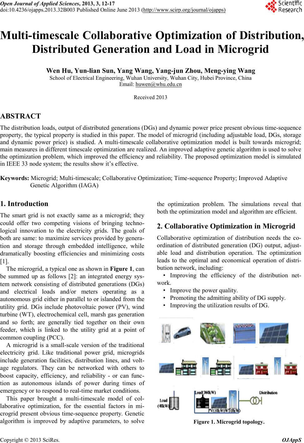
Open Journal of Applied Sciences, 2013, 3, 12-17

doi:10.4236/ojapps.2013.32B003 Published Online June 2013 (http://www.scirp.org/journal/ojapps)

Multi-timescale Collaborative Optimization of Distribution,

Distributed Generation and Load in Microgrid

Wen Hu, Yun-lian Sun, Yang Wang, Yang-jun Zhou, Meng-ying Wang

School of Electrical Engineering, Wuhan University, Wuhan City, Hubei Province, China

Email: huwen@whu.edu.cn

Received 2013

ABSTRACT

The distribution loads, output of distributed generations (DGs) and dynamic power price present obvious time-sequence

property, the typical property is studied in this paper. The model of microgrid (including adjustable load, DGs, storage

and dynamic power price) is studied. A multi-timescale collaborative optimization model is built towards microgrid;

main measures in different timescale optimization are realized. An improved adaptive genetic algorithm is used to solve

the optimization problem, which improved the efficiency and reliability. The proposed optimization model is simulated

in IEEE 33 node system; the results show it’s effective.

Keywords: Microgrid; Multi-timescale; Collaborative Optimization; Time-sequence Property; Improved Adaptive

Genetic Algorithm (IAGA)

1. Introduction

The smart grid is not exactly same as a microgrid; they

could offer two competing visions of bringing techno-

logical innovation to the electricity grids. The goals of

both are same: to maximize services provided by genera-

tion and storage through embedded intelligence, while

dramatically boosting efficiencies and minimizing costs

[1].

The microgrid, a typical one as shown in Figure 1, can

be summed up as follows [2]: an integrated energy sys-

tem network consisting of distributed generations (DGs)

and electrical loads and/or meters operating as a

autonomous grid either in parallel to or islanded from the

utility grid. DGs include photovoltaic power (PV), wind

turbine (WT), electrochemical cell, marsh gas generation

and so forth; are generally tied together on their own

feeder, which is linked to the utility grid at a point of

common coupling (PCC).

A microgrid is a small-scale version of the traditional

electricity grid. Like traditional power grid, microgrids

include generation facilities, distribution lines, and volt-

age regulators. They can be networked with others to

boost capacity, efficiency, and reliability - or can func-

tion as autonomous islands of power during times of

emergency or to respond to real-time market conditions.

This paper brought a multi-timescale model of col-

laborative optimization, for the essential factors in mi-

crogrid present obvious time-sequence property. Genetic

algorithm is improved by adaptive parameters, to solve

the optimization problem. The simulations reveal that

both the optimization model and algorithm are efficient.

2. Collaborative Optimization in Microgrid

Collaborative optimization of distribution needs the co-

ordination of distributed generation (DG) output, adjust-

able load and distribution operation. The optimization

leads to the optimal and economical operation of distri-

bution network, including:

• Improving the efficiency of the distribution net-

work.

• Improve the power quality.

• Promoting the admitting ability of DG supply.

• Improving the utilization results of DG.

Figure 1. Microgrid topology.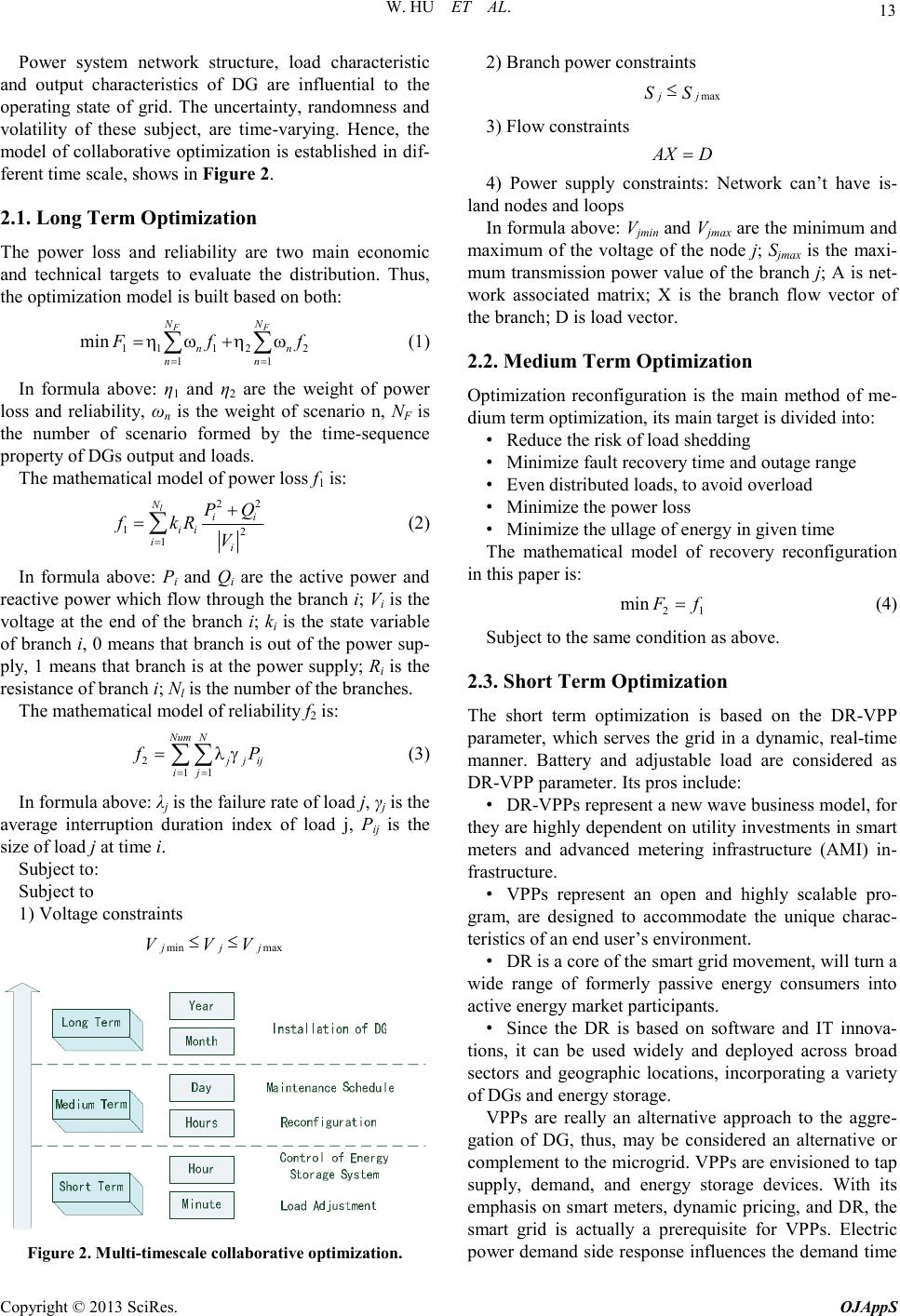

W. HU ET AL.

Power system network structure, load characteristic

and output characteristics of DG are influential to the

operating state of grid. The uncertainty, randomness and

volatility of these subject, are time-varying. Hence, the

model of collaborative optimization is established in dif-

ferent time scale, shows in Figure 2.

2.1. Long Term Optimization

The power loss and reliability are two main economic

and technical targets to evaluate the distribution. Thus,

the optimization model is built based on both:

11122

min FF

Fff

ηωηω

∑∑

(1)

In formula above: η1 and η2 are the weight of power

loss and reliability, ωn is the weight of scenario n, NF is

the number of scenario formed by the time-sequence

property of DGs output and loads.

The mathematical model of power loss f1 is:

fkR V

=∑ (2)

In formula above: Pi and Qi are the active power and

reactive power which flow through the branch i; Vi is the

voltage at the end of the branch i; ki is the state variable

of branch i, 0 means that branch is out of the power sup-

ply, 1 means that branch is at the power supply; Ri is the

resistance of branch i; Nl is the number of the branches.

The mathematical model of reliability f2 is:

211

NumN

jjij

λγ

∑∑ (3)

In formula above: λj is the failure rate of load j, γj is the

average interruption duration index of load j, Pij is the

size of load j at time i.

Subject to:

Subject to

1) Voltage constraints

minmax

jjj

VVV

≤≤

Figure 2. Multi-timescale collaborative optimization.

2) Branch power constraints

max

≤

3) Flow constraints

AXD

4) Power supply constraints: Network can’t have is-

land nodes and loops

In formula above: Vjmin and Vjmax are the minimum and

maximum of the voltage of the node j; Sjmax is the maxi-

mum transmission power value of the branch j; A is net-

work associated matrix; X is the branch flow vector of

the branch; D is load vector.

2.2. Medium Term Optimization

Optimization reconfiguration is the main method of me-

dium term optimization, its main target is divided into:

• Reduce the risk of load shedding

• Minimize fault recovery time and outage range

• Even distributed loads, to avoid overload

• Minimize the power loss

• Minimize the ullage of energy in given time

The mathematical model of recovery reconfiguration

in this paper is:

min

(4)

Subject to the same condition as above.

2.3. Short Term Optimization

The short term optimization is based on the DR-VPP

parameter, which serves the grid in a dynamic, real-time

manner. Battery and adjustable load are considered as

DR-VPP parameter. Its pros include:

• DR-VPPs represent a new wave business model, for

they are highly dependent on utility investments in smart

meters and advanced metering infrastructure (AMI) in-

frastructure.

• VPPs represent an open and highly scalable pro-

gram, are designed to accommodate the unique charac-

teristics of an end user’s environment.

• DR is a core of the smart grid movement, will turn a

wide range of formerly passive energy consumers into

active energy market participants.

• Since the DR is based on software and IT innova-

tions, it can be used widely and deployed across broad

sectors and geographic locations, incorporating a variety

of DGs and energy storage.

VPPs are really an alternative approach to the aggre-

gation of DG, thus, may be considered an alternative or

complement to the microgrid. VPPs are envisioned to tap

supply, demand, and energy storage devices. With its

emphasis on smart meters, dynamic pricing, and DR, the

smart grid is actually a prerequisite for VPPs. Electric

power demand side response influences the demand time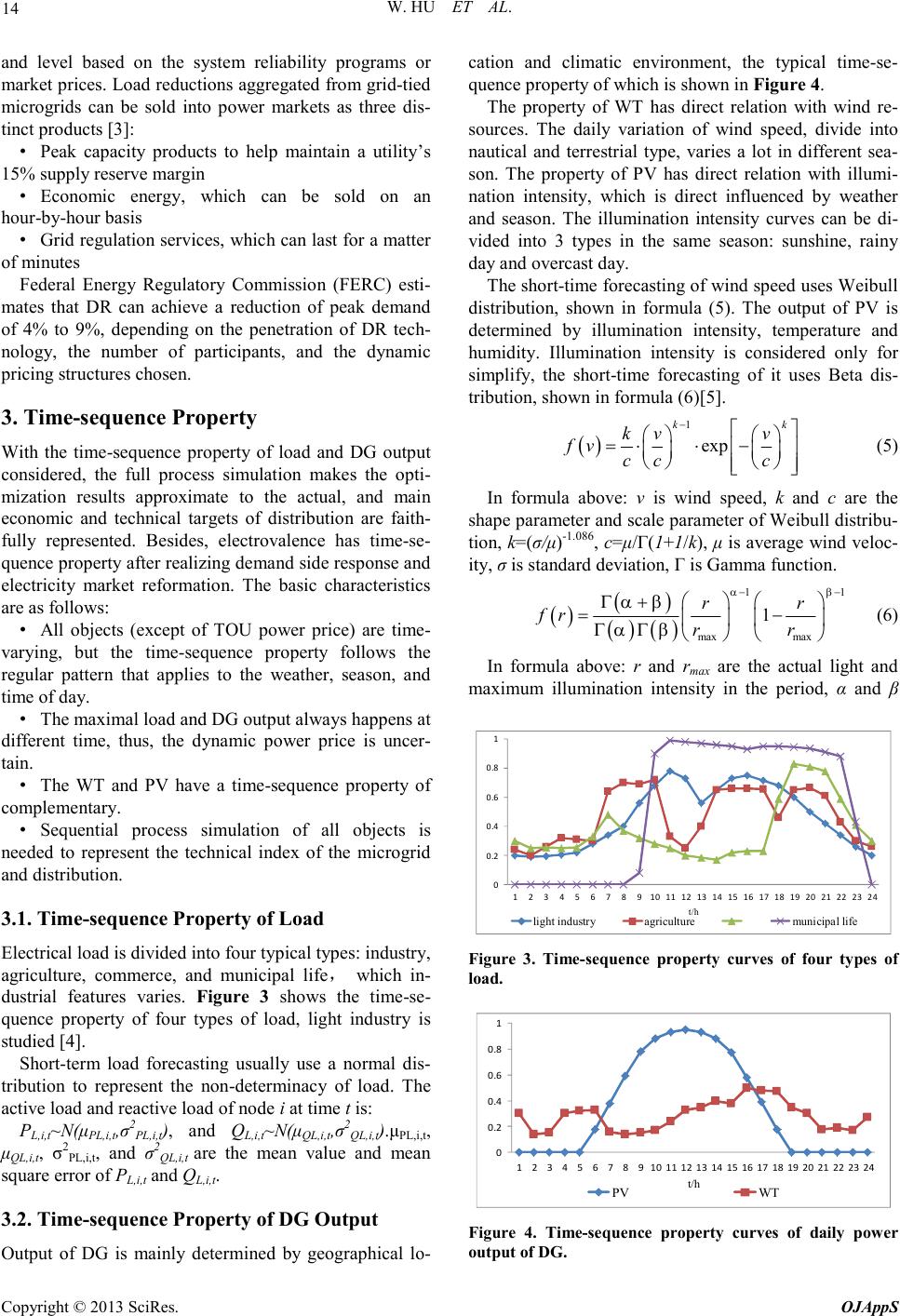

W. HU ET AL.

and level based on the system reliability programs or

market prices. Load reductions aggregated from grid-tied

microgrids can be sold into power markets as three dis-

tinct products [3]:

• Peak capacity products to help maintain a utility’s

15% supply reserve margin

• Economic energy, which can be sold on an

hour-by-hour basis

• Grid regulation services, which can last for a matter

of minutes

Federal Energy Regulatory Commission (FERC) esti-

mates that DR can achieve a reduction of peak demand

of 4% to 9%, depending on the penetration of DR tech-

nology, the number of participants, and the dynamic

pricing structures chosen.

3. Time-sequence Property

With the time-sequence property of load and DG output

considered, the full process simulation makes the opti-

mization results approximate to the actual, and main

economic and technical targets of distribution are faith-

fully represented. Besides, electrovalence has time-se-

quence property after realizing demand side response and

electricity market reformation. The basic characteristics

are as follows:

• All objects (except of TOU power price) are time-

varying, but the time-sequence property follows the

regular pattern that applies to the weather, season, and

time of day.

• The maximal load and DG output always happens at

different time, thus, the dynamic power price is uncer-

tain.

• The WT and PV have a time-sequence property of

complementary.

• Sequential process simulation of all objects is

needed to represent the technical index of the microgrid

and distribution.

3.1. Time-sequence Property of Load

Electrical load is divided into four typical types: industry,

agriculture, commerce, and municipal life ， which in-

dustrial features varies. Figure 3 shows the time-se-

quence property of four types of load, light industry is

studied [4].

Short-term load forecasting usually use a normal dis-

tribution to represent the non-determinacy of load. The

active load and reactive load of node i at time t is:

PL,i,t~N(μPL,i,t,σ2PL,i,t), and QL,i,t~N(μQL,i,t,σ2QL,i,t).μPL,i,t,

μQL,i,t, σ2PL,i,t, and σ2QL,i,t are the mean value and mean

square error of PL,i,t and QL,i,t.

3.2. Time-sequence Property of DG Output

Output of DG is mainly determined by geographical lo-

cation and climatic environment, the typical time-se-

quence property of which is shown in Figure 4.

The property of WT has direct relation with wind re-

sources. The daily variation of wind speed, divide into

nautical and terrestrial type, varies a lot in different sea-

son. The property of PV has direct relation with illumi-

nation intensity, which is direct influenced by weather

and season. The illumination intensity curves can be di-

vided into 3 types in the same season: sunshine, rainy

day and overcast day.

The short-time forecasting of wind speed uses Weibull

distribution, shown in formula (5). The output of PV is

determined by illumination intensity, temperature and

humidity. Illumination intensity is considered only for

simplify, the short-time forecasting of it uses Beta dis-

tribution, shown in formula (6)[5].

()

exp

kvv

fv ccc

−





=⋅⋅−











(5)

In formula above: v is wind speed, k and c are the

shape parameter and scale parameter of Weibull distribu-

tion, k=(σ/μ)-1.086, c=μ/Γ(1+1/k), μ is average wind veloc-

ity, σ is standard deviation, Γ is Gamma function.

() ( )

maxmax

fr rr

αβ

−−

Γ+



=−



ΓΓ



(6)

In formula above: r and rmax are the actual light and

maximum illumination intensity in the period, α and β

0.2

0.4

0.6

0.8

1 2 3 4 56 7 8 9101112131415161718192021222324

t/h

light industry agriculture municipal life

Figure 3. Time-sequence property curves of four types of

load.

0.2

0.4

0.6

0.8

123456789101112131415161718192021222324

t/h

PV WT

Figure 4. Time-sequence property curves of daily power

output of DG.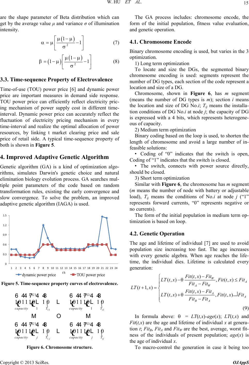

W. HU ET AL.

are the shape parameter of Beta distribution which can

get by the average value μ and variance σ of illumination

intensity.

(

)

µµ

αµ σ

−



=−





(7)

( )

(

)

µµ

βµ

−



=−−





(8)

3.3. Time-sequence Property of Electrovalence

Time-of-use (TOU) power price [6] and dynamic power

price are important measures in demand side response.

TOU power price can efficiently reflect electricity pric-

ing mechanism of power supply cost in different time-

interval. Dynamic power price can accurately reflect the

fluctuation of electricity pricing mechanism in every

time-interval and realize the optimal allocation of power

resources, by linking t market clearing price and sale

price of retail side. A typical time-sequence property of

both is shown in Figure 5.

4. Improved Adaptive Genetic Algorithm

Genetic algorithm (GA) is a kind of optimization algo-

rithms, simulates Darwin's genetic choice and natural

elimination biology evolution process. GA searches mul-

tiple point parameters of the code based on random

transformation rules, existing the early convergence and

slow convergence. To solve the problem, an improved

adaptive genetic algorithm (IAGA) is used.

0.3

0.6

0.9

1.2

1.5

123456789101112131415161718192021222324

t/h

dynamic power price TOU power price

Figure 5. Time-sequence property curves of electrovalence.

{

111

1011101010111010

jij

DGDGi

capacityTcapacityT

DGDGi

capacityjTcapacityjT

64474486447448

LLL

MOM

64474486447448

LLL

Figure 6. Chromosome structure.

The GA process includes: chromosome encode, the

form of the initial population, fitness value evaluation,

and genetic operation.

4.1. Chromosome Encode

Binary chromosome encoding is used, but varies in the 3

optimization.

1) Long term optimization

To locate and size the DGs, the segmented binary

chromosome encoding is used: segments represent the

number of DG types, each section of the code represent a

location and size of a DG.

Chromosome, shown in Figure 6, has m segment

(means the number of DG types is m); section i means

the location and size of DG No.i; Tij means the installa-

tion conditions of DG No.i at node j; the capacity of DG

is expressed with a 4 bits, which represents heterogene-

ous of capacity.

2) Medium term optimization

Binary coding based on the loop is used, to shorten the

length of chromosome and avoid a large number of in-

feasible solutions:

• Coding of “0” indicates that the switch is open,

Coding of “1” indicates that the switch is closed.

• The switch, connects with power source directly,

should be closed.

3) Short term optimization

Similar with Figure 6, the chromosome has m segment

(m means the number of node with battery or adjustable

load), Tij means the conditions of No.i at node j (“1”

represents forward currents, “0” represents negative or

no currents).

The form of the initial population in medium term op-

timization is based on loop.

4.2. Genetic Operation

The age and lifetime of individual [7] are used to avoid

population size increasing too fast. The age increases

with every genetic algebra. When age reaches the life-

time, the individual dies. Lifetime is calculated every

generation:

(,)

(,),(,)

(1,) (,)

(,),(,)

FittxFit

LTtxFittxFit

FitFit

LTtx FittxFit

LTtxFittxFit

FitFit

−

−≤



−



−

+

−





(9)

In formula above:

= LT(t,x)-age(x); LT(t,x) and

Fit(t,x) are the age and lifetime of individual x at genera-

tion t; FitB, FitA and FitW are the best, average, worst fit-

ness of the individuals of present population; age(x) is

the age of individual x.

To macro-control the generation in case it being too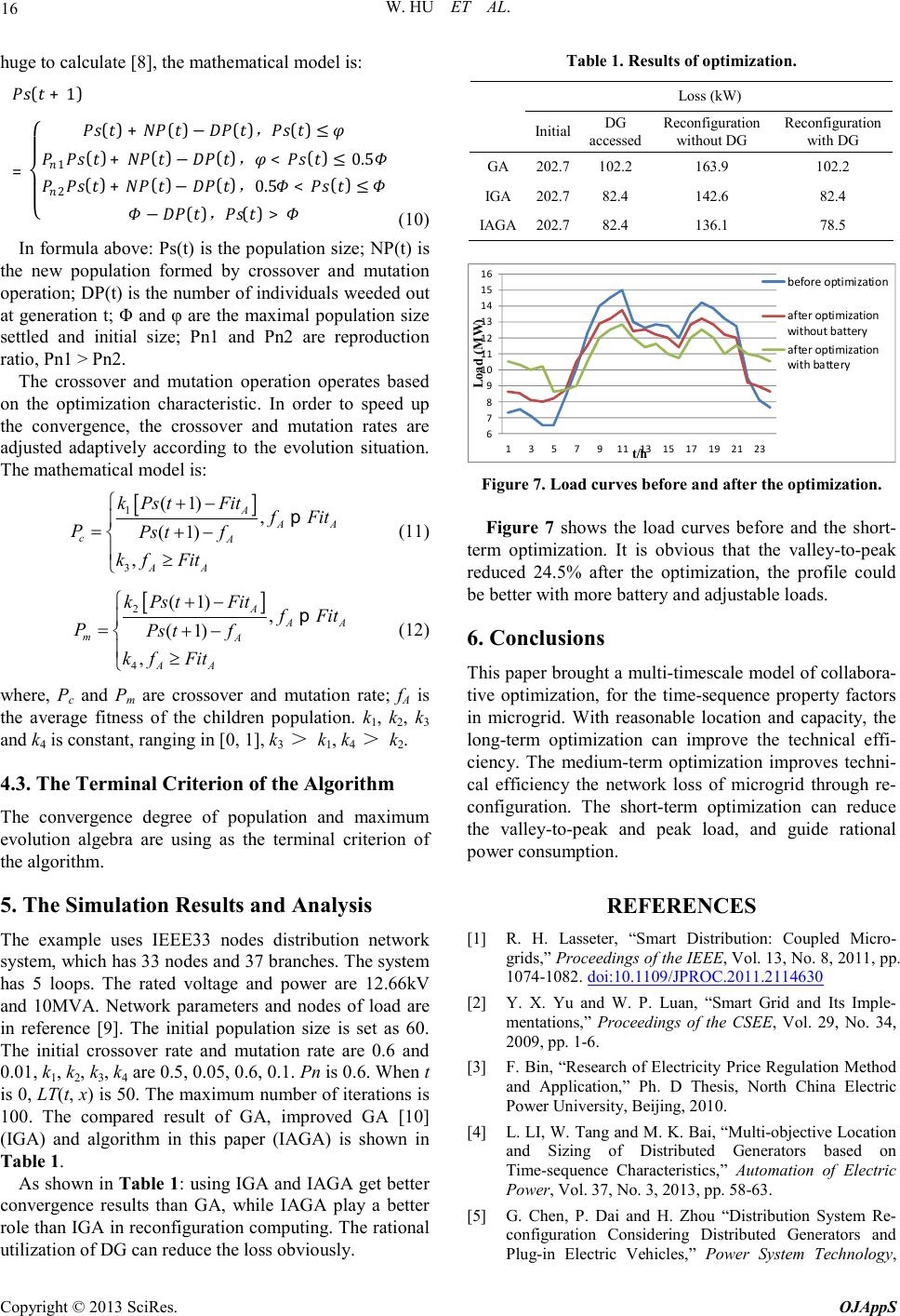

W. HU ET AL.

huge to calculate [8], the mathematical model is:

(

)

'(())+*+(,)-./(0)

，

12(3)45

67189(:)+;<(=)->?(@)

，

A<BC(D)40.5E

(

)

(

)

(

)

，

(

)

(

)

，

(

)

]

(10)

In formula above: Ps(t) is the population size; NP(t) is

the new population formed by crossover and mutation

operation; DP(t) is the number of individuals weeded out

at generation t; Φ and φ are the maximal population size

settled and initial size; Pn1 and Pn2 are reproduction

ratio, Pn1 > Pn2.

The crossover and mutation operation operates based

on the optimization characteristic. In order to speed up

the convergence, the crossover and mutation rates are

adjusted adaptively according to the evolution situation.

The mathematical model is:

[

]

(1) ,

(1)

kPstFit

fFit

PPstf

kfFit

+−



=+−



≥



p (11)

[

]

(1) ,

(1)

kPstFit

fFit

PPstf

kfFit

+−



=+−



≥



p (12)

where, Pc and Pm are crossover and mutation rate; fA is

the average fitness of the children population. k1, k2, k3

and k4 is constant, ranging in [0, 1], k3 ＞ k1, k4 ＞ k2.

4.3. The Terminal Criterion of the Algorithm

The convergence degree of population and maximum

evolution algebra are using as the terminal criterion of

the algorithm.

5. The Simulation Results and Analysis

The example uses IEEE33 nodes distribution network

system, which has 33 nodes and 37 branches. The system

has 5 loops. The rated voltage and power are 12.66kV

and 10MVA. Network parameters and nodes of load are

in reference [9]. The initial population size is set as 60.

The initial crossover rate and mutation rate are 0.6 and

0.01, k1 , k2, k3, k4 are 0.5, 0.05, 0.6, 0.1. Pn is 0.6. When t

is 0, LT(t, x) is 50. The maximum number of iterations is

100. The compared result of GA, improved GA [10]

(IGA) and algorithm in this paper (IAGA) is shown in

Table 1.

As shown in Table 1: using IGA and IAGA get better

convergence results than GA, while IAGA play a better

role than IGA in reconfiguration computing. The rational

utilization of DG can reduce the loss obviously.

Table 1. Results of optimization.

Loss (kW)

Initial

accessed

Reconfiguration

without DG Reconfiguration

with DG

GA 202.7

102.2 163.9 102.2

IGA

202.7

82.4 142.6 82.4

IAGA

202.7

82.4 136.1 78.5

1 3 5 7 91113 15 17 19 21 23

Load (MW)

t/h

before optimization

after optimization

without battery

after optimization

with battery

Figure 7. Load curves before and after the optimization.

Figure 7 shows the load curves before and the short-

term optimization. It is obvious that the valley-to-peak

reduced 24.5% after the optimization, the profile could

be better with more battery and adjustable loads.

6. Conclusions

This paper brought a multi-timescale model of collabora-

tive optimization, for the time-sequence property factors

in microgrid. With reasonable location and capacity, the

long-term optimization can improve the technical effi-

ciency. The medium-term optimization improves techni-

cal efficiency the network loss of microgrid through re-

configuration. The short-term optimization can reduce

the valley-to-peak and peak load, and guide rational

power consumption.

REFERENCES

[1] R. H. Lasseter, “Smart Distribution: Coupled Micro-

grids,” Proceedings of the IEEE, Vol. 13, No. 8, 2011, pp.

1074-1082. doi:10.1109/JPROC.2011.2114630

[2] Y. X. Yu and W. P. Luan, “Smart Grid and Its Imple-

mentations,” Proceedings of the CSEE, Vol. 29, No. 34,

2009, pp. 1-6.

[3] F. Bin, “Research of Electricity Price Regulation Method

and Application,” Ph. D Thesis, North China Electric

Power University, Beijing, 2010.

[4] L. LI, W. Tang and M. K. Bai, “Multi-objective Location

and Sizing of Distributed Generators based on

Time-sequence Characteristics,” Automation of Electric

Power, Vol. 37, No. 3, 2013, pp. 58-63.

[5] G. Chen, P. Dai and H. Zhou “Distribution System Re-

configuration Considering Distributed Generators and

Plug-in Electric Vehicles,” Power System Technology,

W. HU ET AL.

Vol. 37, No. 1, 2013, pp. 82-88.

[6] J. Li, J. Y. Liu, L. F. Xie, H. Quan and Y. B. Liu, “Dy-

namic Game Linkage of TOU Pricing Between Generat-

ing Side and Retail Side,” Electric Power Automation

Equipment, Vol. 32, No. 4, 2012, pp. 16-19.

[7] J. Arabas，Z. Michalewicz and J. Mulawka, “GAVaPS：

A Genetic Algorithm with Varying Population Size,”

Proceedings of the 1st IEEE Conference on Evolutionary

Computation, 1994, pp. 73-78.

[8] X. Jin, “The Application of Genetic Algorithm with

Adaptive Population Size in Distribution Network,”

North China Electric Power University, Beijing, 2011.

[9] H. Zhang, “Study of Distribution Network Fault Restora-

tion Based on Genetic and Particle Swarm Mixed Algo-

rithm,” Wuhan University, Wuhan, 2009.

[10] S. Q. Sheng, Z. G. Ma and J. Wu, “Distribution Network

Fault Restoration Based on Improved Adaptive Genetic

Algorithm,” Second Conference on Intelligent Computa-

tion Technology and Automation, 2009.