 Applied Mathematics, 2013, 4, 1392-1396 http://dx.doi.org/10.4236/am.2013.410188 Published Online October 2013 (http://www.scirp.org/journal/am) Copyright © 2013 SciRes. AM In-Place Matrix Inversion by Modified Gauss-Jordan Algorithm Debabrata DasGupta 1,2,3* 1 (Former) LEAP Software, Inc., Tampa, FL, USA 2 (Former) McDonnell Douglas Automation Co., St., Louis, MO, USA 3 (Former) Central Water and Power Commission, New Delhi, India Email: DDasGupta@email.com Received July 30, 2013; revised August 30, 2013; accepted September 7, 2013 Copyright © 2013 Debabrata DasGupta. This is an open access article distributed under the Creative Commons Attribution License, which permits unrestricted use, distribution, and reproduction in any medium, provided the original work is properly cited. ABSTRACT The classical Gauss-Jordan method for matrix inversion involves augmenting the matrix with a unit matrix and requires a workspace twice as large as the original matrix as well as computational operations to be performed on both the orig- inal and the unit matrix. A modified version of the method for performing the inversion without explicitly generating the unit matrix by replicating its functionality within the original matrix space for more efficient utilization of computa- tional resources is presented in this article. Although the algorithm described here picks the pivots solely from the di- agonal which, therefore, may not contain a zero, it did not pose any problem for the author because he used it to invert structural stiffness matrices which met this requirement. Techniques such as row/column swapping to handle off-di- agonal pivots are also applicable to this method but are beyond the scope of this article. Keywords: Numerical Methods; Gauss-Jordan; Matrices; Inversion; In-Place; In-Core; Structural Analysis 1. Introduction Gauss-Jordan [1] is a standard matrix inversion proce- dure developed in 1887. It requires the original matrix to be appended by a unit (identity) matrix and after the in- version operation is completed the original matrix is transformed into a unit matrix while the appended unit matrix becomes the inverse. During the early days of his career as a professional engineer and software developer [2], the author created an engineering software library for the Government of India in the mid-1960s. Some of the softwares were in the field of structural analysis which involved computing displacement vectors for multiple load vectors applied to the same stiffness matrix created using the modeling tech- nique suggested by Tezcan [3]. Since his work involved handling large numbers of loading cases applied to the same structure, he opted for matrix inversion to generate flexibility matrices instead of solution of equations to process the load vectors be- cause the latter method would require either regeneration or retrieval of the stiffness matrix to process every load vector, either of which would substantially increase the computational time and effort. 2. Development The stiffness matrices encountered in structural analysis have three important characteristics. Their largest ele- ments always fall on the diagonal which can never have a zero element and they are always symmetrical. The au- thor started with the Gauss-Jordan algorithm however, since both computing power and hardware speed were severely limited in those days, he attempted to carry out as much of his work within the computer memory (in- core) as possible. Since Gauss-Jordan required an aug- menting unit matrix and therefore both memory space and amount of computation for a matrix twice as large as the original matrix, he sought a way around this problem. Since after a pivotal column of the original matrix is processed with the Gauss-Jordan method, it always con- tains a unity (1) on the diagonal and zeroes in all other rows and remains unchanged during all subsequent oper- ations without any mathematical utility, the author felt that this memory space could be utilized to replicate the corresponding column of a virtual unit matrix without creating a real unit matrix. He used this idea to develop a modified procedure to simulate a non-existent augment- ing unit matrix and called it virtualization of the aug- M. Tech., P.E., M.ASCE, MCP. 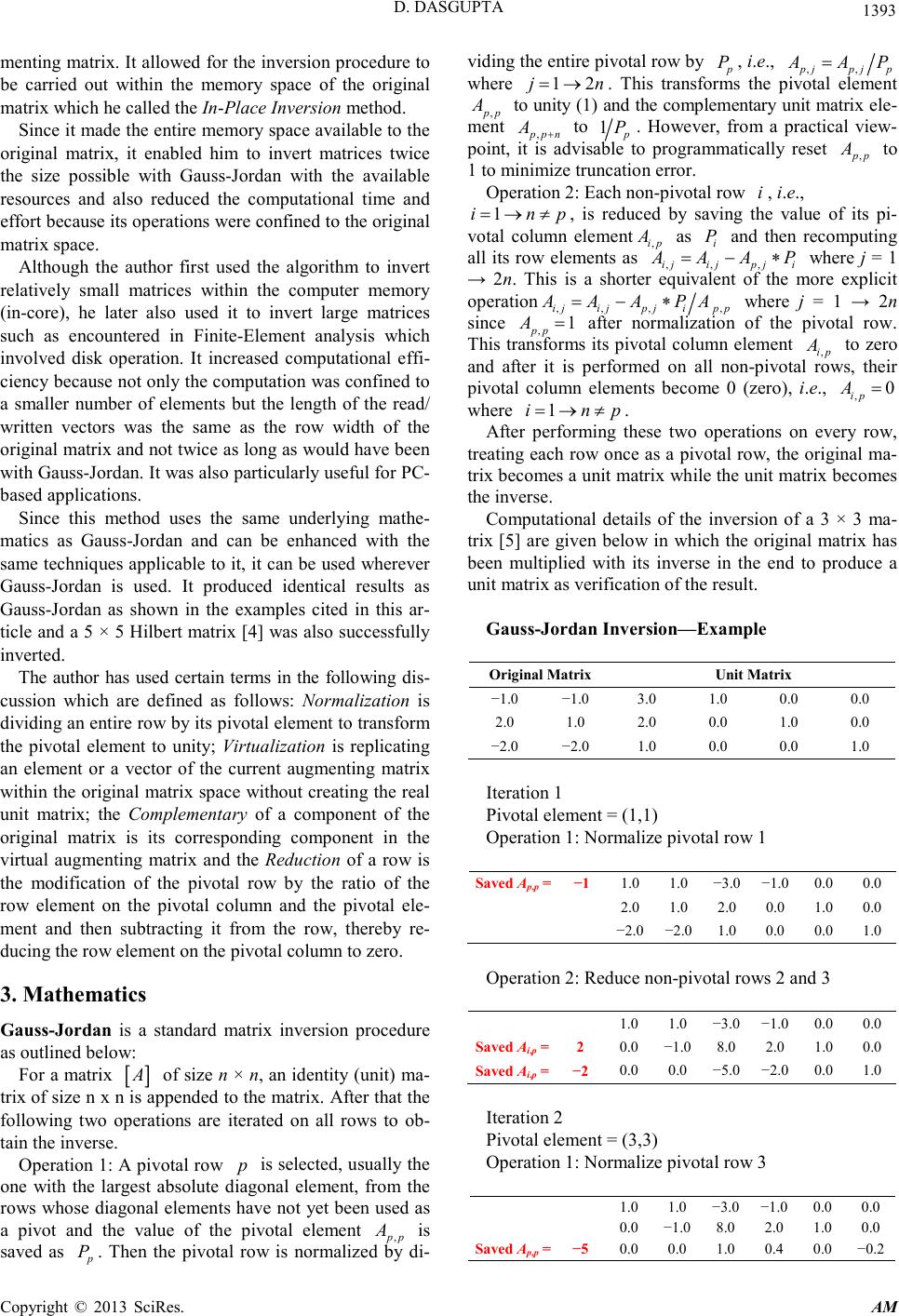 D. DASGUPTA Copyright © 2013 SciRes. AM menting matrix. It allowed for the inversion procedure to be carried out within the memory space of the original matrix which he called the In-Place Inversion method. Since it made the entire memory space available to the original matrix, it enabled him to invert matrices twice the size possible with Gauss-Jordan with the available resources and also reduced the computational time and effort because its operations were confined to the original matrix space. Although the author first used the algorithm to invert relatively small matrices within the computer memory (in-core), he later also used it to invert large matrices such as encountered in Finite-Element analysis which involved disk operation. It increased computational effi- ciency because not only the computation was confined to a smaller number of elements but the length of the read/ written vectors was the same as the row width of the original matrix and not twice as long as would have been with Gauss-Jordan. It was also particularly useful for PC- based applications. Since this method uses the same underlying mathe- matics as Gauss-Jordan and can be enhanced with the same techniques applicable to it, it can be used wherever Gauss-Jordan is used. It produced identical results as Gauss-Jordan as shown in the examples cited in this ar- ticle and a 5 × 5 Hilbert matrix [4] was also successfully inverted. The author has used certain terms in the following dis- cussion which are defined as follows: Normalization is dividing an entire row by its pivotal element to transform the pivotal element to unity; Virtualization is replicating an element or a vector of the current augmenting matrix within the original matrix space without creating the real unit matrix; the Complementary of a component of the original matrix is its corresponding component in the virtual augmenting matrix and the Reduction of a row is the modification of the pivotal row by the ratio of the row element on the pivotal column and the pivotal ele- ment and then subtracting it from the row, thereby re- ducing the row element on the pivotal column to zero. 3. Mathematics Gauss-Jordan is a standard matrix inversion procedure as outlined below: For a matrix of size n × n, an identity (unit) ma- trix of size n x n is appended to the matrix. After that the following two operations are iterated on all rows to ob- tain the inverse. Operation 1: A pivotal row is selected, usually the one with the largest absolute diagonal element, from the rows whose diagonal elements have not yet been used as a pivot and the value of the pivotal element is saved as . Then the pivotal row is normalized by di- viding the entire pivotal row by , i.e., where . This transforms the pivotal element to unity (1) and the complementary unit matrix ele- ment , + to . However, from a practical view- point, it is advisable to programmatically reset to 1 to minimize truncation error. Operation 2: Each non-pivotal row , i.e., , is reduced by saving the value of its pi- votal column element as and then recomputing all its row elements as where j = 1 → 2n. This is a shorter equivalent of the more explicit operation where j = 1 → 2n since after normalization of the pivotal row. This transforms its pivotal column element to zero and after it is performed on all non-pivotal rows, their pivotal column elements become 0 (zero), i.e., where . After performing these two operations on every row, treating each row once as a pivotal row, the original ma- trix becomes a unit matrix while the unit matrix becomes the inverse. Computational details of the inversion of a 3 × 3 ma- trix [5] are given below in which the original matrix has been multiplied with its inverse in the end to produce a unit matrix as verification of the result. Gauss-Jordan Inversion—Example −1.0 −1.0 3.0 1.0 0.0 0.0 2.0 1.0 2.0 0.0 1.0 0.0 −2.0 −2.0 1.0 0.0 0.0 1.0 Iteration 1 Pivotal element = (1,1) Operation 1: Normalize pivotal row 1 Saved A p,p = −1 1.0 1.0 −3.0 −1.0 0.0 0.0 −2.0 −2.0 1.0 0.0 0.0 1.0 Operation 2: Reduce non-pivotal rows 2 and 3 1.0 1.0 −3.0 −1.0 0.0 0.0 Saved A i,p = 2 0.0 −1.0 8.0 2.0 1.0 0.0 i,p Iteration 2 Pivotal element = (3,3) Operation 1: Normalize pivotal row 3 1.0 1.0 −3.0 −1.0 0.0 0.0 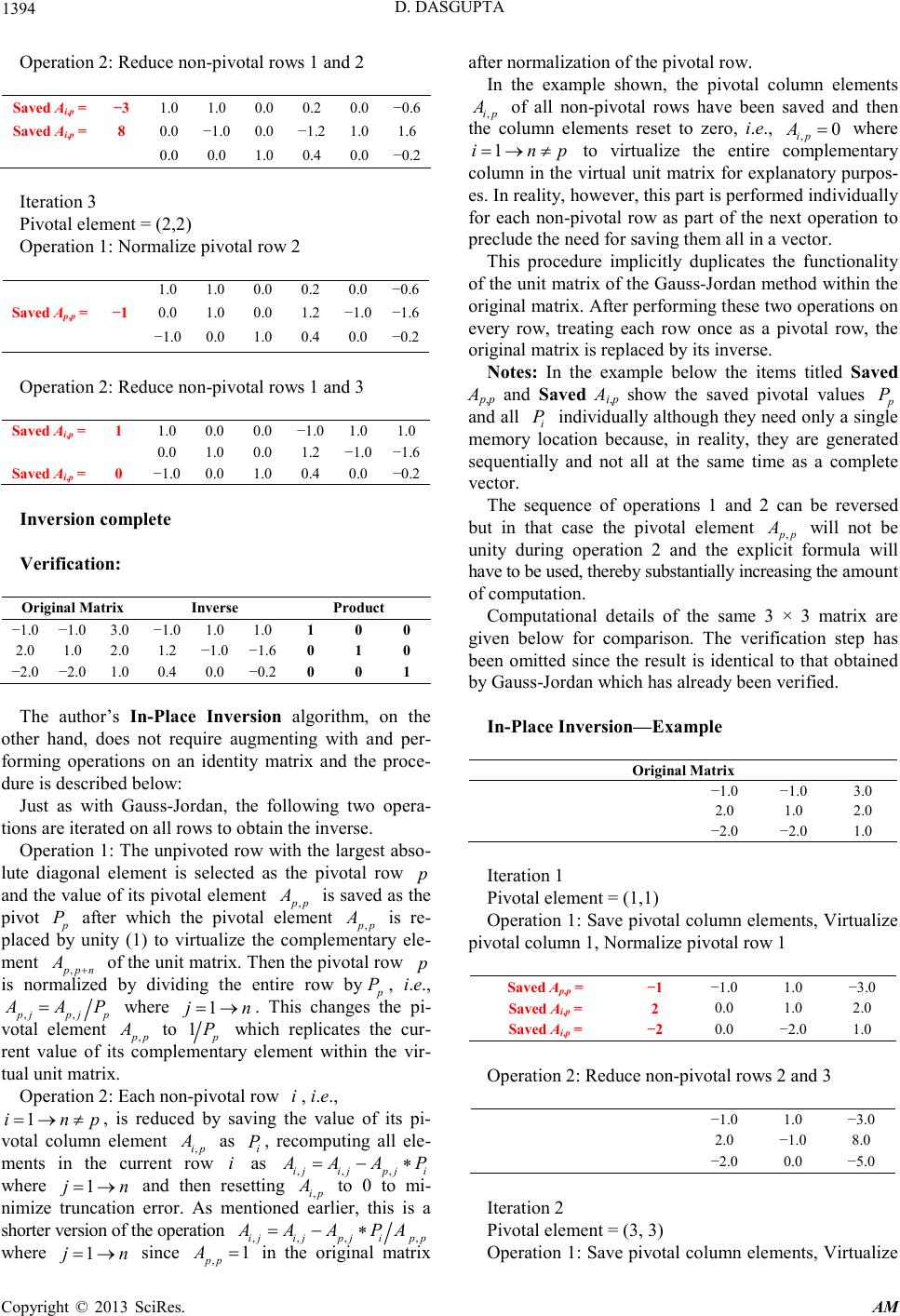 D. DASGUPTA Copyright © 2013 SciRes. AM Operation 2: Reduce non-pivotal rows 1 and 2 Saved A i,p = −3 1.0 1.0 0.0 0.2 0.0 −0.6 Saved A i,p = 8 0.0 −1.0 0.0 −1.2 1.0 1.6 Iteration 3 Pivotal element = (2,2) Operation 1: Normalize pivotal row 2 p,p Operation 2: Reduce non-pivotal rows 1 and 3 i,p i,p Inversion complete Verification: The author’s In-Place Inversion algorithm, on the other hand, does not require augmenting with and per- forming operations on an identity matrix and the proce- dure is described below: Just as with Gauss-Jordan, the following two opera- tions are iterated on all rows to obtain the inverse. Operation 1: The unpivoted row with the largest abso- lute diagonal element is selected as the pivotal row and the value of its pivotal element is saved as the pivot after which the pivotal element is re- placed by unity (1) to virtualize the complementary ele- ment of the unit matrix. Then the pivotal row is normalized by dividing the entire row by , i.e., where . This changes the pi- votal element to which replicates the cur- rent value of its complementary element within the vir- tual unit matrix. Operation 2: Each non-pivotal row , i.e., , is reduced by saving the value of its pi- votal column element as , recomputing all ele- ments in the current row as where and then resetting to 0 to mi- nimize truncation error. As mentioned earlier, this is a shorter version of the operation where since in the original matrix after normalization of the pivotal row. In the example shown, the pivotal column elements of all non-pivotal rows have been saved and then the column elements reset to zero, i.e., where to virtualize the entire complementary column in the virtual unit matrix for explanatory purpos- es. In reality, however, this part is performed individually for each non-pivotal row as part of the next operation to preclude the need for saving them all in a vector. This procedure implicitly duplicates the functionality of the unit matrix of the Gauss-Jordan method within the original matrix. After performing these two operations on every row, treating each row once as a pivotal row, the original matrix is replaced by its inverse. Notes: In the example below the items titled Saved A p,p and Saved A i,p show the saved pivotal values and all individually although they need only a single memory location because, in reality, they are generated sequentially and not all at the same time as a complete vector. The sequence of operations 1 and 2 can be reversed but in that case the pivotal element will not be unity during operation 2 and the explicit formula will have to be used, thereby substantially increasing the amount of computation. Computational details of the same 3 × 3 matrix are given below for comparison. The verification step has been omitted since the result is identical to that obtained by Gauss-Jordan which has already been verified. In-Place Inversion—Example Iteration 1 Pivotal element = (1,1) Operation 1: Save pivotal column elements, Virtualize pivotal column 1, Normalize pivotal row 1 Saved p,p = −1 −1.0 1.0 −3.0 Operation 2: Reduce non-pivotal rows 2 and 3 −1.0 1.0 −3.0 Iteration 2 Pivotal element = (3, 3) Operation 1: Save pivotal column elements, Virtualize 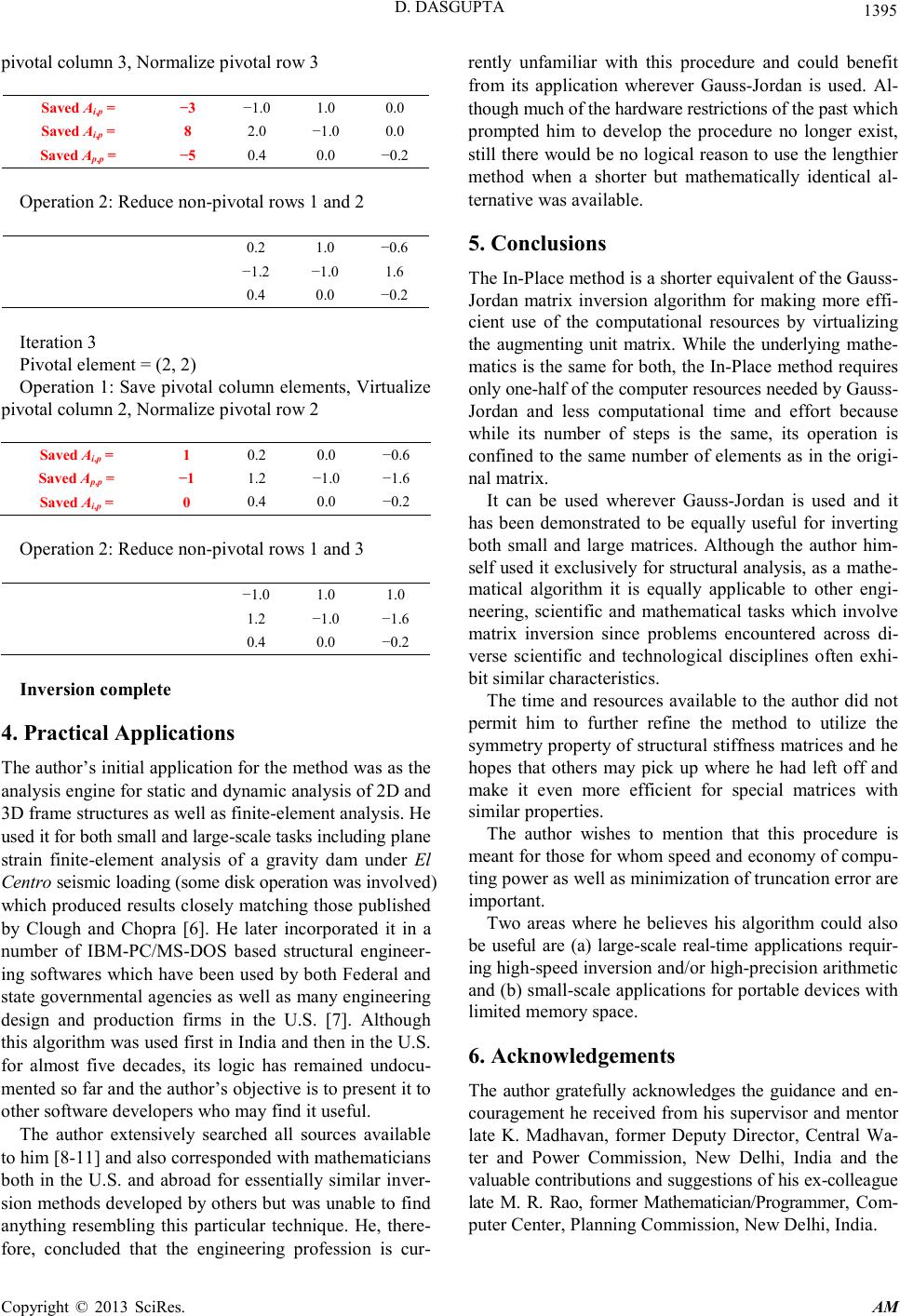 D. DASGUPTA Copyright © 2013 SciRes. AM pivotal column 3, Normalize pivotal row 3 Saved A i,p = −3 −1.0 1.0 0.0 Saved A i,p = 8 2.0 −1.0 0.0 p,p Operation 2: Reduce non-pivotal rows 1 and 2 0.2 1.0 −0.6 −1.2 −1.0 1.6 0.4 0.0 −0.2 Iteration 3 Pivotal element = (2, 2) Operation 1: Save pivotal column elements, Virtualize pivotal column 2, Normalize pivotal row 2 i,p Saved A p,p = −1 1.2 −1.0 −1.6 Saved A i,p = 0 0.4 0.0 −0.2 Operation 2: Reduce non-pivotal rows 1 and 3 −1.0 1.0 1.0 0.4 0.0 −0.2 Inversion complete 4. Practical Applications The author’s initial application for the method was as the analysis engine for static and dynamic analysis of 2D and 3D frame structures as well as finite-element analysis. He used it for both small and large-scale tasks including plane strain finite-element analysis of a gravity dam under El Centro seismic loading (some disk operation was involved) which produced results closely matching those published by Clough and Chopra [6]. He later incorporated it in a number of IBM-PC/MS-DOS based structural engineer- ing softwares which have been used by both Federal and state governmental agencies as well as many engineering design and production firms in the U.S. [7]. Although this algorithm was used first in India and then in the U.S. for almost five decades, its logic has remained undocu- mented so far and the author’s objective is to present it to other software developers who may find it useful. The author extensively searched all sources available to him [8-11] and also corresponded with mathematicians both in the U.S. and abroad for essentially similar inver- sion methods developed by others but was unable to find anything resembling this particular technique. He, there- fore, concluded that the engineering profession is cur- rently unfamiliar with this procedure and could benefit from its application wherever Gauss-Jordan is used. Al- though much of the hardware restrictions of the past which prompted him to develop the procedure no longer exist, still there would be no logical reason to use the lengthier method when a shorter but mathematically identical al- ternative was available. 5. Conclusions The In-Place method is a shorter equivalent of the Gauss- Jordan matrix inversion algorithm for making more effi- cient use of the computational resources by virtualizing the augmenting unit matrix. While the underlying mathe- matics is the same for both, the In-Place method requires only one-half of the computer resources needed by Gauss- Jordan and less computational time and effort because while its number of steps is the same, its operation is confined to the same number of elements as in the origi- nal matrix. It can be used wherever Gauss-Jordan is used and it has been demonstrated to be equally useful for inverting both small and large matrices. Although the author him- self used it exclusively for structural analysis, as a mathe- matical algorithm it is equally applicable to other engi- neering, scientific and mathematical tasks which involve matrix inversion since problems encountered across di- verse scientific and technological disciplines often exhi- bit similar characteristics. The time and resources available to the author did not permit him to further refine the method to utilize the symmetry property of structural stiffness matrices and he hopes that others may pick up where he had left off and make it even more efficient for special matrices with similar properties. The author wishes to mention that this procedure is meant for those for whom speed and economy of compu- ting power as well as minimization of truncation error are important. Two areas where he believes his algorithm could also be useful are (a) large-scale real-time applications requir- ing high-speed inversion and/or high-precision arithmetic and (b) small-scale applications for portable devices with limited memory space. 6. Acknowledgements The author gratefully acknowledges the guidance and en- couragement he received from his supervisor and mentor late K. Madhavan, former Deputy Director, Central Wa- ter and Power Commission, New Delhi, India and the valuable contributions and suggestions of his ex-colleague late M. R. Rao, former Mathematician/Programmer, Com- puter Center, Planning Commission, New Delhi, India.  D. DASGUPTA Copyright © 2013 SciRes. AM REFERENCES [1] W. A. Smith, “Elementary Numerical Analysis,” Pren- tice-Hall, Inc., Englewood Cliffs, 1986, pp. 51-52. [2] D. DasGupta, “McAuto STRUDL RECON—A Rein- forced Concrete Frame Design Software,” Concrete In- ternational, Nov 1982, pp. 37-42. http://www.concreteinternational.com/pages/featured_arti cle.asp?ID=9129 [3] S. S. Tezcan, “Discussion,” Journal of the Structural Division, American Society of Civil Engineers, Vol. 89, No. ST6, Part I, 1963, p. 445. [4] J. H. Mathews, “Lab for Matrix Inversion, Exercise 2,” California State University, Fullerton, 1998. http://math.fullerton.edu/mathews/numerical/mi.htm [5] T. McFarland, “The Inverse of an n × n Matrix,” Univer- sity of Wisconsin-Whitewater, Whitewater, 2007. http://math.uww.edu/faculty/mcfarlat/inverse.htm [6] R. W. Clough and A. K Chopra, “Earthquake Stress Analysis in Earth Dams,” University of California, Berkeley, 1965, 24p. [7] Staff Reporter, “Roads, Bridges and Computers,” Roads & Bridges Magazine, May 1987, p. 48. [8] V. A. Patel, “Numerical Analysis,” Harcourt Brace Col- lege Publishers, Fort Worth, 1994, pp. 216-218. [9] B. Noble, “Applied Linear Algebra,” Prentice-Hall, Inc., Englewood Cliffs, 1969, pp. 214-215. [10] G. Mills, “Introduction to Linear Algebra for Social Scientists,” George Allen and Unwin, Ltd., London, 1969, pp. 104-105. [11] R. H. Pennington, “Introductory Computer Methods and Numerical Analysis,” The McMillan Co., New York, 1968, pp. 323-325.
|