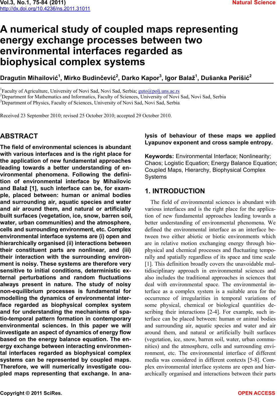
Vol.3, No.1, 75-84 (2011) Natural Science
http://dx.doi.org/10.4236/ns.2011.31011
A numerical study of coupled maps representing
energy exchange processes between two
environmental interfaces regarded as
biophysical complex systems
Dragutin Mihailović1, Mirko Budinčević2, Darko Kapor3, Igor Balaž1, Dušanka Perišić2
1Faculty of Agriculture, University of Novi Sad, Novi Sad, Serbia;
2Department for Mathematics and Informatics, Faculty of Sciences, University of Novi Sad, Novi Sad, Serbia
3Department of Physics, Faculty of Sciences, University of Novi Sad, Novi Sad, Serbia
Received 23 September 2010; revised 25 October 2010; accepted 29 October 2010.
ABSTRACT
The field of environmental sciences is abundant
with various interfaces and is the right place for
the application of new fundamental approaches
leading towards a better understanding of en-
vironmental phenomena. Following the defini-
tion of environmental interface by Mihailovic
and Balaž [1], such interface can be, for exam-
ple, placed between: human or animal bodies
and surrounding air, aquatic species and water
and air around them, and natural or artificially
built surfaces (vegetation, ice, snow, barren soil,
water, urban communities) and the atmosphere,
cells and surrounding environment, etc. Complex
environmental interface systems are (i) open and
hierarchically organised (ii) interactions between
their constituent parts are nonlinear, and (iii)
their interaction with the surrounding environ-
ment is noisy. These systems are therefore very
sensitive to initial conditions, deterministic ex-
ternal perturbations and random fluctuations
always present in nature. The study of noisy
non-equilibrium processes is fundamental for
modelling the dynamics of environmental inter-
face regarded as biophysical complex system
and for understanding the mechanisms of spa-
tio-temporal pattern formation in contemporary
environmental sciences. In this paper we will
investigate an aspect of dynamics of energy flow
based on the energy balance equation. The en-
ergy exchange between interacting environmen-
tal interfaces regarded as biophysical complex
systems can be represented by coupled maps.
Therefore, we will numerically investigate cou-
pled maps representing that exchange. In ana-
lysis of behaviour of these maps we applied
Lyapunov exponent and cross sample entropy.
Keywords: Environmental Interface; Nonlinearity;
Chaos; Logistic Equation; Energy Balance Equation;
Coupled Maps, Hierarchy, Biophysical Complex
Systems
1. INTRODUCTION
The field of environmental sciences is abundant with
various interfaces and is the right place for the applica-
tion of new fundamental approaches leading towards a
better understanding of environmental phenomena. We
defined the environmental interface as an interface be-
tween two either abiotic or biotic environments which
are in relative motion exchanging energy through bio-
physical and chemical processes and fluctuating tempo-
rally and spatially regardless of its space and time scale
[1]. This definition broadly covers the unavoidable mul-
tidisciplinary approach in environmental sciences and
also includes the traditional approaches in sciences that
deal with environmental space. The environmental in-
terface as a complex system is a suitable area for the
occurrence of irregularities in temporal variations of
some physical, chemical or biological quantities de-
scribing their interactions [2-4]. For example, such in-
terface can be placed between: human or animal bodies
and surrounding air, aquatic species and water and air
around them, and natural or artificially built surfaces
(vegetation, ice, snow, barren soil, water, urban commu-
nities) and the atmosphere, cells and surrounding envi-
ronment, etc. The environmental interface of different
media was considered in different contexts [5-8]. Com-
plex environmental interface systems are open and hier-
archically organised and interactions between their parts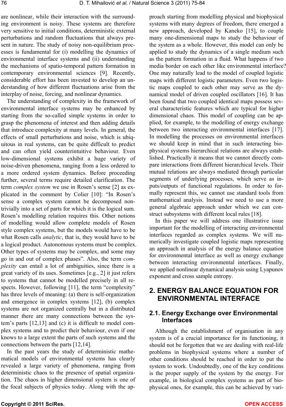

D. T. Mihailović et al. / Natural Science 3 (2011) 75-84 76
are nonlinear, while their interaction with the surround-
ing environment is noisy. These systems are therefore
very sensitive to initial conditions, deterministic external
perturbations and random fluctuations that always pre-
sent in nature. The study of noisy non-equilibrium proc-
esses is fundamental for (i) modelling the dynamics of
environmental interface systems and (ii) understanding
the mechanisms of spatio-temporal pattern formation in
contemporary environmental sciences [9]. Recently,
considerable effort has been invested to develop an un-
derstanding of how different fluctuations arise from the
interplay of noise, forcing, and nonlinear dynamics.
The understanding of complexity in the framework of
environmental interface systems may be enhanced by
starting from the so-called simple systems in order to
grasp the phenomena of interest and then adding details
that introduce complexity at many levels. In general, the
effects of small perturbations and noise, which is ubiq-
uitous in real systems, can be quite difficult to predict
and can often yield counterintuitive behaviour. Even
low-dimensional systems exhibit a huge variety of
noise-driven phenomena, ranging from a less ordered to
a more ordered system dynamics. Before proceeding
further, several terms require detailed clarification. The
term complex system we use in Rosen’s sense [2] as ex-
plicated in the comment by Colier [10]: “In Rosen’s
sense a complex system cannot be decomposed non-
trivially into a set of parts for which it is the logical sum.
Rosen’s modelling relation requires this. Other notions
of modelling would allow complete models of Rosen
style complex systems, but the models would have to be
what Rosen calls analytic, that is, they would have to be
a logical product. Autonomous systems must be complex.
Other types of systems may be complex, and some may
go in and out of complex phases”. Also, the term com-
plexity can entail a lot of ambiguities, since there is a
great variety of its uses. Sometimes [e.g., 2] it just refers
to systems that cannot be modelled precisely in all re-
spects. However, following [11], the term “complexity”
has three levels of meaning: (a) there is self-organization
and emergence in complex systems [12], (b) complex
systems are not organized centrally but in a distributed
manner there are many connections between the sys-
tem’s parts [12,13] and (c) it is difficult to model com-
plex systems and to predict their behaviour, even if one
knows to a large extent the parts of such systems and the
connections between the parts [12,14].
In the past years the study of deterministic mathe-
matical models of environmental systems has clearly
revealed a large variety of phenomena, ranging from
deterministic chaos to the presence of spatial organiza-
tion. The chaos in higher dimensional system is one of
the focal subjects of physics today. Along with the ap-
proach starting from modelling physical and biophysical
systems with many degrees of freedom, there emerged a
new approach, developed by Kaneko [15], to couple
many one-dimensional maps to study the behaviour of
the system as a whole. However, this model can only be
applied to study the dynamics of a single medium such
as the pattern formation in a fluid. What happens if two
media border on each other like environmental interface?
One may naturally lead to the model of coupled logistic
maps with different logistic parameters. Even two logis-
tic maps coupled to each other may serve as the dy-
namical model of driven coupled oscillators [16]. It has
been found that two coupled identical maps possess sev-
eral characteristic features which are typical for higher
dimensional chaos. This model of coupling can be ap-
plied, for example, to the modelling of energy exchange
between two interacting environmental interfaces [17].
In modelling the processes on environmental interfaces
we should keep in mind that in such interacting bio-
physical systems hierarchical relations are always estab-
lished. Practically it means that we cannot directly com-
pare interactions from different hierarchical levels. Their
mutual relations are always mediated through particular
segments of underlying processes, which serve as in-
puts/outputs of functional regulations. In order to for-
mally represent this, we cannot use standard tools from
mathematical analysis. Instead we need to use a more
general algebraic approach under which we can con-
struct subsystems with different local rules [18].
In this paper we will address one illustrative issue
important for the modelling of interacting environmental
interfaces regarded as complex systems. We will nu-
merically investigate coupled logistic maps representing
an approach in analysis of the energy balance equation
for environmental interface as well as energy exchange
between interacting environmental interfaces. Finally,
we applied nonlinear dynamical analysis using Lyapunov
exponent and cross sample entropy.
2. ENERGY BALANCE EQUATION FOR
ENVIRONMENTAL INTERFACE
2.1. Energy Exchange over Environmental
Interfaces
Although the establishment of organisation in any
system is of a crucial importance for its functioning, it
should not be forgotten that we are dealing with real-life
problems in biophysical systems where a number of
other conditions should be reached in order to put the
system to work. Undoubtedly, one of the key conditions
is the proper supply of the system by the energy. For
example, in biological complex systems as part of bio-
physical ones, for example, this can be achieved by vari-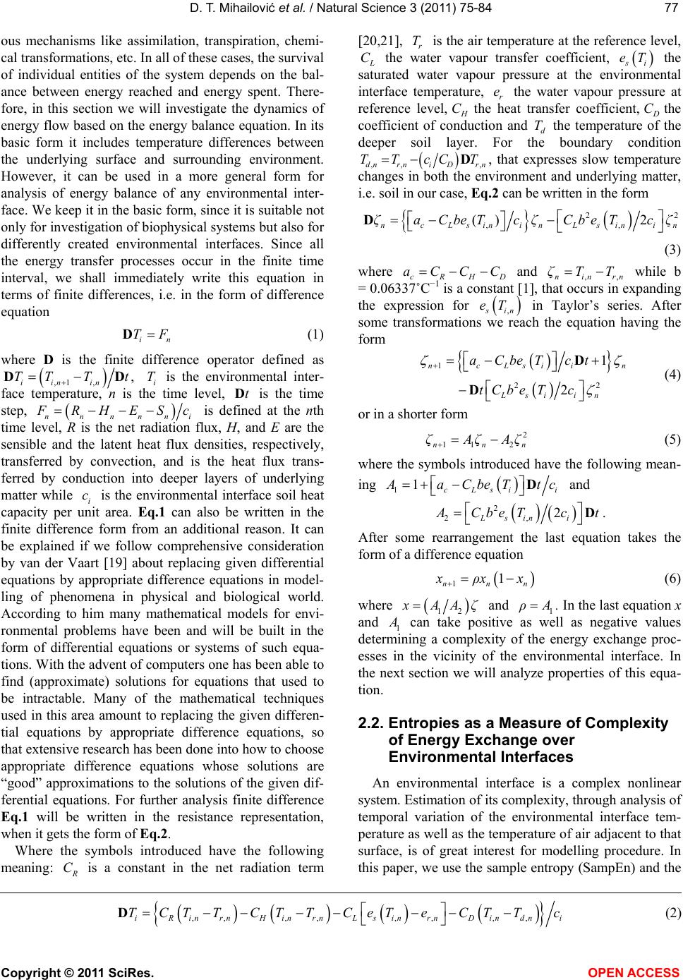

D. T. Mihailović et al. / Natural Science 3 (2011) 75-84
7777
ous mechanisms like assimilation, transpiration, chemi-
cal transformations, etc. In all of these cases, the survival
of individual entities of the system depends on the bal-
ance between energy reached and energy spent. There-
fore, in this section we will investigate the dynamics of
energy flow based on the energy balance equation. In its
basic form it includes temperature differences between
the underlying surface and surrounding environment.
However, it can be used in a more general form for
analysis of energy balance of any environmental inter-
face. We keep it in the basic form, since it is suitable not
only for investigation of biophysical systems but also for
differently created environmental interfaces. Since all
the energy transfer processes occur in the finite time
interval, we shall immediately write this equation in
terms of finite differences, i.e. in the form of difference
equation
in
TFD (1)
where D is the finite difference operator defined as

,1 ,, iin in
TT Tt

DD i T is the environmental inter-
face temperature, n is the time level, tD is the time
step,

nnnnni
F
RHES c is defined at the nth
time level, R is the net radiation flux, H, and E are the
sensible and the latent heat flux densities, respectively,
transferred by convection, and is the heat flux trans-
ferred by conduction into deeper layers of underlying
matter while i
c is the environmental interface soil heat
capacity per unit area. Eq.1 can also be written in the
finite difference form from an additional reason. It can
be explained if we follow comprehensive consideration
by van der Vaart [19] about replacing given differential
equations by appropriate difference equations in model-
ling of phenomena in physical and biological world.
According to him many mathematical models for envi-
ronmental problems have been and will be built in the
form of differential equations or systems of such equa-
tions. With the advent of computers one has been able to
find (approximate) solutions for equations that used to
be intractable. Many of the mathematical techniques
used in this area amount to replacing the given differen-
tial equations by appropriate difference equations, so
that extensive research has been done into how to choose
appropriate difference equations whose solutions are
“good” approximations to the solutions of the given dif-
ferential equations. For further analysis finite difference
Eq.1 will be written in the resistance representation,
when it gets the form of Eq.2.
Where the symbols introduced have the following
meaning:
R
C is a constant in the net radiation term
[20,21], r
T is the air temperature at the reference level,
L
C the water vapour transfer coefficient,


s
i
eT the
saturated water vapour pressure at the environmental
interface temperature, r
e the water vapour pressure at
reference level,
H
C the heat transfer coefficient,
D
C the
coefficient of conduction and d
T the temperature of the
deeper soil layer. For the boundary condition


,, ,dnrni Drn
TT cCT D, that expresses slow temperature
changes in both the environment and underlying matter,
i.e. soil in our case, Eq.2 can be written in the form



22
,,
() 2
ncLs ininLsinin
ζaCbeTcζCbeTcζ


 


D
(3)
where cRHD
aCC C

 and ,,ninrn ζTT while b
= 0.06337˚C–1 is a constant [1], that occurs in expanding
the expression for


,
s
in
eT in Taylor’s series. After
some transformations we reach the equation having the
form




1
22
1
2
ncLsii n
Lsiin
aCbeT ct
tCbe Tc



 



D
D
(4)
or in a shorter form
2
11 2nnn
ζAζAζ
 (5)
where the symbols introduced have the following mean-
ing


11cLsi i
A
aCbeT tc

 

D and



2
2,
2
Lsin i
A
CbeTct




D.
After some rearrangement the last equation takes the
form of a difference equation


11 nnn
xρ
x
x
 (6)
where


12
xAAζ and 1 ρ
A
. In the last equation x
and 1
A
can take positive as well as negative values
determining a complexity of the energy exchange proc-
esses in the vicinity of the environmental interface. In
the next section we will analyze properties of this equa-
tion.
2.2. Entropies as a Measure of Complexity
of Energy Exchange over
Environmental Interfaces
An environmental interface is a complex nonlinear
system. Estimation of its complexity, through analysis of
temporal variation of the environmental interface tem-
perature as well as the temperature of air adjacent to that
surface, is of great interest for modelling procedure. In
this paper, we use the sample entropy (SampEn) and the








 ,,,,,,, ,iRin rnHin rnLsinrnDin dni
TCTTCTTCeT eCTTc

 

D (2)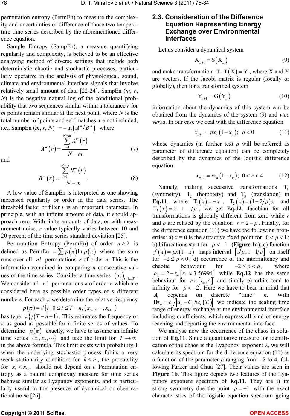

D. T. Mihailović et al. / Natural Science 3 (2011) 75-84 78
permutation entropy (PermEn) to measure the complex-
ity and uncertainties of difference of those two tempera-
ture time series described by the aforementioned differ-
ence equation.
Sample Entropy (SampEn), a measure quantifying
regularity and complexity, is believed to be an effective
analysing method of diverse settings that include both
deterministic chaotic and stochastic processes, particu-
larly operative in the analysis of physiological, sound,
climate and environmental interface signals that involve
relatively small amount of data [22-24]. SampEn (m, r,
N) is the negative natural log of the conditional prob-
ability that two sequences similar within a tolerance r for
m points remain similar at the next point, where N is the
total number of points and self matches are not included,
i.e., SampEn (m, r, N)


ln mm
A
B where
 
1
Nm m
i
mi
A
r
Ar Nm




(7)
and
 
1.
Nm m
i
mi
Br
Br Nm




(8)
A low value of SampEn is interpreted as one showing
increased regularity or order in the data series. The
threshold factor or filter r is an important parameter. In
principle, with an infinite amount of data, it should ap-
proach zero. With finite amounts of data, or with meas-
urement noise, r value typically varies between 10 and
20 percent of the time series standard deviation [25].
Permutation Entropy (PermEn) of order 2n is
defined as PermEn
 
lnpπpπ where the sum
runs over all !n permutations π of order n. This is the
information contained in comparing n consecutive val-
ues of the time series. Consider a time series


1,...
ttT
x.
We consider all !n permutations π of order n which are
considered here as possible order types of n different
numbers. For each π we determine the relative frequency
 

1
#|0, ,,
ttn
pπttTnxx

 
has type
 
1πTn . This estimates the frequency of
π as good as possible for a finite series of values. To
determine

pπ exactly, we have to assume an infinite
time series

12
,,xx and take the limit for T
in the above formula. This limit exists with probability 1
when the underlying stochastic process fulfils a very
weak stationarity condition: for kn, the probability
for ttk
x
x  should not depend on t. Permutation en-
tropy as a natural complexity measure for time series
behaves similar as Lyapunov exponents, and is particu-
larly useful in the presence of dynamical or observa-
tional noise [26].
2.3. Consideration of the Difference
Equation Representing Energy
Exchange over Environmental
Interfaces
Let us consider a dynamical system


1
XSX
nn (9)
and make transformation

T:T XY, where X and Y
are vectors. If the Jacobi matrix is regular (locally or
globally), then for a transformed system

1
YGY
nn (10)
information about the dynamics of this system can be
obtained from the dynamics of the system (9) and vice
versa. In our case we deal with the difference equation

11;0 nnn
xρxxρ


 (11)
whose dynamics (in further text ρ will be referred as
parameter of difference equation) can be completely
described by the dynamics of the logistic difference
equation

11;0 4 nnn
xrxx r


 (12)
Namely, making successive transformations 1
T
(symmetry), 2
T (homotety) and 3 T (translation) in
Eq.11, where


1
T
x
x

,
 
2
T12xρ
x
 and


3
T11xx
ρ
 , we get Eq.12. Jacobian for all
transformations is globally different from zero while r
and ρ are related by the equation 2r
ρ
. Finally, for
the difference equation (11) we have the following prop-
erties: a) x = 0 is the attractive fixed point for 01ρ

;
b) bifurcations start for 1ρ

 (Figure 1a); c) function




1fx ρ
x
x

 maps interval


1,11ρ
ρ
 on itself
for 20ρ

; d) occurrence of the intermittency and
chaotic behaviour for 2ρ
ρ

  where


2 3.56994ρrr

  while Eq.12 has the same
behaviour for


,4rr

 and finally e) orbits tend to
infinity for 2ρ

. Here we have to bear in mind that
1
A
depends on discrete “time” n. With


p
ic Lsi
tcaCbeTD we indicate the scaling time
range of energy exchange at the environmental interface
including coefficients, which express all kind of energy
reaching and departing the environmental interface.
We analyse now the occurrence of the chaos in solu-
tion of Eq.11. Since a quantitative measure for identifi-
cation of the chaos is the Lyapunov exponent λ, we will
calculate its spectrum for the difference equation (11) as
a function of the parameter ρ ranging from –2 to 4, fol-
lowing Parker and Chua [27]. Their values are seen in
Figure 1b. This figure depicts two features of the Lya-
punov exponent spectrum of Eq.11 . They are i) its
strong symmetry due the point 1ρ with the exact
characteristics of the logistic equation spectrum going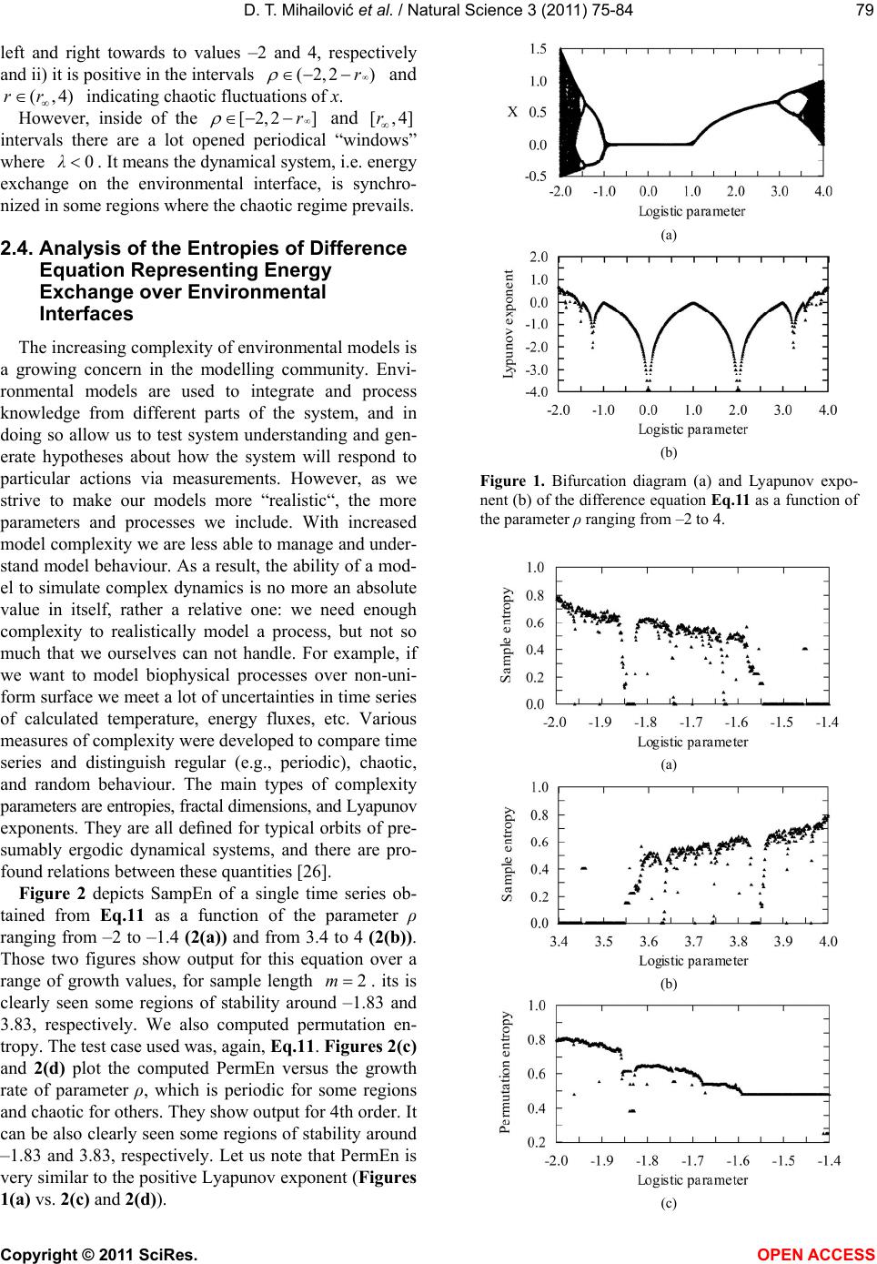

D. T. Mihailović et al. / Natural Science 3 (2011) 75-84
7979
left and right towards to values –2 and 4, respectively
and ii) it is positive in the intervals (2,2)r


  and
(,4)rr

 indicating chaotic fluctuations of x.
However, inside of the [2,2 ]r



 and [,4]r
intervals there are a lot opened periodical “windows”
where 0λ. It means the dynamical system, i.e. energy
exchange on the environmental interface, is synchro-
nized in some regions where the chaotic regime prevails.
2.4. Analysis of the Entropies of Difference
Equation Representing Energy
Exchange over Environmental
Interfaces
The increasing complexity of environmental models is
a growing concern in the modelling community. Envi-
ronmental models are used to integrate and process
knowledge from different parts of the system, and in
doing so allow us to test system understanding and gen-
erate hypotheses about how the system will respond to
particular actions via measurements. However, as we
strive to make our models more “realistic“, the more
parameters and processes we include. With increased
model complexity we are less able to manage and under-
stand model behaviour. As a result, the ability of a mod-
el to simulate complex dynamics is no more an absolute
value in itself, rather a relative one: we need enough
complexity to realistically model a process, but not so
much that we ourselves can not handle. For example, if
we want to model biophysical processes over non-uni-
form surface we meet a lot of uncertainties in time series
of calculated temperature, energy fluxes, etc. Various
measures of complexity were developed to compare time
series and distinguish regular (e.g., periodic), chaotic,
and random behaviour. The main types of complexity
parameters are entropies, fractal dimensions, and Lyapunov
exponents. They are all defined for typical orbits of pre-
sumably ergodic dynamical systems, and there are pro-
found relations between these quantities [26].
Figure 2 depicts SampEn of a single time series ob-
tained from Eq.11 as a function of the parameter ρ
ranging from –2 to –1.4 (2(a )) and from 3.4 to 4 (2(b)).
Those two figures show output for this equation over a
range of growth values, for sample length 2m. its is
clearly seen some regions of stability around –1.83 and
3.83, respectively. We also computed permutation en-
tropy. The test case used was, again, Eq.11. Figures 2(c)
and 2(d) plot the computed PermEn versus the growth
rate of parameter ρ, which is periodic for some regions
and chaotic for others. They show output for 4th order. It
can be also clearly seen some regions of stability around
–1.83 and 3.83, respectively. Let us note that PermEn is
very similar to the positive Lyapunov exponent (Figures
1(a) vs. 2(c) and 2(d)).
(a)
(b)
Figure 1. Bifurcation diagram (a) and Lyapunov expo-
nent (b) of the difference equation Eq.11 as a function of
the parameter ρ ranging from –2 to 4.
(a)
(b)
(c)

D. T. Mihailović et al. / Natural Science 3 (2011) 75-84 80
(d)
Figure 2. Sample entropy as a function of the parameter
ρ ranging from –2 to –1.4 (a) and from 3.4 to 4 (b); per-
mutation entropy as a function of the parameter ρ ranging
from –2 to –1.4 (c) and from 3.4 to 4 (d).
3. ENERGY EXCHANGE BETWEEN
ENVIRONMENTAL INTERFACES
Under the aforementioned conditions, Eqs.11 and 12
represent energy exchange at a uniform environmental
interface. In nature, however, we usually encounter a
mixture of two or more environmental interfaces, for
example, a surface covered by spots consisting of dif-
ferent plant communities and barren soil or any two
other biophysical interfaces. In this case there exist a
number of interacting environmental interfaces. There-
fore, the energy exchange between them is more com-
plex because it has to be described with more equations
having the form of Eqs.11 and 12. Like many other in-
teresting physical problems [28], interaction between
environmental interfaces can be described by the dy-
namics of coupled oscillators. In order to study their
behaviour as a function of coupling strength and nonlin-
earity, we consider the dynamics of two coupled maps
belonging to the same universality class as oscillators.
3.1. Maps Representing Energy Exchange
between Biophysical Environmental
Interfaces
In modelling complex environmental interface sys-
tems, it is also interesting to consider the behaviour of
the following system of two linearly coupled maps





12
11 nnn
xεfrx ε
f
ry
 (13)





21
11 nnn
yεfryεfrx
 (14)
where the map



,1
f
rx rxx
is taken to be the
logistic map with logistic parameters

1
r and

2
r
while, is a coupling parameter. In the case of
 
12
rr

,
two maps are synchronized no matter what the initial
conditions may be, i.e., coupled maps are identical with
a single logistic map. Interesting is the case of
 
12
rr

.
In the following we fix the logistic parameters above and
below the critical value

13.56994r for

1
r and

2
r
respectively. We choose the logistic parameters

1
r
and

2
r and regard the coupling parameter ε as the
controlling parameter. In Figures 3 and 4, the attractors
of the coupled-map are displayed as functions of cou-
pling ε. Figure 3 shows the result of

14r

and

23r

while Figure 4 shows that of

14r

and

22r

. In both cases, for each value of ε we used the
final value of the previous ε and 500 iterations were
plotted. They are two typical examples of the various
values of

1
r and

2
r. One immediately notices sev-
eral interesting features. The fact that there are two cha-
otic regions in both 0ε

and 1ε ends seems odd
at first sight, but after some reflection, one realizes that
very weak ε means very strong

1ε, which brings
chaos first to the variable x and then to y, however weak
the coupling term may be. The most salient feature is the
appearance of a stable period four cycle right after the
period one around 0.77ε

in Figure 3. Another case,
found both in Figure 3 and Figure 4 cases, is the sudden
filling of the x and y space around 0.85ε and above.
The broad window-like region with period four around
0.9ε

in the case of Figure 4 is also noteworthy.
1.0
0.5
0.0
ε
0.00 0.25 0.50 0.75 1.00
0.00 0.25 0.50 0.75 1.00
ε
x
y
1.0
0.5
0.0
Figure 3. Phase diagram for the maps given by Eqs.13
and 14 with (1) 4.0r and (2) 3.0r, and 01


.
For each value of

, the map was iterated 1500 times
from the initial point 0.2, 0.4xy

 to eliminate tran-
sients, and the next 500 iterates were plotted.

D. T. Mihailović et al. / Natural Science 3 (2011) 75-84
8181
1.0
0.5
0.0
ε
0.00 0.25
0.50 0.75 1.00
ε
x y
1.0
0.5
0.00.00 0.25
0.50 0.75 1.00
Figure 4. Phase diagram for the maps given by Eqs.13
and 14 with (1) 4.0r and (2) 2.0r, and 01


.
For each value of

, the map was iterated 1500 times
from the initial point 0.2, 0.4xy to eliminate tran-
sients, and the next 500 iterates were plotted.
3.2. Lyapunov Exponent and Cross Sample
Entropy of Map Representing Energy
Exchange between Biophysical
Environmental Interfaces
Nonlinear dynamical analysis is powerful approach in
understanding biophysical complex systems. We will
consider two parameters included in the archive of this
analysis Lyapunov exponent and cross sample entropy
(Cross-SampEn).
Consider the general vector mapping

1F, 0,1, nn
xxn


  (15)
and its thN iterate





1
FFF
NN
x
x




with

 
1
FF
x
x


. The asymptotic behaviour of a series of
iterates of the map can be characterized by the largest
Lyapunov exponent, which, for an initial point 0
x

is an
attracting region, is defined to be
()
0
ln D( )
lim
N
N
x
λN









(16)
where is the norm of the Jacobi matrix D and

D
N
for the mappings


F
x


and


FN
x
 respectively.
For mapping given by Eqs.13 and 14






 


12
12
112 12
D
121 12
εrxεry
εrx εry


 








(17)
This exponent measures how rapidly two nearby or-
bits in attracting region converge or diverge. It can be
evaluated by noting that






1
000
DDFD
NN
x
xx




;
so if 01 2 ,, ,xxx

 are successive iterates of the map,
then

 


0110
DDDD.
N
N
x
xxx




 (18)
In practice, λ is computed by initially iterating the
map many times to eliminate transient behaviour and
then using a large number N of successive points to
compute the derivative matrix as indicated in Eq.18.
Finally, the quantity ()
0
ln D()
N
x
N


 is used as an
approximate value of the Lyapunov exponent for the
attracting region [29]. This exponent provides a way to
distinguish among periodic, quasiperiodic, and chaotic
motion. Specifically, if 0
x

is part of a stable periodic
orbit of length K, then the norm of the derivative matrix


DK
x

will be less than one for every x in the K
cycle. Thus the exponent will be negative and will char-
acterize the rate at which small perturbations from the
fixed cycle decay. A zero value for the exponent indi-
cates quasiperiodic behaviour in which nearby paths
maintain their distance on average. Finally, when λ be-
comes positive, nearby points in the attracting region
diverge from each other giving chaotic motion. In gen-
eral, the exponent will depend on the initial point used in
the iteration because there may be several stable attrac-
tors, each with a separate basin of attraction [28].
We calculated the Lyapunov exponent λ to see the
behaviour of the coupled maps given by Eqs.13 and 14
depending on different values of coupling parameter ε.
Figures 5(a) an d 5(b) show Lyapunov exponent for the
coupled maps as a function of ε ranging from 0 to 1.
Each point was obtained by iterating 1500 times from
the initial condition to eliminate transient behaviour and
then averaging over another 500 iterations starting from
initial condition (1) 0.20r and (2) 0.25r with 500 ε
values. This simple analysis, where we consider Lyapu-
nov exponent, shows a very interesting features of two
coupled logistic maps representing interaction of two
environmental interfaces, regarded as biophysical com-
plex systems, through exchange of energy between them.
For, example it is seen from Figure 5(a) and 5(b) that
the region with positive Lyapunov exponent, respect to ε,
is more emphasised when the one of the logistic map has
larger values of the logistic parameter.

D. T. Mihailović et al. / Natural Science 3 (2011) 75-84 82
(a)
(b)
(c)
(d)
Figure 5. Lyapunov exponent (a) and (b) and the Cross-Sem-
ple Entropies (c) and (d) of the coupled maps as a function of
coupling parameter ε ranging from 0 to 1 for parameter values
with different the logistic parameters. The logistic equation
with the logistic parameter r = 4.0 is coupled with the logistic
equation having the following logistic parameters: (1) 2r

and (2) 3r

.
Cross-SampEn measure of asynchrony is a recently
introduced technique for comparing two different time
series to assess their degree of asynchrony or dissimilar-
ity [30,31]. Let

 
1, 2,uu uuN





 and

 
1, 2,vvvvN






fix input parameters m and r. Vector sequences:





 
,1, 1xiui uiuim






and





 
,1, 1yjvj vjvjm

 



and N is the number of data points of time series, ,ij

1Nm

. For each iNm

 set




m
i
Brvu=
(number of jNm

such that
 
,
mm
dxi yjr




)


Nm, where j ranges from 1 to Nm. And then
 


1
Nm m
i
mi
Brvu
Brvu Nm




(18)
which is the average value of

m
i
Bvu .
Similarly we define m
A
and m
i
A
as




m
i
A
rvu =
(number of jNm

 such that
 
,
mm
dxi yjr




)


Nm).


 
1
Nm m
i
mi
A
rvu
Arvu Nm




(19)

D. T. Mihailović et al. / Natural Science 3 (2011) 75-84
8383
which is the average value of

m
i
A
vu . And then
 

 
,, ln
m
m
A
rvu
CrossSampEnmrnBrvu






(20)
We applied Cross-SampEn with 5m and 0.05r

for x and y time series. Figures 5(c) and 5(d) show high
synchronisation between them in the interval 0.2-0.8 of
coupling parameter.
4. CONCLUDING REMARKS
We considered a combined approach to the modelling
of environmental interfaces regarded as biophysical
complex systems. They are higher dimensional complex
systems where both of their parts, organization and
temporal dynamics, demand different kinds of formalism.
Therefore, we reported the results of numerical investi-
gation on the systems of two coupled maps, representing
the exchange of energy, of two interacting environ-
mental interfaces. It has been done by calculating the
phase diagrams of the coupled maps for different values
of the logistic and coupling parameters as well as by the
calculation of the Lyapunov exponent and cross sample
entropy. It seems that further analysis of this system will
be useful for understanding the processes of the ex-
change of different quantities between two interacting
environmental interfaces.
5. ACKNOWLEDGEMENTS
The research described here was funded by the Serbian Ministry of
Science and Technology under the project No. III 43007 “Research of
climate changes and their impact on environment. Monitoring of the
impact, adaptation and moderation” for 2011-2014.
REFERENCES
[1] Mihailovic, D.T. and Balaz, I. (2007) An essay about
modeling problems of complex systems in environmental
fluid mechanics. Idojaras, 111, 209-220.
[2] Rosen, R. (1991) Life itself: A comprehensive inquiry
into the nature, origin, and fabrication of life. Columbia
University Press, New York.
[3] Selvam, A.M. and Fadnavis, S. (1998) Signatures of a
universal spectrum for atmospheric interannual variabil-
ity in some disparate climatic regimes. Meteorology and
Atmospheric Physics, 66, 87-112.
doi:10.1007/BF01030450
[4] Sivertsen, T.H. (2005) Discussing the scientific method
and a documentation system of meteorological and bio-
logical parameters. Physics and Chemistry of the Earth,
30, 35-43.
[5] Glazier, J. and Graner, F. (1993) Simulation of the dif-
ferential adhesion driven rearrangement of biological
cells. Physical Review E, 47, 2128-2154.
doi:10.1103/PhysRevE.47.2128
[6] Martins, M.L., Ceotto, G., Alves, G., Bufon, C.C.B.,
Silva, J.M. and Laranjeira, F.F. (2000) Cellular automata
model for citrus variegated chlorosis. Physical Review E,
62, 7024-7030.
doi:10.1103/PhysRevE.62.7024
[7] Nikolov, N., Massman, W. and Schoettle, A. (1995)
Coupling biochemical and biophysical processes at leaf
level: an equilibrium photosynthesis model for leaves of
C3 plants. Ecological Modelling, 80, 205-235.
doi:10.1016/0304-3800(94)00072-P
[8] Niyogi, D.S. and Raman, S. (2001) Numerical modelling
of gas deposition and bidirectional surface–atmosphere
exchanges in mesoscale air pollution systems. In: Boy-
beyi, Z. Ed., Advances in Air Pollution, WIT Publica-
tions, Southampton, 1-51.
[9] Cushman-Roisin, B., Gualtieri, C. and Mihailovic, D.T.
(2008) Environmental fluid mechanics: Current issues
and future outlook. In: Gualtieri, C. and Mihailovic, D.T.
Eds., Fluid Mechanics of Environmental Interfaces,
Taylor & Francis, Leiden, 1-16.
[10] Collier, J.D. (2003) Fundamental properties of self-or-
ganization. In: Arshinov, V. and Fuchs, C. Eds., Causal-
ity, Emergence, Self-Organisation, NIA-Priroda, Mos-
cow, 150-166.
[11] Arshinov, V. and Fuchs, C. (2003) Preface. In: Arshinov,
V. and Fuchs, C. Eds., Causality, Emergence, Self-Or-
ganisation, NIA-Priroda, Moscow, 1-18.
[12] Edmonds, B. (1999) What is Complexity? The philoso-
phy of complexity per se with application to some exam-
ples in evolution. In: Heylighen F., Bollen, J. and Riegler,
A. Eds., The Evolution of Complexity, Kluwer, Dordrecht,
1-17.
[13] Kauffman, S. (1993) The origins of order: Self-organi-
zation and selection in evolution. Oxford University
Press, Oxford.
[14] Heylighen, F. (1999) The growth of structural and func-
tional complexity during evolution. In: Heylighen F.,
Bollen, J. and Riegler, A. Eds., The Evolution of Com-
plexity, Kluwer, Dordrecht, 17-47.
[15] Kaneko, K. (1983) Transition from torus to chaos ac-
companied by the frequency locking with symmetry
breaking - In connection with the coupled logistic map.
Progress of Theoretical Physics, 69, 1427-1442.
doi:10.1143/PTP.69.1427
[16] Midorikawa, S., Takayuki, K. and Taksu, C. (1995)
Folded bifurcation in coupled asymmetric logistic maps.
Progress of Theoretical Physics, 94, 571-575.
doi:10.1143/PTP.94.571
[17] Mihailovic, D.T. (2008) Two interacting environmental
Interfaces: Folded bifurcation in coupled asymmetric lo-
gistic maps. 4th Biennial Meeting: International Con-
gress on Environmental Modelling and Software (iEMSs
2008), 134-140.
[18] Balaz, I. and Mihailovic, D.T. (2008) Evolvable biologi-
cal interfaces: Outline of the new computing system. 4th
Biennial Meeting: International Congress on Environ-
mental Modelling and Software (iEMSs 2008), Barcelona,
7-10 July 2008, 104-113.
[19] Van der Vaart, H.R. (1973) A comparative investigation
of certain difference equations and related differential
equations: implications for model building. Bulletin of
Mathematical Biology, 35, 195-211.

D. T. Mihailović et al. / Natural Science 3 (2011) 75-84 84
[20] Bhumralkar, C.M. (1975) Numerical experiments on the
computation of ground surface temperature in an atmos-
pheric general circulation model. Journal of Applied Me-
teorology, 14, 1246-1258.
doi:10.1175/1520-0450(1975)014%3c1246:NEOTCO%3
e2.0.CO;2
[21] Holtslag A.A. and Van Ulden, A.P. (1983) A simple
scheme for daytime estimates of the surface fluxes from
routine weather data. Journal of Applied Meteorology, 22,
517-529.
doi:10.1175/1520-0450(1983)022%3c0517:ASSFDE%3
e2.0.CO;2
[22] Kennel, M.B., Brown, R. and Abarbanel, H.D.I. (1992)
Determining embedding dimension for phase-space re-
construction using a geometrical construction. Physical
Review A, 45, 3403-3411.
doi:10.1103/PhysRevA.45.3403
[23] Richman, J.S. and Moorman, J.R. (2000) Physiological
time-series analysis using approximate entropy and sam-
ple entropy. American Journal of Physiology: Heart &
Circulatory Physiology, 278, H2039-H2049.
[24] Lake, D.E., Richman, J.S., Griffin, M.P. and Moorman,
J.R. (2002) Sample entropy analysis of neonatal heart
rate variability. American Journal of Physiology: Regu-
latory Integrative and Comparative Physiology, 283,
R789-R797.
[25] Pincus, S.M. (1991) Approximate entropy as a measure
of system complexity. Proceedings of the National
Academy of Sciences of the United States, 88, 2297-2301.
doi:10.1073/pnas.88.6.2297
[26] Bandt, C. and Pompe, B. (2002) Permutation entropy: A
natural complexity measure for time series. Physical Re-
view Letter, 88, 174102.
doi:10.1103/PhysRevLett.88.174102
[27] Parker, T.S. and Chua, L.O. (1989) Practical Numerical
Algorithms for Chaotic Systems. Springer-Verlag, New
York.
[28] Hogg, T. and Huberman, B.A. (1984) Generic behavior
of coupled oscillators. Physical Review A, 29, 275-281.
doi:10.1103/PhysRevA.29.275
[29] Feit, D. (1978) Characteristic exponents and strange
attractors. Communications in Mathematical Physics, 61,
249.
doi:10.1007/BF01940767
[30] Pincus, S. and Singer B.H. (1995) Randomness and de-
grees of irregularity. Proceedings of the National Acad-
emy of Sciences, 93, 2083-2088.
doi:10.1073/pnas.93.5.2083
[31] Pincus, S.M., Mulligan, T., Iranmanesh, A., Gheorghiu,
S., Godschalk, M. and Veldhuis J.D. (1996) Older males
secrete luteinizing hormone and testosterone more ir-
regularly, and jointly more asynchronously, than younger
males. Proceedings of the National Academy of Sciences,
93, 14100-14105.
doi:10.1073/pnas.93.24.14100