Journal of Software Engineering and Applications, 2013, 6, 533-542
http://dx.doi.org/10.4236/jsea.2013.610064 Published Online October 2013 (http://www.scirp.org/journal/jsea)
533
Tuning Recurrent Neural Networks for Recognizing
Handwritten Arabic Words
Esam Qaralleh1, Gheith Abandah2, Fuad Jamour3
1Computer Engineering Department, Princess Sumaya University for Technology, Amman, Jordan; 2Computer Engineering Depart-
ment, The University of Jordan, Amman, Jordan; 3Graduate Student, King Abdullah University of Science and Technology, Thuwal,
Saudi Arabia.
Received August 14th, 2013; revised September 6th, 2013; accepted September 13th, 2013
Copyright © 2013 Esam Qaralleh et al. This is an open access article distributed under the Creative Commons Attribution License,
which permits unrestricted use, distribution, and reproduction in any medium, provided the original work is properly cited.
ABSTRACT
Artificial neural networks have the abilities to learn by example and are capable of solving problems that are hard to
solve using ordinary rule-based programming. They have many design parameters that affect their performance such as
the number and sizes of the hidden layers. Large sizes are slow and small sizes are generally not accurate. Tuning the
neural network size is a hard task because the design space is often large and training is often a long process. We use
design of experiments techniques to tune the recurrent neural network used in an Arabic handwriting recognition system.
We show that best results are achieved with three hidden layers and two subsampling layers. To tune the sizes of these
five layers, we use fractional factorial experiment design to limit the number of experiments to a feasible number.
Moreover, we replicate the experiment configuration multiple times to overcome the randomness in the training proc-
ess. The accuracy and time measurements are analyzed and modeled. The two models are then used to locate network
sizes that are on the Pareto optimal frontier. The approach described in this paper reduces the label error from 26.2% to
19.8%.
Keywords: Optical Character Recognition; Handwritten Arabic Words; Recurrent Neural Networks; Design of
Experiments
1. Introduction
Artificial neural networks are richly connected networks
of simple computational elements. They are capable of
solving problems that linear computing cannot [1]. Re-
current neural networks (RNN) have demonstrated ex-
cellent results in recognizing handwritten Arabic words
[2,3]. Their advantage comes from using the context in-
formation as they contain memory elements and have
cyclical connections.
A neural network has a fixed number of inputs, hidden-
ness, and output nodes arranged in layers. The number
and sizes of these layers determine the performance of
the network, among other network parameters. Small size
networks often suffer limited information processing
power. However, large networks may have redundant
nodes and connections and high computations cost [4,5].
On the other hand, the size of the network determines its
generalization capabilities. Based on what the network
has learned during the training phase, generalization de-
termines its capability to decide upon data unknown to it.
To achieve good generalization, the network size should
be 1) large enough to learn the similarities within same
class samples and at the same time what makes one class
different from other classes and 2) small enough to learn
the differences among the data of the same class [6]. The
latter condition avoids the problem of overfitting or over-
training. Overfitting is the adaptation of the network to
small differences among specific training data set result-
ing in false classification of the test samples [7].
In this paper, we tune a RNN that is used in a system
built for recognizing handwritten Arabic words. We
show how the RNN size is tuned to achieve high recog-
nition accuracy and reasonable training and recognition
times. As the design space of the RNN sizes is huge and
each training experiment takes a long time, we use de-
sign of experiments techniques to collect as much infor-
mation as possible with small number of experiments.
The results of the conducted experiments are analyzed
and modeled. The derived models are used to select a
network size that is on the optimal front and has excel-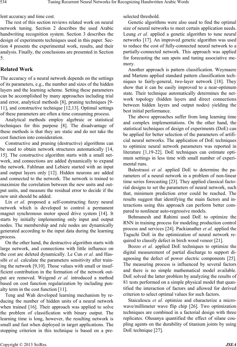

Tuning Recurrent Neural Networks for Recognizing Handwritten Arabic Words
534
lent accuracy and time cost.
The rest of this section reviews related work on neural
network tuning. Section 2 describes the used Arabic
handwriting recognition system. Section 3 describes the
design of experiments techniques used in this paper. Sec-
tion 4 presents the experimental work, results, and their
analysis. Finally, the conclusions are presented in Section
5.
Related Work
The accuracy of a neural network depends on the settings
of its parameters, e.g., the number and sizes of the hidden
layers and the learning scheme. Setting these parameters
can be accomplished by many approaches including trial
and error, analytical methods [8], pruning techniques [9-
11], and constructive technique [12,13]. Optimal settings
of these parameters are often a time consuming process.
Analytical methods employ algebraic or statistical
techniques for this purpose [8]. The disadvantage of
these methods is that they are static and do not take the
cost function into consideration.
Constructive and pruning (destructive) algorithms can
be used to obtain network structures automatically [14,
15]. The constructive algorithm starts with a small net-
work, and connections are added dynamically to expand
the network. Fahlman and Lebiere started with an input
and output layers only [12]. Hidden neurons are added
and connected to the network. The network is trained to
maximize the correlation between the new units and out-
put units, and measure the residual error to decide if the
new unit should be added.
Lin et al. proposed a self-constructing fuzzy neural
network which is developed to control a permanent
magnet synchronous motor speed drive system [14]. It
starts by initially implementing only input and output
nodes. The membership and rule nodes are dynamically
generated according to the input data during the learning
process.
On the other hand, the destructive algorithm starts with
large network, and connections with little influence on
the cost are deleted dynamically. Le Cun et al. and Has-
sibi et al. calculate the parameters sensitivity after train-
ing the network [9,10]. Those values with small or insuf-
ficient contribution in the formation of the network out-
put are removed. Weigend et al. introduced a method
based on cost function regularization by including pen-
alty term in the cost function [11].
Teng and Wah developed learning mechanism by re-
ducing the number of hidden units of a neural network
when trained [16]. Their approach was applied to solve
the problem of classification with binary output. The
learning time is long, however, the resulting network is
small and fast when deployed in target applications. The
stopping criterion in this technique is based on a pre-
selected threshold.
Genetic algorithms were also used to find the optimal
size of neural networks to meet certain application needs.
Leung et al. applied a genetic algorithm to tune neural
networks [17]. An improved genetic algorithm was used
to reduce the cost of fully-connected neural network to a
partially-connected network. This approach was applied
for forecasting the sun spots and tuning associative me-
mory.
Another approach is pattern classification. Weymaere
and Martens applied standard pattern classification tech-
niques to fairly-general, two-layer network [18]. They
show that it can be easily improved to a near-optimum
state. Their technique automatically determines the net-
work topology (hidden layers and direct connections
between hidden layers and output nodes) yielding the
best initial performance.
The above approaches suffer from long learning time
and complex implementations. On the other hand, the
statistical techniques of design of experiments (DoE) can
be applied for better selection of the parameters of artifi-
cial neural networks. The application of DoE techniques
to optimize neural network parameters was reported in
literature [1,19-22]. DoE techniques can estimate opti-
mum settings in less time with small number of experi-
mental runs.
Balestrassi et al. applied DoE to determine the pa-
rameters of a neural network in a problem of non-linear
time series forecasting [23]. They applied classical facto-
rial designs to set the parameters of neural network, such
that, minimum prediction error could be reached. The
results suggest that identifying the main factors and in-
teractions using this approach can perform better com-
pared to nonlinear auto-regressive models.
Behmanesh and Rahimi used DoE to optimize the
RNN in training process for modeling production control
process and services [24]. Packianather et al. applied the
Taguchi DoE in the optimization of neural network re-
quired to classify defect in birch wood veneer [21].
Bozzo et al. applied DoE techniques to optimize the
digital measurement of partial discharge to support di-
agnosing the defect of power electric components [25].
The measuring process is influenced by several factors
and there is no simple mathematical model available.
DoE solved the latter problem by analyzing the results of
81 tests performed on a simple physical model that quan-
tified the interaction of factors and allowed for derived
criterion to select optimal values for such factors.
Staiculescu et al. optimize and characterize a micro-
wave/millimeter wave flip chip [26]. Two optimization
techniques are combined in a factorial design with three
replicates. Olusanya quantified the effect of silane cou-
pling agents on the durability of titanium joints by using
DoE technique [27].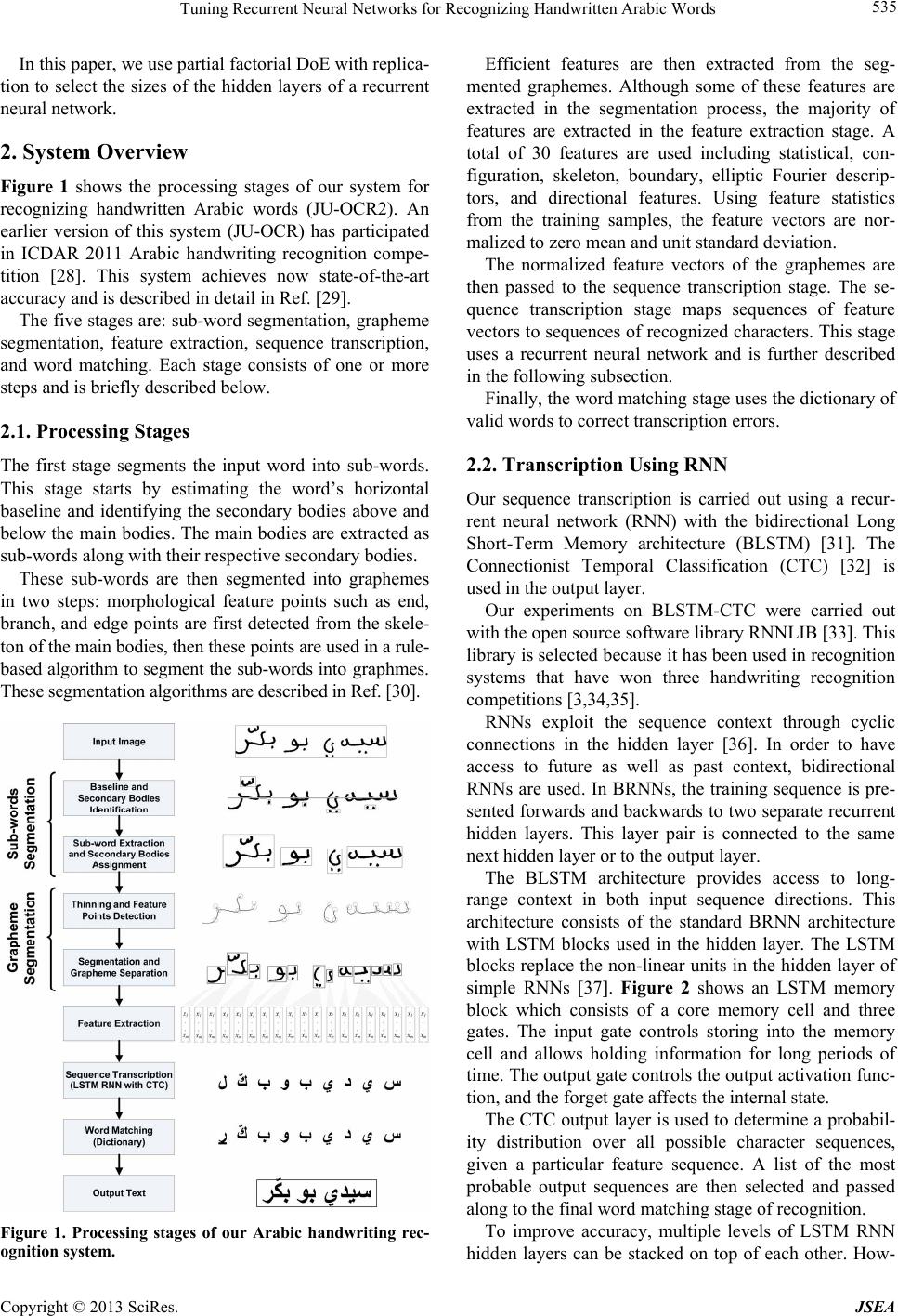

Tuning Recurrent Neural Networks for Recognizing Handwritten Arabic Words 535
In this paper, we use partial factorial DoE with replica-
tion to select the sizes of the hidden layers of a recurrent
neural network.
2. System Overview
Figure 1 shows the processing stages of our system for
recognizing handwritten Arabic words (JU-OCR2). An
earlier version of this system (JU-OCR) has participated
in ICDAR 2011 Arabic handwriting recognition compe-
tition [28]. This system achieves now state-of-the-art
accuracy and is described in detail in Ref. [29].
The five stages are: sub-word segmentation, grapheme
segmentation, feature extraction, sequence transcription,
and word matching. Each stage consists of one or more
steps and is briefly described below.
2.1. Processing Stages
The first stage segments the input word into sub-words.
This stage starts by estimating the word’s horizontal
baseline and identifying the secondary bodies above and
below the main bodies. The main bodies are extracted as
sub-words along with their respective secondary bodies.
These sub-words are then segmented into graphemes
in two steps: morphological feature points such as end,
branch, and edge points are first detected from the skele-
ton of the main bodies, then these points are used in a rule-
based algorithm to segment the sub-words into graphmes.
These segmentation algorithms are described in Ref. [30].
Figure 1. Processing stages of our Arabic handwriting rec-
ognition system.
Efficient features are then extracted from the seg-
mented graphemes. Although some of these features are
extracted in the segmentation process, the majority of
features are extracted in the feature extraction stage. A
total of 30 features are used including statistical, con-
figuration, skeleton, boundary, elliptic Fourier descrip-
tors, and directional features. Using feature statistics
from the training samples, the feature vectors are nor-
malized to zero mean and unit standard deviation.
The normalized feature vectors of the graphemes are
then passed to the sequence transcription stage. The se-
quence transcription stage maps sequences of feature
vectors to sequences of recognized characters. This stage
uses a recurrent neural network and is further described
in the following subsection.
Finally, the word matching stage uses the dictionary of
valid words to correct transcription errors.
2.2. Transcription Using RNN
Our sequence transcription is carried out using a recur-
rent neural network (RNN) with the bidirectional Long
Short-Term Memory architecture (BLSTM) [31]. The
Connectionist Temporal Classification (CTC) [32] is
used in the output layer.
Our experiments on BLSTM-CTC were carried out
with the open source software library RNNLIB [33]. This
library is selected because it has been used in recognition
systems that have won three handwriting recognition
competitions [3,34,35].
RNNs exploit the sequence context through cyclic
connections in the hidden layer [36]. In order to have
access to future as well as past context, bidirectional
RNNs are used. In BRNNs, the training sequence is pre-
sented forwards and backwards to two separate recurrent
hidden layers. This layer pair is connected to the same
next hidden layer or to the output layer.
The BLSTM architecture provides access to long-
range context in both input sequence directions. This
architecture consists of the standard BRNN architecture
with LSTM blocks used in the hidden layer. The LSTM
blocks replace the non-linear units in the hidden layer of
simple RNNs [37]. Figure 2 shows an LSTM memory
block which consists of a core memory cell and three
gates. The input gate controls storing into the memory
cell and allows holding information for long periods of
time. The output gate controls the output activation func-
tion, and the forget gate affects the internal state.
The CTC output layer is used to determine a probabil-
ity distribution over all possible character sequences,
given a particular feature sequence. A list of the most
probable output sequences are then selected and passed
along to the final word matching stage of recognition.
To improve accuracy, multiple levels of LSTM RNN
hidden layers can be stacked on top of each other. How-

Tuning Recurrent Neural Networks for Recognizing Handwritten Arabic Words
536
ever, this leads to a very large number of connections
between the forward and backward layers of successive
levels, and consequently, increase computational cost. As
shown in Figure 3, subsampling layers are used to con-
trol the number of connections between successive levels.
A subsampling layer works as intermediate layer be-
tween two levels, one level feeds forward to the subsam-
pling layer, which in turn feeds forward to the next level.
This way, the number of weights is reduced and is con-
trolled by the size of the subsampling layer.
The performance and computational cost of our RNN
is determined by many factors including its topology
manifested by the number and sizes of the hidden layers
and subsampling layers. In this paper, we use experi-
mental approach to determine the RNN topology.
3. Design of Experiments
In this section, we give an introduction about the design
of experiments techniques and describe some DoE tech-
niques that maximize information with the number of
experiments.
Figure 2. LSTM memory block.
Figure 3. Neural network topology with subsampling layer.
3.1. Introduction to DoE
The goal of DoE is to obtain the maximum information
with the minimum number of experiments [38]. This is
particularly important when each experiment is very long
such as an experiment to train and evaluate a large RNN
using tens of thousands of handwritten samples. DoE is
often needed when the performance of a system is a
function of multiple factors and it is required to select the
optimal levels for these factors or to evaluate the effect
of each factor and the interactions among the factors.
An experimental design consists of specifying the
number of experiments and the factor level combinations
for every experiment. In the simple design, we start with
a base configuration and vary one of the factors at
time to find out how each factor affects performance.
This type of DoE requires 1 experiments,
where i is the number of levels of Factor . However,
this technique is not efficient and cannot evaluate inter-
actions among factors.
k


i

1
k
i
in


1
n
A technique that allows evaluating all effects and
interactions is the full factorial design which includes all
possible combinations of all levels of all factors. This
would sum up to a total of 1 experiments. The
drawback of this technique is getting large number of
experiments when the number of factors and levels is
large.
k
i
in 

An alternative technique is fractional factorial design
which consists of a fraction of the full factorial experi-
ments. Although this technique saves time compared
with the full factorial design, it offers less information
and the evaluation of factor effects and interactions is
less precise. Further detail about factorial DoE is in the
following subsections.
3.2. Factorial Design 2k
One variant of the full factorial design is the fac-
torial design. This design reduces the number of experi-
ments to and allows the evaluation of factor effects
and interactions. This design works well when the system
response is a unidirectional function of each factor.
2k
2k
In this design, only two levels are considered for each
factor. The two levels are usually the minimum level
(referred to by −1) and the maximum level (+1). Table 1
shows this design for two Factors A and B. The table
illustrates for each of the experiments, the levels of
factors A and B and the measured response .
2
2
i
The unit vector (I) in this table is needed for estimate-
ing the average response and the vector (AB) is the
product of A and B and is needed for estimating the in-
teraction between vectors A an B. From the experimental
results, the following model can be derived.
y
0ABAB
yq qAqBqAB

 (1)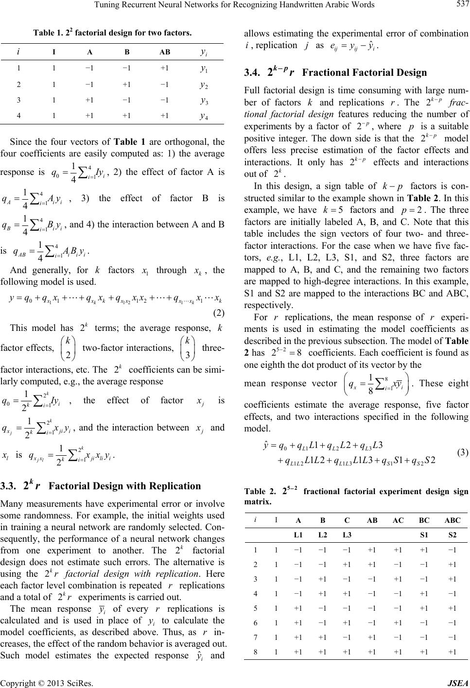

Tuning Recurrent Neural Networks for Recognizing Handwritten Arabic Words 537
Table 1. 22 factorial design for two factors.
i I A B AB i
y
1 1 −1 −1 +1 1
y
2 1 −1 +1 −1 2
y
3 1 +1 −1 −1 3
y
4 1 +1 +1 +1 4
y
Since the four vectors of Table 1 are orthogonal, the
four coefficients are easily computed as: 1) the average
response is 4
01
1
4i
i
q

Iy, 2) the effect of factor A is
4
1
1
4
A
i
q

ii Ay, 3) the effect of factor B is
4
1
1
4
B
ii
i
q

By, and 4) the interaction between A and B
is 4
1
1
4
ABii i
i
qA

By.
And generally, for factors k1
x
through k
x
, the
following model is used.
1121
0112 1
kk
x
xk xxxxk
y
qqxqxqxxq xx 


(2)
This model has terms; the average response,
2kk
factor effects, two-factor interactions, three-
2
k


 3
k



factor interactions, etc. The coefficients can be simi-
larly computed, e.g., the average response
2k
2
01
1
2
k
i
ki
q

Iy, the effect of factor
j
x
is
2
1
1
2
k
j
x
ji i
ki
q

xy, and the interaction between
j
x
and
l
x
is 2
1
1
2
k
jl
x
xj
ki
qx

ilii xy.
3.3. Factorial Design with Replication 2kr
Many measurements have experimental error or involve
some randomness. For example, the initial weights used
in training a neural network are randomly selected. Con-
sequently, the performance of a neural network changes
from one experiment to another. The 2 factorial
design does not estimate such errors. The alternative is
using the factorial design with replication. Here
each factor level combination is repeated replications
and a total of experiments is carried out.
k
2kr
2
r
kr
The mean response i y of every replications is
calculated and is used in place of i to calculate the
model coefficients, as described above. Thus, as in-
creases, the effect of the random behavior is averaged out.
Such model estimates the expected response and
allows estimating the experimental error of combination
, replication as
r
yr
ˆi
y
ijˆ
ijij i
eyy

.
3.4. Fractional Factorial Design 2kp r

Full factorial design is time consuming with large num-
ber of factors and replications . The 2
krkp

frac-
tional factorial design features reducing the number of
experiments by a factor of , where is a suitable
positive integer. The down side is that the
2pp
2kp

model
offers less precise estimation of the factor effects and
interactions. It only has effects and interactions
out of .
2kp
5
2k
In this design, a sign table of factors is con-
structed similar to the example shown in Table 2. In this
example, we have
kp
k

factors and . The three
factors are initially labeled A, B, and C. Note that this
table includes the sign vectors of four two- and three-
factor interactions. For the case when we have five fac-
tors, e.g., L1, L2, L3, S1, and S2, three factors are
mapped to A, B, and C, and the remaining two factors
are mapped to high-degree interactions. In this example,
S1 and S2 are mapped to the interactions BC and ABC,
respectively.
2p
For replications, the mean response of experi-
ments is used in estimating the model coefficients as
described in the previous subsection. The model of Table
2 has
r

r
52
28

coefficients. Each coefficient is found as
one eighth the dot product of its vector by the
mean response vector 8
1
1
8
x
i
i
q





xy


. These eight
coefficients estimate the average response, five factor
effects, and two interactions specified in the following
model.
01
12
q
qL
2 3
131 2
ˆ123
1213 12
LL L
LLLLS S
yqL qLqL
LqLLqSqS
 

(3)
Table 2. 52 2

fractional factorial experiment design sign
matrix.
i I A B C AB AC BCABC
L1L2L3 S1 S2
1 1 −1 −1 −1 +1 +1 +1 −1
2 1 −1 −1 +1 +1 −1 −1 +1
3 1 −1 +1 −1 −1 +1 −1 +1
4 1 −1 +1 +1 −1 −1 +1 −1
5 1 +1 −1 −1 −1 −1 +1 +1
6 1 +1 −1 +1 −1 +1 −1 −1
7 1 +1 +1 −1 +1 −1 −1 −1
8 1 +1 +1 +1 +1 +1 +1 +1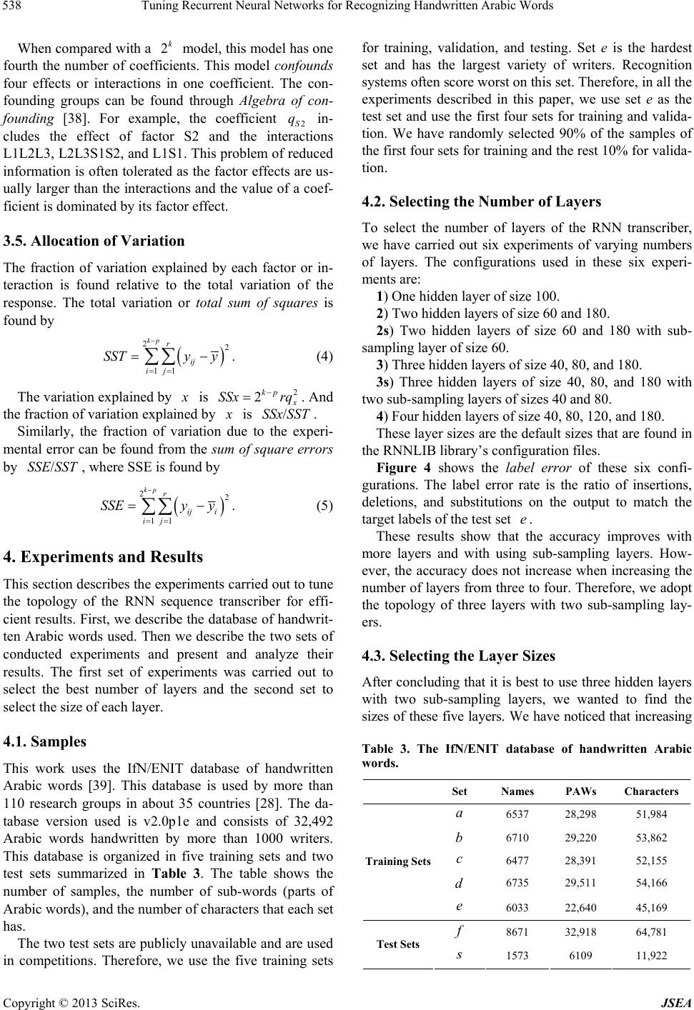

Tuning Recurrent Neural Networks for Recognizing Handwritten Arabic Words
538
When compared with a model, this model has one
fourth the number of coefficients. This model confounds
four effects or interactions in one coefficient. The con-
founding groups can be found through Algebra of con-
founding [38]. For example, the coefficient 2S in-
cludes the effect of factor S2 and the interactions
L1L2L3, L2L3S1S2, and L1S1. This problem of reduced
information is often tolerated as the factor effects are us-
ually larger than the interactions and the value of a coef-
ficient is dominated by its factor effect.
2k
q
3.5. Allocation of Variation
The fraction of variation explained by each factor or in-
teraction is found relative to the total variation of the
response. The total variation or total sum of squares is
found by

22
11
.
kp r
ij
ij
SSTy y



 (4)
The variation explained by
x
is 2 2kp
x
SSx rq

. And
the fraction of variation explained by
x
is . SSTSSx/
Similarly, the fraction of variation due to the experi-
mental error can be found from the sum of square errors
by , where SSE is found by
SSTSSE/

22
11
.
kp r
ij i
ij
SSEy y



 (5)
4. Experiments and Results
This section describes the experiments carried out to tune
the topology of the RNN sequence transcriber for effi-
cient results. First, we describe the database of handwrit-
ten Arabic words used. Then we describe the two sets of
conducted experiments and present and analyze their
results. The first set of experiments was carried out to
select the best number of layers and the second set to
select the size of each layer.
4.1. Samples
This work uses the IfN/ENIT database of handwritten
Arabic words [39]. This database is used by more than
110 research groups in about 35 countries [28]. The da-
tabase version used is v2.0p1e and consists of 32,492
Arabic words handwritten by more than 1000 writers.
This database is organized in five training sets and two
test sets summarized in Table 3. The table shows the
number of samples, the number of sub-words (parts of
Arabic words), and the number of characters that each set
has.
The two test sets are publicly unavailable and are used
in competitions. Therefore, we use the five training sets
for training, validation, and testing. Set e is the hardest
set and has the largest variety of writers. Recognition
systems often score worst on this set. Therefore, in all the
experiments described in this paper, we use set e as the
test set and use the first four sets for training and valida-
tion. We have randomly selected 90% of the samples of
the first four sets for training and the rest 10% for valida-
tion.
4.2. Selecting the Number of Layers
To select the number of layers of the RNN transcriber,
we have carried out six experiments of varying numbers
of layers. The configurations used in these six experi-
ments are:
1) One hidden layer of size 100.
2) Two hidden layers of size 60 and 180.
2s) Two hidden layers of size 60 and 180 with sub-
sampling layer of size 60.
3) Three hidden layers of size 40, 80, and 180.
3s) Three hidden layers of size 40, 80, and 180 with
two sub-sampling layers of sizes 40 and 80.
4) Four hidden layers of size 40, 80, 120, and 180.
These layer sizes are the default sizes that are found in
the RNNLIB library’s configuration files.
Figure 4 shows the label error of these six confi-
gurations. The label error rate is the ratio of insertions,
deletions, and substitutions on the output to match the
target labels of the test set .
e
These results show that the accuracy improves with
more layers and with using sub-sampling layers. How-
ever, the accuracy does not increase when increasing the
number of layers from three to four. Therefore, we adopt
the topology of three layers with two sub-sampling lay-
ers.
4.3. Selecting the Layer Sizes
After concluding that it is best to use three hidden layers
with two sub-sampling layers, we wanted to find the
sizes of these five layers. We have noticed that increasing
Table 3. The IfN/ENIT database of handwritten Arabic
words.
Set Names PAWs Characters
a 6537 28,298 51,984
b 6710 29,220 53,862
c 6477 28,391 52,155
d 6735 29,511 54,166
Training Sets
e 6033 22,640 45,169
f 8671 32,918 64,781
Test Sets
s
1573 6109 11,922

Tuning Recurrent Neural Networks for Recognizing Handwritten Arabic Words 539
Figure 4. The label error for set on neural networks of
six topologies.
e
the layer sizes generally improves the accuracy, but in-
creases the training time and decreases the recognition
speed. Our objective in this set of experiments was to
find layer sizes that give high accuracy and acceptable
training and recognition time.
Selecting the sizes of the five layers is a DoA problem
of five factors. As each factor may take many levels, we
considered design. This consideration is justified be-
cause the RNN response is generally monotonic with the
layer sizes.
2k
However, as the neural network training involves
some randomness, the neural network response varies
from one experiment to another. Therefore, each confi-
guration should be repeated repetitions to get average
values. This is a design. With and
r
2kr5k4r

,
we need 128 experiments that would take too long time.
Therefore, we decided to use design with
, , and . This design reduces the num-
ber of experiments to 32. The selected design is shown in
Table 2 where the three hidden layers are referred to as
L1, L2, and L3, and the two sub-sampling layers are S1
and S2. Table 4 shows the levels used in the eight
configurations. Note that the minimum level (−1) is sel-
ected as one half the default value in the 3S configuration
described in Subsection 4.2 above and the maximum
level (+1) is twice the default value.
2kp r

5k2p4r
Table 5 shows the label error for the eight configure-
tions on four replications. The table also shows the aver-
age label error of each four replications. Note that the
label error decreases from 23.9% for the smallest layer
sizes to 20.1% for the largest sizes. The fraction of varia-
tion due to experimental error (SSE/SST) = 2.0/43.0 =
4.5%.
Table 6 shows the time of each experiment in hours.
Note that this time includes the training and testing times.
These experiments were carried out on Ubuntu 10.10
computers with Intel Core i7-2600 quad processors run-
ning at 3.4 GHz and equipped with 4 GB memory. Note
that this time is highly affected by the neural network
size and ranges from 13.8 hours to 6 days and 19 hours.
Moreover, due to the randomness in training the neural
networks, the training time highly changes from one rep-
lication to another. The fraction of variation due to ex-
perimental error in experiment time (SSE/SST) = 4230/
87,700 = 4.8%.
Table 4. 52 2

fractional factorial experiment design show-
ing layer sizes used.
i L1 L2 L3 S1 S2
1 −1(20) −1(40) −1(90) +1(80) −1(40)
2 −1(20) −1(40) +1(360) −1(20) +1(160)
3 −1(20) +1(160) −1(90) −1(20) +1(160)
4 −1(20) +1(160) +1(360) +1(80) −1(40)
5 +1(80) −1(40) −1(90) +1(80) +1(160)
6 +1(80) −1(40) +1(360) −1(20) −1(40)
7 +1(80) +1(160) −1(90) −1(20) −1(40)
8 +1(80) +1(160) +1(360) +1(80) +1(160)
Table 5. Label error for the eight layer sizes configura-
tions.
i 1
y 2 y 3 y 4 y y
1 23.5% 23.5% 23.6% 23.2% 23.5%
2 21.9% 22.8% 22.0% 22.3% 22.3%
3 23.1% 23.4% 23.5% 23.1% 23.3%
4 21.9% 22.2% 21.8% 22.6% 22.1%
5 21.8% 21.6% 21.5% 21.6% 21.6%
6 22.7% 22.2% 22.0% 21.9% 22.2%
7 23.6% 23.7% 24.3% 24.0% 23.9%
8 20.2% 19.9% 20.3% 19.9% 20.1%
Table 6. Experiment time in hours for the eight layer sizes
configurations.
i 1
t 2 t 3 t 4 t t
1 14.2 14.2 13.5 13.3 13.8
2 159.6 158.0 170.8 165.2 163.4
3 32.8 34.7 34.9 34.2 34.2
4 81.8 72.1 77.4 74.8 76.5
5 17.5 20.9 19.8 29.0 21.8
6 86.1 113.5 50.7 46.9 74.3
7 22.0 16.4 21.4 19.8 19.9
8 101.9 117.0 139.1 139.1 124.2

Tuning Recurrent Neural Networks for Recognizing Handwritten Arabic Words
540
4.4. Analysis
We used the model of Equ. 3 on the results shown in
Tables 5 and 6. Table 7 shows the computed eight
model coefficients for the label error and for the experi-
ment time. This table also shows the fraction of variation
explained by each factor.
The contribution of layer L3 on the label error is the
largest among other factors at 36.5%. The two sub-sam-
pling layers S1 and S2 come next and have almost equal
contributions at 22.0% and 23.1%, respectively.
Layer L3 also has the largest effect on the experiment
time at 69.3%. Next comes the effect of the sub-sampling
layer S2 at 14.4%.
As L3 has the largest contribution, increasing it greatly
lowers the label error, but increases the execution time.
Also, increasing the sizes of S1 and S2 decreases the
label error and increases the execution time. However,
increasing L1 also enhances the label error with little
increase in execution time, similar to S1. On the other
hand, L2 has minor effect, increasing its value does not
give measurable enhancement.
To explore the design space of accuracy and time, we
use Figure 5. This figure shows the results of the eight
configurations of Table 4 (drawn with “+” sign) and the
base, default configuration 3S described in Subsection
1.4.2 (square sign at 45 hrs and 21.0%). Moreover, the
figure shows the estimated label error and experiment
time for 24 additional configurations using the model of
Equation (3) and the coefficients shown in Table 7 (“×”
sign). These 24 configurations are the 32 possible con-
figurations of five binary levels minus the eight configu-
rations of Table 4.
The designer should select configurations that are on
the Pareto op timal frontier. This frontier consists here of
the points of low label error and low experiment time.
The lowest two points are the point of Configuration 8 at
124 hrs and 20.1% and a point from the model at 100 hrs
and 20.0%. This model point has the configuration L1 =
80, L2 = 40, L3 = 360, S1 = 80, and S2 = 160.
This design point was verified experimentally. It
turned out that this configuration achieves 20.2% label
Figure 5. Design space of the label error and experiment
time.
Table 7. Computed model coefficients and fraction of varia-
tion explained by each factor.
0
q1
L
q2
L
q3
L
q 12
L
L
q 13
L
L
q 1S q2S q
22.36−0.413 −0.019 −0.700 0.056 −0.113 −0.544 −0.556
Label
Error


ˆ
y 12.7%0.0%36.5% 0.2% 0.9% 22.0%23.1%
66.0 −5.95 −2.3143.60 14.32 −4.39 −6.92 19.89 Time


ˆ
t 1.3%0.2%69.3% 7.5% 0.7% 1.7%14.4%
error and takes 89 hours. This configuration was adopted
for its excellent accuracy and time trade-off.
A slightly higher accuracy can be achieved using
much larger configuration. We have experimented with a
large configuration of L1 = 100, L2 = 100, L3 = 360, S1
= 120, and S2 = 180. This configuration achieves 19.8%
label error and takes 281 hours.
5. Conclusions
In this paper, we have presented our approach and results
for tuning a recurrent neural network sequence transcri-
ber. This transcriber is used in the recognition stage of
our system for recognizing Arabic handwritten words
(JU-OCR2).
We have used design of experiments techniques to
find a RNN topology that gives good recognition accur-
acy and experiment time. The experimental results pre-
sented in this paper show that it is best to construct the
RNN with three hidden layers and two subsampling
layers.
To select the sizes of these five layers, we designed a
set of experiments using the
r
pk
2
5=
fractional factorial
design. For five factors and , we have
eight experimental configurations. Each configuration is
repeated
k2=p
4=
r
repetitions to overcome the randomness
process in training RNNs.
Our analysis of the label error and experiment time of
the 32 experiments show that the third hidden layer has
the largest contribution on label error and experiment
time, whereas the first hidden layer has the smallest con-
tribution.
Two models were constructed from these experiments
to find the label error and experiment time as functions
of the sizes of the five layers. These models were able to
predict a configuration that lies on the Pareto optimal
frontier. This configuration is L1 = 80, L2 = 40, L3 =
360, S1 = 80, and S2 = 160. We have experimentally
verified that this is an excellent design point that achi-
eves 20.2% label error and takes 89 hours.
6. Acknowledgements
This work was partially supported by the Deanship of the
Scientific Research in the University of Jordan. We

Tuning Recurrent Neural Networks for Recognizing Handwritten Arabic Words 541
would like to thank Alex Graves for making the
RNNLIB publically available [33] and for his help in
using it.
REFERENCES
[1] P. Mehra and B. W. Wah, “Artificial Neural Networks:
Concepts and Theory,” IEEE Computer Society Press,
Los Alamitos, 1992.
[2] A. Graves, “Supervised Sequence Labelling with Recur-
rent Neural Networks,” Studies in Computational Intelli-
gence, Vol. 385, Springer, 2012.
http://dx.doi.org/10.1007/978-3-642-24797-2
[3] V. Märgner and H. El Abed, “ICDAR 2009—Arabic
Handwriting Recognition Competition,” International
Conference on Document Analysis and Recognition, Bar-
celona, 26-29 July 2009, pp. 1383-1387.
[4] X. Yao, “Evolving Artificial Neural Networks,” Pro-
ceedings of the IEEE, Vol. 87, No. 9, 1999, pp. 1423-
1447. http://dx.doi.org/10.1109/5.784219
[5] X. Yao and Y. Liu, “A New Evolutionary System for
Evolving Artificial Neural Networks,” IEEE Transactions
on Neural Networks, Vol. 8, No. 3, 1997, pp. 694-713.
http://dx.doi.org/10.1109/72.572107
[6] S. Theodoridis and K. Koutroumbas, “Pattern Recogni-
tion,” Academic Press, Waltham, 2006.
[7] Y. Chauvin, “Generalization Performance of Overtrained
Back-Propagation Networks,” Neural Networks, Springer,
1990, pp. 45-55.
[8] G. Mirchandani and W. Cao, “On Hidden Nodes for Neu-
ral Nets,” IEEE Transactions on Circuits and Systems,
Vol. 36, No. 5, 1989, pp. 661-664.
http://dx.doi.org/10.1109/31.31313
[9] Y. Le Cun, J. S. Denker, S. A. Solla, R. E. Howard and L.
D. Jackel, “Optimal Brain Damage,” Advances in Neural
Information Processing Systems, Vol. 2, No. 1, 1990, p.
1990.
[10] B. Hassibi, D. G. Stork and G. J. Wolff, “Optimal Brain
Surgeon and General Network Pruning,” International
Conference on Neural Networks, Vol. 1, 1993, pp. 293-
299. http://dx.doi.org/10.1109/ICNN.1993.298572
[11] A. S. Weigend, D. E. Rumelhart and B. A. Huberman,
“Back-Propagation, Weight-Elimination and Time Series
Prediction,” Proceedings of 1990 Connectionist Models
Summer School, Vol. 105, Morgan Kaufmann, 1990.
[12] S. E. Fahlman and C. Lebiere, “The Cascadecorrelation
Learning Architecture,” Technical Report, Computer Sci-
ence Department, Carnegie Mellon University, 1989.
[13] S. J. Perantonis, N. Ampazis and V. Virvilis, “A Learning
Framework for Neural Networks Using Constrained Op-
timization Methods,” Annals of Operations Res ea rc h, Vol.
99, No. 1-4, 2000, pp. 385-401.
http://dx.doi.org/10.1023/A:1019240304484
[14] F.-J. Lin, C.-H. Lin and P.-H. Shen, “Selfconstructing
Fuzzy Neural Network Speed Controller for Permanent-
Magnet Synchronous Motor Drive,” IEEE Transactions
on Fuzzy Systems, Vol. 9, No. 5, 2001, pp. 751-759.
http://dx.doi.org/10.1109/91.963761
[15] M. C. Mozer and P. Smolensky, “Using Relevance to Re-
duce Network Size Automatically,” Connection Science,
Vol. 1, No. 1, 1989, pp. 3-16.
http://dx.doi.org/10.1080/09540098908915626
[16] C.-C. Teng and B. W. Wah, “Automated Learning for Re-
ducing the Configuration of a Feedforward Neural Net-
work,” IEEE Transactions on Neural Networks, Vol. 7,
No. 5, 1996, pp. 1072-1085.
http://dx.doi.org/10.1109/72.536305
[17] F. H.-F. Leung, H.-K. Lam, S.-H. Ling and P. K.-S. Tam,
“Tuning of the Structure and Parameters of a Neural Net-
work Using an Improved Genetic Algorithm,” IEEE
Transactions on Neural Networks, Vol. 14, No. 1, 2003,
pp. 79-88. http://dx.doi.org/10.1109/TNN.2002.804317
[18] N. Weymaere and J.-P. Martens, “On the Initialization
and Optimization of Multilayer Perceptrons,” IEEE Tran-
sactions on Neural Networks, Vol. 5, No. 5, 1994, pp.
738-751. http://dx.doi.org/10.1109/72.317726
[19] W. Sukthomya and J. Tannock, “The Optimisation of
Neural Network Parameters Using Taguchi’s Design of
Experiments Approach: An Application in Manufacturing
Process Modelling,” Neural Computing & Applications,
Vol. 14, No. 4, 2005, pp. 337-344.
http://dx.doi.org/10.1007/s00521-005-0470-3
[20] Y.-S. Kim and B.-J. Yum, “Robust Design of Multilayer
Feedforward Neural Networks: An Experimental Ap-
proach,” Engineering Applications of Artificial Intelli-
gence, Vol. 17, No. 3, 2004, pp. 249-263.
http://dx.doi.org/10.1016/j.engappai.2003.12.005
[21] M. Packianather, P. Drake and H. Rowlands, “Optimizing
the Parameters of Multilayered Feedforward Neural Net-
works through Taguchi Design of Experiments,” Quality
and Reliability Engineering International, Vol. 16, No. 6,
2000, pp. 461-473.
http://dx.doi.org/10.1002/1099-1638(200011/12)16:6<46
1::AID-QRE341>3.0.CO;2-G
[22] S. Yang and G. Lee, “Neural Network Design by Using
Taguchi Method,” Journal of Dynamic Systems, Meas-
urement, and Control, Vol. 121, No. 3, 1999, pp. 560-563.
http://dx.doi.org/10.1115/1.2802515
[23] P. Balestrassi, E. Popova, A. d. Paiva and J. Marangon
Lima, “Design of Experiments on Neural Network’s
Training for Nonlinear Time Series Forecasting,” Neuro-
computing, Vol. 72, No. 4, 2009, pp. 1160-1178.
http://dx.doi.org/10.1016/j.neucom.2008.02.002
[24] R. Behmanesh and I. Rahimi, “Control Chart Forecasting:
A Hybrid Model Using Recurrent Neural Network, De-
sign of Experiments and Regression,” Proceedings of
Business Engineering and Industrial Applications Collo-
quium, Kuala Lumpur, 7-8 April 2012, pp. 435-439.
[25] R. Bozzo, G. Coletti, C. Gemme and F. Guastavino, “Ap-
plication of Design of Experiment Techniques to Meas-
urement Procedures: An Example of Optimization Appli-
ed to the Digital Measurement of Partial Discharges,”
Proceedings of Sensing, Processing, Networking, Instru-
men ta tio n and Measurement Technology Confe re nce , Vol.
1, 1997, pp. 470-475.
[26] D. Staiculescu, J. Laskar and M. M. Tentzeris, “Design of

Tuning Recurrent Neural Networks for Recognizing Handwritten Arabic Words
542
Experiments (DOE) Technique for Microwave/Millimeter
Wave Flip-Chip Optimization,” International Journal of
Numerical Modelling: Electronic Networks, Devices and
Fields, Vol. 16, No. 2, 2003, pp. 97-103.
http://dx.doi.org/10.1002/jnm.485
[27] A. Olusanya, “The Use of Design of Experiments Tech-
niques to Determine the Relative Effectiveness of Silane
Coupling Agents on the Durability of Titanium Alloy
Joints: A Case Study,” Techical Report CMMT (A) 128,
National Physical Laboratory, 1998.
[28] V. Märgner and H. El Abed, “ICDAR 2011—Arabic
Handwriting Recognition Competition,” International
Conference on Document Analysis and Recognition, Bei-
jing, 18-21 September 2011, pp. 1444-1448.
[29] G. Abandah, F. Jamour and E. Qaralleh, “Recognizing
Handwritten Arabic Words Using Grapheme Segmenta-
tion and Recurrent Neural Networks,” Submitted.
[30] G. Abandah and F. Jamour, “Recognizing Handwritten
Arabic Script through Efficient Skeleton-Based Graph-
eme Segmentation Algorithm,” 10th International Con-
ference on Intelligent Systems Design and Applications,
Cairo, 29 November-1 December 2010, pp. 977-982.
[31] A. Graves and J. Schmidhuber, “Framewise Phoneme
Classification with Bidirectional LSTM and Other Neural
Network Architectures,” Neural Networks, Vol. 18, No.
5-6, 2005, pp. 602-610.
http://dx.doi.org/10.1016/j.neunet.2005.06.042
[32] A. Graves, S. Fernández, F. Gomez and J. Schmidhuber,
“Connectionist Temporal Classification: Labelling Un-
segmented Sequence Data with Recurrent Neural Net-
works,” Proceedings of International Conference on Ma-
chine Learning, Pittsburgh, 25-26 June 2006.
[33] A. Graves, “RNNLIB: A Recurrent Neural Network Li-
brary for Sequence Learning Problems,” 2013.
http://sourceforge.net/projects/rnnl/
[34] E. Grosicki and H. El Abed, “ICDAR 2009 Handwriting
Recognition Competition,” International Conference on
Document Analysis and Recognition, Barcelona, 26-29
July 2009, pp. 1398-1402.
[35] S. Mozaffari and H. Soltanizadeh, “ICDAR 2009 Hand-
Written Farsi/Arabic Character Recognition Competi-
tion,” International Conference on Document Analysis
and Recognition, Barcelona, 26-29 July 2009, pp. 1413-
1417.
[36] A. Graves, “Supervised Sequence Labelling with Recur-
rent Neural Networks,” PhD Thesis, Technische Univer-
sität München, 2008.
[37] S. Hochreiter and J. Schmidhuber, “Long Short-Term
Memory,” Neural Computation, Vol. 9, No. 8, 1997, pp.
1735-1780. http://dx.doi.org/10.1162/neco.1997.9.8.1735
[38] R. Jain, “The Art of Computer Systems Performance
Analysis: Techniques for Experimental Design, Meas-
urement, Simulation and Modeling,” John Wiley & Sons,
New York, 1991.
[39] M. Pechwitz, S. S. Maddouri, V. Märgner, N. Ellouze and
H. Amiri, “IFN/ENIT—Database of Handwritten Arabic
Words,” 7th Colloque International Francophone sur
l’Ecrit et le Docume nt , 2002, pp. 129-136.
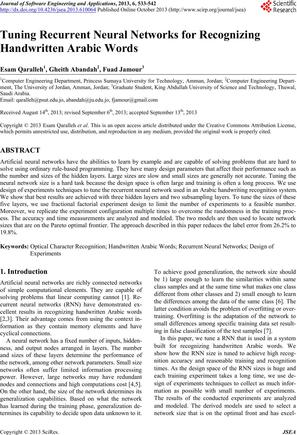