 Open Journal of Applied Sciences, 2013, 3, 337-344 http://dx.doi.org/10.4236/ojapps.2013.35044 Published Online September 2013 (http://www.scirp.org/journal/ojapps) Evaluation of Reliability and Availability Characteristics of a Repairable System with Active Parallel Units Ibrahim Yusuf1*, Fatima Salman Koki2 1Department of Mathematical Sciences, Bayero University, Kano, Nigeria 2Department of Physics, Bayero University, Kano Email: *Ibrahimyusuffagge@gmail.com, FatimaSK2775@gmail.com Received June 5, 2013; revised July 15, 2012; accepted July 22, 2013 Copyright © 2013 Ibrahim Yusuf, Fatima Salman Koki. This is an open access article distributed under the Creative Commons At- tribution License, which permits unrestricted use, distribution, and reproduction in any medium, provided the original work is prop- erly cited. ABSTRACT In this paper, we study the reliability and availability characteristics of a repairable system consisting of two subsystems A and B in series. Subsystem A consists of two units A1 and A2 operating in active parallel while subsystem B is a sin- gle unit. Failure and repair times are assumed exponential. The explicit expressions of reliability and availability char- acteristics like mean time to system failure (MTSF), system availability, busy period and profit function are derived using Kolmogorov forward equations method. Various cases are analyzed graphically to investigate the impacts of sys- tem parameters on MTSF, availability, busy period and profit function. Keywords: Active Parallel; Reliability; Availability; Mean Time to System Failure 1. Introduction Reliability is vital for prop er utilization and maintenance of any system. It involves techniques for increasing sys- tem effectiveness through reducing failure frequency and maintenance-cost minimization. Adequate maintenance management is vital in reducing the adverse effect of equipment failures and maintenance cost and in maxi- mizing equipmen t av ailability . Th e in crease in equipment availability means less maintenance cost, higher produc- tivity and higher profit. There are systems of three units in which two/three units are sufficient to perform the entire function of the system. Such systems are called 2- out-of-3 or 3-out-of-3 redundant systems. These sys- tems have wide application in the real world. The com- munication system with three transmitters can be sited as a good example of 2-out-of-3 redundant system. One of the commonly used forms of redundancy is active paral- lel system, which often finds applications in various in- dustrial or other types of setup. Due to their importance in industries and system design, models of redundant sys- tems as well as methods of evaluating system reliability and availability hav e been research ed in order to improv e the system effectiveness (see, for instance, [1] and [2]). S. V. Amari et al. [3] show that the reliability of systems subject to imperfect fault-coverage decreases after a cer- tain level of active redundancy. K.-H. Wang and B. D. Sivazlian [4] deal with the reliability characteristics of a multiple-server unit system with warm standby units with exponential failure and exponential repair time distribu- tions. Steady-state availability and the mean time to sys- tem failure of a repairable system with warm standbys plus balking and reneging were studied by J.-C. Ke and K.-H. Wang [5,6]. K.-H. Wang et al. [7] deals with the reliability and sensitivity analysis of a system with M operating machines, S warm standbys, and a repairable service station. The problem considered in this paper is different from the work of K. M. El-Said et al. [1,2]. Th e main contribution of this paper is two-fold. The first is to develop the explicit expressions for MTSF, system avail- ability, busy period and profit function. The second is to perform a parametric investigation of various system parameters on MTSF, system availability and profit func- tion and capture their effects on MTSF, availability, busy period and profit function. The rest of the paper is organ- ized as follows. Section 2 gives the notations, assump- tions of the study, the reliability block diagram and the states of the system. Section 3 gives the states of the sys- tem. Section 4 deals with models formulation. The results of our numerical simulations are presented and discussed in Section 5. Section 6 i s the conclusion of the paper. *Corresponding a uthor. C opyright © 2013 SciRes. OJAppS  I. YUSUF, F. S. KOKI 338 2. Notations and Assumptions 2.1. Notations ai: Type i repair rate of unit Ai in operation, i = 1, 2. βi: Type i failure rate of unit in operation Ai, i = 1, 2. η: Type III repair rate of subsystem B in operation. δ: Type III failure rate of subsystem B in operation. 2.2. Assumptions 1) The systems consist of two dissimilar subsystems A and B in series; 2) Subsystem A consist of two units A1 and A2 in active parallel; 3) The system work in a re-duced capacity at the failure of un it A1 or A2; 4) Sub- sys-tem B is a single unit; 5) The systems have two states: normal and failure. 6) Unit failure and repair rates are constant; 7) Repair is as good as new; 8) Failure and re-pair time are assumed exponential; 9) The system fail at the failure of A1 and A2 or subsystem B; 10) The sys- tem is under the attention of one repairman. 3. States of the System 1) State S0: Units A1, A2 and subsystem B are working, the system is working. 2) State S1: Unit A1 is under Type I repair, unit A2 is working, subsystem B is working, and the system is working. 3) State S2: Unit A1 is working, unit A2 is under Type II repair, subsystem B is working, and the system is working. 4) State S3: Unit A1 and A2 are good, subsystem B is under Type III repair, and the system failed. 5) State S4: Unit A1 is under Type I repair, unit A2 is good, subsystem B is under Type III repair, and the system failed. 6) State S5: Unit A1 is under Type I repair, unit A2 is under Type I repair, subsystem B is good, and the system failed. 7) State S6: Unit A1 is under Type I repair, unit A2 is under Type II, subsystem B is good, and the system failed. 8) State S7: Unit A1 is good, unit A2 is under Type II repair, subsystem B is under Type III repair, and the system failed. 9) State S8: Unit A1 is under Type II repair, unit A2 is under Type II, sub- system B is good, and the system failed. 4. Models Formulation 4.1. Mean Time to System Failure for System Let be the probability row vector at time t, then the initial conditions for this problem are as follows: Pt 01234 5678 0,0, 0,0, 0, 00, 0,0, 0 1,0,0,0,0,0,0,0,0 PPPPP PPPPP we obtain the following system of differential equations from Figure 1 above: 0 S 1 S 2 S 4 S 7 S 3 S 8 S 6 S 5 S 1 1 1 1 1 2 2 2 2 2 1 1 2 2 Figure 1. Schematic diagram of the System. 012 011 22 3 1112110 41526 2212 220 167 28 3301427 414 1 515 11 6 d d d d d d d d d d d d d d Pt Pt αPt t Pt Pt Pt Pt Pt t Pt PtPt Pt Pt Pt t Pt PtPt Pt Pt δPt PtPt t Pt Pt Pt t Pt Pt Pt t Pt t 12621 12 727 2 828 22 d d d d PtPt Pt Pt Pt Pt t Pt Pt Pt t (1) The above system of differential equations can be written in matrix form as PAP (2) where 112 121 2 23 1 12 4 11 21 5 6 22 00000 000 0 0000 000 00 000 0000 0000 000 00000 0000 000 0000 000 h hη h Aδh h h 2 0 Copyright © 2013 SciRes. OJAppS  I. YUSUF, F. S. KOKI Copyright © 2013 SciRes. OJAppS 339 4.2. Availability Analysis where 112 2112 3212 41 512 62 h h h h h h For the availability case of Figure 2 following [1,10] using the initial condition in subsection 4.1 for this sys- tem. 01234 5678 0,0, 0,0, 0, (0) 0, 0,0, 0 1,0,0,0,0,0,0,0,0 PPPPP PPPPP The system of differential equations in (1) for the sys- tem above can be expressed in matrix form as: It is difficult to evaluate the transient solutions, hence we follow [8,9], the procedure to develop the explicit expression for MTSF is to delete the fourth row to ninth, fourth to ninth column of matrix A and take the transpose to produce a new matrix, say Q. The expected time to reach an absorbing state is obtained from Let T be the time to failure of the system. The steady-state availability is given by 012T APPP (4) In steady state, the derivatives of state probabilities become zero, 11 0 absorbing1 1 01MTSF 1 PP N ETP QD (3) AP 0 (5) where 12 12 1112 22 () ()0 0( Q 12 ) 1112 212 1212 2112 Nαββδα ββδ βα ββδ βαββδ 3 0 112 1 121 2 2231 2 312 4 4 5 11 621 5 76 8 22 00000 0 00000 0000 0 0000 00 0000000 0 00000000 000000 0 00 000000 00 000000 P hαα η Pβhηα α Pβhαηα P δηαα P δh Pβα Pββh P δh P βα 33 1122111221 2 2222 2 21121121 22222 12 2212112 212 1212 2 3333 33 62 Dααδα βδαβδα βδββδ αβ βββδββ βδ αββδβδ αδ αδ αβ αββββδ αβδ using the normalizing condition 01238 1PPPP P (6) We substitute (6) in the last of row of (5). The result- ing matrix is 0 1112 121 2 2 231 2 312 4 4 11 521 5 6 6 22 7 8 00000 000 0 0000 000 00 000 0000 0000 000 000000 0000 000 0000 000 P Ph h P h P h P Ph h P P P 0 1 2 3 4 5 6 7 8 P P P P P P P P P  I. YUSUF, F. S. KOKI 340 0 112 1 121 2 2 23 12 3 12 4 4 5 11 6 21 5 7 6 8 () 00 000 () 00 00 () 0000 () 000 00 () 0000 000 () 0 000000 () 000000 () 0000 000 () 11111 1111 P h P h P h P P h P P h P h P 0 0 0 0 0 0 0 0 1 Thus, the expression for AT is 2 2 T N AD where 222 22 1221 21212 1122111 22 22 212 22222 2122111221211121221212 22222 12121 2 121 22 22 2 N 22 2 12 12 111 2 22 2 2222112 112122 12121 22222 2 12211 12112112 2 122 22 22221121212122121 2 2 2 42232343323223422 33224234323233 2121212121212 1212121212 233323233323222222 22222 1 2212112212121 2121 21 21 21 23 12 2 22 42 3 D 2232322 42322333342 112 121121211212212 32223 2322243342424233 122121212 121121122122122 332322 12112212 334 2 23322 22 43 2222323443 112112112121 212 32323222222 23323224 12121212 12121212 121121121121 33223223223 122122 112122 22 2 242 222 22 33 32323 121 12112121212 2323 23 223223322322232 12121212121212121222 21 2121 4232232223223232 122 112122122 12212 2 22 3 32 2322322 122121 2 2222222 2222222 22222 1221221221212 1212 12121212 222 332 422332332 422 24233 1212121212212112 121 32 2242222 22 232 121 2433 223 223223332323 121122122122 12112112121212 2323 23 223223322322 12121212121212121222 21 2 232 4 1211 2222 22 3 2322 322232232322322 221121 221 221 22121 22 3222222222 222 2222222 1211 221 221 221 2121212121 2 2222223 12121212 12 32 3 22 24222 2 32422332332 422 242223 1212 212112 112 2 4.3. Busy Period Analysis Using the initial condition in subsection 4.1 above as for reliability case and (5) and (6), the steady-state busy period is 3 02 1N BP D (7) Copyright © 2013 SciRes. OJAppS  I. YUSUF, F. S. KOKI Copyright © 2013 SciRes. OJAppS 341 from Figure 11 the busy period increases as increase. Similar results can be observed in Figures 4, 7, 13 and 15 with respect to where 4.4. Profit Analysis 1 . In these figures, MTSF, availability and profit de- crease as 1 increases while busy period increase with The system/units are subjected to corrective maintenance at fa ilu re as can be observed in states 1-8. From Figure 1, the repairman is busy performing corrective maintenance action to the units/system at failure in states 1-8. Ac- cording to [8,9], the expected profit per unit time in- curred to the system in the steady-state is given by: Profit = total revenue generated – cost in curred for repairing the failed units. A 1 A 2 B Figure 2. Reliability block diagram of the system. 01 PFCACB (8) where PF2: is the profit incurred to the system, C0: is the revenue per unit up time of the system, C1: is the cost per unit time which the system is under repair. 5. Results and Discussions In this section, we numerically obtained the results for mean time to system failure, system availability, busy period and profit function for all the developed models. For the model analysis, the following set of parameters values are fixed throughout the simulations for consis- tency: 1 = 0.05, 2 = 0.2, 1 = 0.5, 2 = 0.01, = 0.1, = 0.5 in Figures 3-7 and assumed 2 = 0.7, in Figures 8-17, C0 = 900,000, C1 = 100,000 in Fig- ures 14-17. Effect of on MTSF, steady-state availability, busy period and profit can be observed in Figures 5, 6, 11 and 16. From Figures 5, 6 and 16, it is evident that the MTSF, availability and profit decrease as increases while Figure 3. Effect of 1 on MTSF. 42232343 323223422 33224234323 3121212121212 12121212 233 233 323 2333232222 222 12 12212112212121212 1212 222223 121 12 2 22 4 23 N 2232322 423223333 112 1211212112122 4232223232 224334242 12122121212121 121122 423333232 2 1 221 221211 221 33 4 22332 222 422232 222 211 21121121 32344332323222232 12121 2121 21212121 212121 21 22 2222222224323 1221211212 1221221 422 22 22 53 2222 211 22 2223 232223324 1 2112212121212121121121 32323232332232 2 1211 212121212212121 2 21 21 23 2 122 2 224 5 2322 2 23 242322333323224 121122 122122121 121121 33223 22322322333232323 122122112122121121121212121 2323 1212121 21 22 222 2 2 23 2223322322 232 2121221 222212121 42 3223 22232 232 322322322 122 112122122 12212122121 2222222 2222 122 1221221212 23 32 32 2242 22222222 121212121 212 222332 422332332 422 242 1212121 21221211 2 222 2 2  I. YUSUF, F. S. KOKI 342 β 1 Figure 4. Effect of 1 on MTSF Figure 5. Effect of on MTSF. Figure 6. Effect of on availability. Figure 7. effect of 1 on availability. η Figure 8. Effect of on availability. Figure 9. Effect of 1 on availability. increase in 1 as can be seen in Figure 13. Results of MTSF, steady-state availability, busy period and profit Copyright © 2013 SciRes. OJAppS 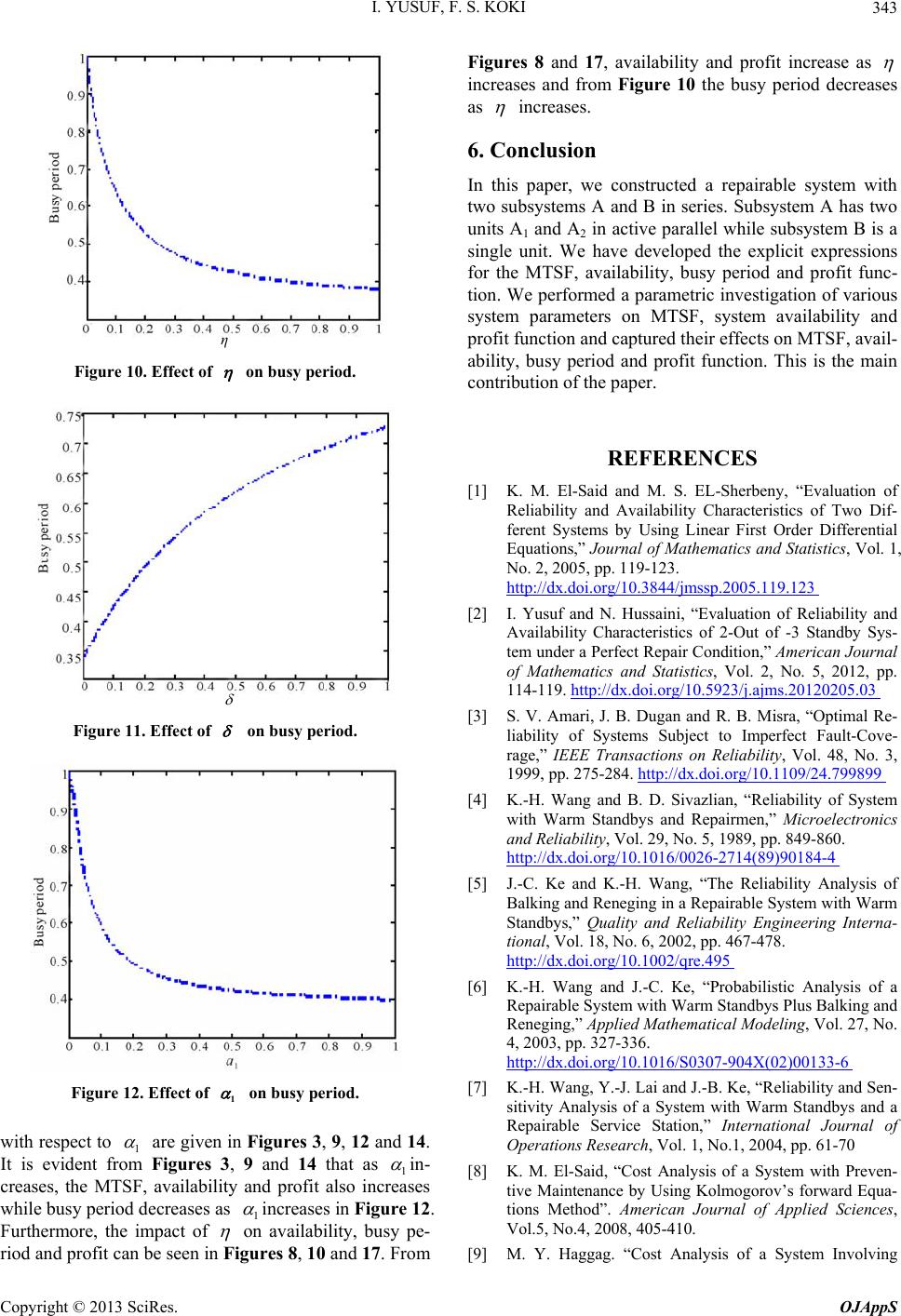 I. YUSUF, F. S. KOKI 343 η Figure 10. Effect of on busy period. Figure 11. Effect of on busy period. Figure 12. Effect of 1 on busy period. with respect to 1 are given in Figures 3, 9, 12 and 14. It is evident from Figures 3, 9 and 14 that as 1 in- creases, the MTSF, availability and profit also increases while busy period decreases as 1 increases in Figure 12. Furthermore, the impact of on availability, busy pe- riod and profit can be seen in Figures 8, 10 and 17. From Figures 8 and 17, availability and profit increase as increases and from Figure 10 the busy period decreases as increases. 6. Conclusion In this paper, we constructed a repairable system with two subsystems A and B in series. Subsystem A has two units A1 and A2 in active parallel while subsystem B is a single unit. We have developed the explicit expressions for the MTSF, availability, busy period and profit func- tion. We performed a parametric investigation of various system parameters on MTSF, system availability and profit function and captured their effects on MTSF, avail- ability, busy period and profit function. This is the main contribution of the paper. REFERENCES [1] K. M. El-Said and M. S. EL-Sherbeny, “Evaluation of Reliability and Availability Characteristics of Two Dif- ferent Systems by Using Linear First Order Differential Equations,” Journal of Mathematics and Statistics, Vol. 1, No. 2, 2005, pp. 119-123. http://dx.doi.org/10.3844/jmssp.2005.119.123 [2] I. Yusuf and N. Hussaini, “Evaluation of Reliability and Availability Characteristics of 2-Out of -3 Standby Sys- tem under a Perfect Repair Condition,” American Journal of Mathematics and Statistics, Vol. 2, No. 5, 2012, pp. 114-119. http://dx.doi.org/10.5923/j.ajms.20120205.03 [3] S. V. Amari, J. B. Dugan and R. B. Misra, “Optimal Re- liability of Systems Subject to Imperfect Fault-Cove- rage,” IEEE Transactions on Reliability, Vol. 48, No. 3, 1999, pp. 275-284. http://dx.doi.org/10.1109/24.799899 [4] K.-H. Wang and B. D. Sivazlian, “Reliability of System with Warm Standbys and Repairmen,” Microelectronics and Reliability, Vol. 29, No. 5, 1989, pp. 849-860. http://dx.doi.org/10.1016/0026-2714(89)90184-4 [5] J.-C. Ke and K.-H. Wang, “The Reliability Analysis of Balking and Reneging in a Repairable System with Warm Standbys,” Quality and Reliability Engineering Interna- tional, Vol. 18, No. 6, 2002, pp. 467-478. http://dx.doi.org/10.1002/qre.495 [6] K.-H. Wang and J.-C. Ke, “Probabilistic Analysis of a Repairable System with Warm Standbys Plus Balking and Reneging,” Applied Mathematical Modeling, Vol. 27, No. 4, 2003, pp. 327-336. http://dx.doi.org/10.1016/S0307-904X(02)00133-6 [7] K.-H. Wang, Y.-J. Lai and J.-B. Ke, “Reliability and Sen- sitivity Analysis of a System with Warm Standbys and a Repairable Service Station,” International Journal of Operations Research, Vol. 1, No.1, 2004, pp. 61-70 [8] K. M. El-Said, “Cost Analysis of a System with Preven- tive Maintenance by Using Kolmogorov’s forward Equa- tions Method”. American Journal of Applied Sciences, Vol.5, No.4, 2008, 405-410. [9] M. Y. Haggag. “Cost Analysis of a System Involving Copyright © 2013 SciRes. OJAppS  I. YUSUF, F. S. KOKI Copyright © 2013 SciRes. OJAppS 344 Common Cause Failures and Preventive Maintenance”. Journal of Mathematics and Statistics, Vol. 5, No.4, 2009. pp 305-310. http://dx.doi.org/10.3844/jmssp.2009.305.310 [10] M. Y. Haggag, “Cost Analysis of k-Out-of-n Repairable System with Dependent Failure and Standby Support Us- ing Kolmogorov’s Forward Equations Method,” Journal of Mathematics and Statistics, Vol. 5, No. 4, 2009. pp. 401-407.
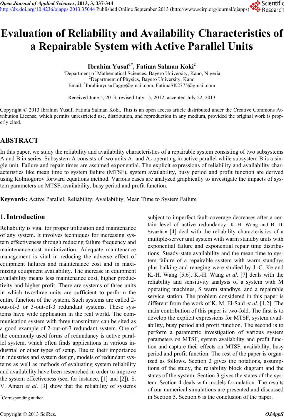
|