 Journal of Applied Mathematics and Physics, 2013, 1, 55-59 http://dx.doi.org/10.4236/jamp.2013.13009 Published Online August 2013 (http://www.scirp.org/journal/jamp) Some Results on the Differential Geometry of Spacelike Curves in De-Sitter Space Tunahan Turhan1*, Nihat Ayyildiz2 1Seydişehir Vocational School, Necmettin Erbakan University, Konya, Turkey 2Department of Mathematics, Süleyman Demirel University, Isparta, Turkey Email: *tturhan07@gmail.com, *tturhan@konya.edu.tr, nihatayyildiz@sdu.edu.tr, ayyildiz67@gmail.com Received June 14, 2013; revised July 15, 2013; accepted September 1, 2013 Copyright © 2013 Tunahan Turhan, Nihat Ayyildiz. This is an open access article distributed under the Creative Commons Attribu- tion License, which permits unrestricted use, distribution, and reproduction in any medium, provided the original work is properly cited. ABSTRACT The differential geometry of curves on a hypersphere in the Euclidean space reflects instantaneous properties of sphere- cal motion. In this work, we give some results for differential geometry of spacelike curves in 3-dimensional de-Sitter space. Also, we study the Frenet reference frame, the Frenet equations, and the geodesic curvature and torsion functions to analyze and characterize the shape of the curves in 3-dimensional de-Sitter space. Keywords: De-Sitter Space; Frenet Equations; Frenet Reference Frame; Geodesic Curvature and Torsion; Local Canonical Form 1. Introduction Let 4 1234 ,,,,1 4 i xxxxxx i be a 4-di- mensional vector space. The Lorentzian space 4 1 ,, 4 is the 4-dimensional vector space endowed with the pseudo scalar product 4 11223 344 , yxyxyxyxy where 1234 ,,, , xxxxx ,,, ,yyyyy 4 1 4 1, 1234 [1]. The norm of a vector is defined by ,. xxLet denote the 3-dimensional unitary de-Sitter space, that is, is the hyperquadric, [2,3], 3 1 34 11 34 11 ,1xRxx . Given 3-vector 1234 ,,, , xxxx ,4 1. 1234 ,,, ,yyyyy 1234 in Then we can define the wedge product ,,,zzzzz yz as follows 123 4 123 4 123 4 123 4 eee e xxx xyz yyy y zzz z where is the canonical basis of [2]. 1234 ,,,eeee 4 1, A spherical displacement can be specified by a unit vector ,, yz uuuu . along the axis of the rotation and a rotation angle The Euler parameters of the rotation defined in terms of and u can be used to prescribe a mapping of this rotation to a point in a higher dimen- sional space [4-6]. The vector function , 1234 ,,, uXX XX is given by 12 34 cosh ,sinh, 22 sinh,sinh . 22 x yz XXu uX u Let ,, yz uuuu denote a timelike rotation axis. So, we get 2222 1234 22222 coshsinh 1. 22 xyz XXXX uuu This means that the point lies on the hyperquadric of radius 1 in Let us denote this hyperquadric Our aim is to give an interpretation of the image of the mapping X 4 1. 3 1. ,Xu . For this, we will examine the differential geometry of curves on So, we will in- troduce a Frenet frame for the curve and define the geo- desic curvature and geodesic torsion functions which characterize the shape of the curve. Also we will give explicit formulas for the geodesic curvature and torsion functions of the parameterized curve 3 1. t. For this aim, *Corresponding author. C opyright © 2013 SciRes. JAMP 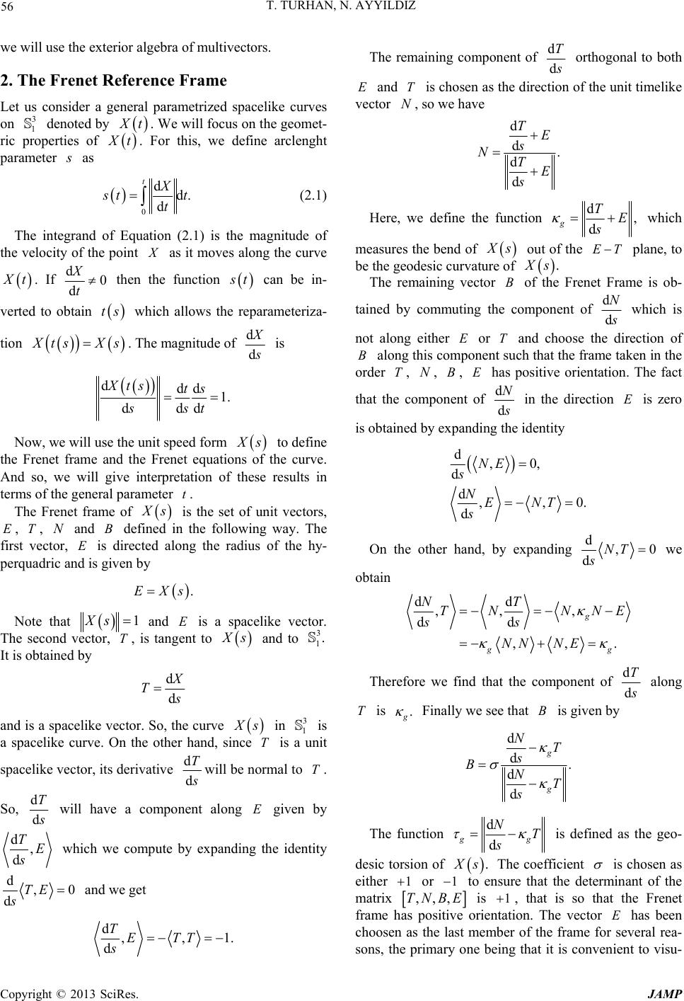 T. TURHAN, N. AYYILDIZ 56 we will use the exterior algebra of multivectors. 2. The Frenet Reference Frame Let us consider a general parametrized spacelike curves on denoted by 3 1 t . We will focus on the geomet- ric properties of t. For this, we define arclenght parameter as 0 dd. d tX t t t (2.1) The integrand of Equation (2.1) is the magnitude of the velocity of the point as it moves along the curve X t. If d0 d X t then the function t can be in- verted to obtain ts which allows the reparameteriza- tion ts Xs. The magnitude of d d is ddd 1. ddd Xts ts sst Now, we will use the unit speed form s to define the Frenet frame and the Frenet equations of the curve. And so, we will give interpretation of these results in terms of the general parameter . t The Frenet frame of s is the set of unit vectors, , , and TN defined in the following way. The first vector, is directed along the radius of the hy- perquadric and is given by .EXs Note that 1Xs and is a spacelike vector. The second vector, , is tangent to T s and to It is obtained by 3 1. d d T and is a spacelike vector. So, the curve sT in is a spacelike curve. On the other hand, since is a unit 3 1 spacelike vector, its derivative d d T will be normal to . So, T d d T will have a component along given by d, d TE s which we compute by expanding the identity d, dTE s0 and we get d,, d TETT s The remaining component of d d T orthogonal to both and T is chosen as the direction of the unit timelike vector , so we have N d d. d d TE s NTE s Here, we define the function d, d gTE s which measures the bend of s out of the T plane, to be the geodesic curvature of . s The remaining vector of the Frenet Frame is ob- tained by commuting the component of d d N which is not along either or and choose the direction of T along this component such that the frame taken in the order , , TN , has positive orientation. The fact that the component of d d N in the direction is zero is obtained by expanding the identity d,0, d d,, d NE s NENT s 0. On the other hand, by expanding d, dNT s0 we obtain dd ,, , dd ,, g gg NT TN NN ss NN NE . E Therefore we find that the component of d d T along is T. Finally we see that is given by d d. d d g g NT s BNT s The function d d g NT s g is defined as the geo- desic torsion of . s The coefficient is chosen as either 1 or 1 to ensure that the determinant of the matrix ,,TN ,EB is 1 , that is so that the Frenet frame has positive orientation. The vector has been choosen as the last member of the frame for several rea- sons, the primary one being that it is convenient to visu- 1. Copyright © 2013 SciRes. JAMP 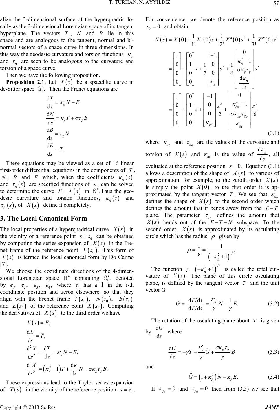 T. TURHAN, N. AYYILDIZ 57 alize the 3-dimensional surface of the hyperquadric lo- cally as the 3-dimensional Lorentzian space of its tangent hyperplane. The vectors T, and N lie in this space and are analogous to the tangent, normal and bi- normal vectors of a space curve in three dimensions. In this way the geodesic curvature and torsion functions and are seen to be analogous to the curvature and torsion of a space curve. Then we have the following proposition. Proposition 2.1. Let s be a spacelike curve in de-Sitter space Then the Frenet equations are 3 1. d d d d d d d. g gN d T s NTB s B s ET s gg NE These equations may be viewed as a set of 16 linear first-order differential equations in the components of , , T N and which, when the coefficients g and g are specified functions of , can be solved to determine the curve EXs in Thus the geo- desic curvature and torsion functions, 3 1. g and g , of s define it completely. 3. The Local Canonical Form The local properties of a hyperquadrical curve s in the vicinity of a reference point 0 s can be obtained by computing the series expansion of s in the Fre- net frame of the reference point 0. s This form of s ,e is termed the local canonical form by Do Carmo [7]. We choose the coordinate directions of the 4-dimen- sional Lorentzian space containing denoted by 1 2 3 4 where i has a in the i-th coordinate position and zeros elsewhere, so that they align with the Frenet frame 4 1 3 1, 1 ,e,e,e e 0,Ts Ns 0, 0 Bs and 0 Es of the reference point 0. s Computing the derivatives of s to the third order we have 2 2 3 2 3 , d, d dd , 1TN s d d d d g ggg Xs E XT s XT NE s s XB s dd . These expressions lead to the Taylor series expansion of s in the vicinity of the reference position 0 s . For convenience, we denote the reference position as 00s and obtain 0 0 23 2 23 2 2 11 1 00 00 1! 2!3! 0 1 10 1 0 01 11 0 00 26 d 00 d 0 1 10 1 0 01 0 00 2 00 g gg g g g g sXX sXsXs ss s s s s 00 1 3 6 gg g s (3.1) where 0 and 0 are the values of the curvature and torsion of s and 1 is the value of d d , all evaluated at the reference position Equation (3.1) allows a description of the shape of 0.s s to various of approximation, for example, to the zeroth order s is simply the point 0X, to the first order it is ap- proximated by the tangent vector . We see that 0 T defines the shape of s to the second order which defines the amount that it bends away from the T plane. The parameter 0 defines the amount that s bends out of the subspace. To the second order, ETN s is approximated by its osculating circle which has the radius given by 12 2 11 . 1 g The function 12 21 g is called the total cur- vature of . s The plane of this circle osculating plane, is defined by the tangent vector and the unit vector G T dd 1 . dd g Ts GN Ts E (3.2) The rotation of the osculating plane about is given by T d d G where d d ggg GTG s B (3.3) and 2 1 gg GN .E (3.4) If 10 g and 00 g then from (3.3) we see that Copyright © 2013 SciRes. JAMP 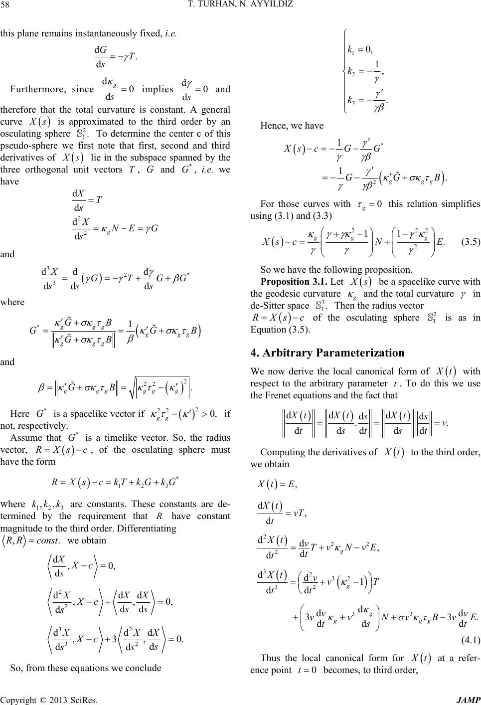 T. TURHAN, N. AYYILDIZ 58 this plane remains instantaneously fixed, i.e. d. d GT s Furthermore, since d0 d g s implies d0 ds and therefore that the total curvature is constant. A general curve s is approximated to the third order by an osculating sphere To determine the center c of this pseudo-sphere we first note that first, second and third derivatives of 2 1. s lie in the subspace spanned by the three orthogonal unit vectors T, and , i.e. we have G* G 2 2 d d d dg XT s XNE G s and 3 2* 3 dd d dd d XGTG ss s G where *1 gggggg ggg GB G G GB B and 2 22 . gggggg GB Here is a spacelike vector if if not, respectively. * G 2 22 0, gg Assume that is a timelike vector. So, the radius vector, , of the osculating sphere must have the form * G sRX c * 123 RXsckTkGkG where 123 are constants. These constants are de- termined by the requirement that ,,kkk have constant magnitude to the third order. Differentiating ,const.RR we obtain 2 2 32 32 d,0, d ddd ,, dd d ddd ,3, d dd XXc s XXX Xc ss s XX Xc s ss 0, 0. X So, from these equations we conclude 1 2 3 0, 1, . k k k Hence, we have * 2 1 1. ggg Xs cGG GG B For those curves with 0 g this relation simplifies using (3.1) and (3.3) 22 2 11 . ggg 2 scN E (3.5) So we have the following proposition. Proposition 3.1. Let s be a spacelike curve with the geodesic curvature and the total curvature in de-Sitter space Then the radius vector 3 1. RXsc of the osculating sphere is as in Equation (3.5). 2 1 4. Arbitrary Parameterization We now derive the local canonical form of t with respect to the arbitrary parameter . To do this we use the Frenet equations and the fact that t dd d dd .. ddddd Xt XtXt ss v tstst Computing the derivatives of t to the third order, we obtain 2 22 2 3232 32 33 , d, d dd, d d dd1 dd d dd 33 dd d g g g ggg XtE Xt vT t Xt vTvNvE t t Xt vvT tt vv vvNvBv ts .E t (4.1) Thus the local canonical form for t at a refer- ence point 0t becomes, to third order, Copyright © 2013 SciRes. JAMP  T. TURHAN, N. AYYILDIZ Copyright © 2013 SciRes. JAMP 59 0 00 01 0 23 2 23 2 232 2 2 3 2 3 1d 1d1d 00 00 1! d2!3! dd d 3d 10 d d1 01 d d. 00 26 0 00 d d 3dd g gg gg g XX X 3 3 tXt tt ttt v vt vv vv t t t tv vv vv ts 6. Conclusion t This work develops the differential geometry of space- like curves on de-Sitter space in four-dimensional Lor- entzian space. The motivation for this work is the fact that the Euler parameters of spherical displacements can be used to map them to points on 3 1. REFERENCES [1] B. O’Neill, “Semi-Riemann Geometry: With Applictions to Relativity,” Academic Press, New York, 1983, 469 p. 5. Formula for Geodesic Curvature and Torsion [2] T. Fusho and S. Izumiya, “Lightlike Surfaces of Space- like Curves in de Sitter 3-Space,” Journal of Geometry, Vol. 88, 2008, pp. 19-29. http://dx.doi.org/10.1007/s00022-007-1944-5 We now compute the vector 2 2 dd dd XX tt which in view of Equation (4.1) becomes [3] M. Kasedou, “Singularities of Lightcone Gauss Images of Spacelike Hypersurfaces in de Sitter Space,” Journal of Geometry, Vol. 94, 2009, pp. 107-121. http://dx.doi.org/10.1007/s00022-009-0001-y 2 3 2 dd . ddg XX vTNE tt (5.1) [4] J. M. McCarthy, “The Differential Geometry of Curves in an Image Space of Spherical Kinematics,” Mechanism and Machine Theory, Vol. 22, No. 3, 1987, pp. 205-211. http://dx.doi.org/10.1016/0094-114X(87)90003-6 Computing the scalar product of (5.1) with itself, we obtain the following equation for the geodesic curvature : [5] J. M. McCarthy and B. Ravani, “Differential Kinematics of Spherical and Spatial Motions Using Kinematic Map- ping,” Journal of Applied Mechanics, Vol. 53, No. 1, 1986, pp. 15-22. http://dx.doi.org/10.1115/1.3171705 22 22 2 3 dd dd , dd dd . dd , dd g XX XX X tt tt XX tt [6] B. Ravani and B. Roth, “Mappings of Spatial Kinemat- ics,” Journal of Mechanisms, Transmissions and Automa- tion in Design, Vol. 106, No. 3, 1984, pp. 341-347. http://dx.doi.org/10.1115/1.3267417 And a formula for geodesic torsion can be given as 23 22 dd d det,,,. ddd g g3 XX Ettt [7] M. P. Do Carmo, “Differential Geometry of Curves and Surfaces,” Prentice-Hall, Englewood Cliffs, 1976, 503 p. This relation can be also seen in [2].
|