 Journal of Applied Mathematics and Physics, 2013, 1, 47-54 http://dx.doi.org/10.4236/jamp.2013.13008 Published Online August 2013 (http://www.scirp.org/journal/jamp) Investigation of the Appropriate Partial Level Density Formula for Pre-Equilibrium Nuclear Exciton Model Shafik Shakir Shafik1*, Ali Dawoud Salloum2 1Department of Physics, College of Science, University of Baghdad, Baghdad, Iraq 2Department of Physics, College of Science for Women, University of Baghdad, Baghdad, Iraq Email: *shafeq_sh@yahoo.com Received June 10, 2013; revised July 15, 2013; accepted August 20, 2013 Copyright © 2013 Shafik Shakir Shafik, Ali Dawoud Salloum. This is an open access article distributed under the Creative Com- mons Attribution License, which permits unrestricted use, distribution, and reproduction in any medium, provided the original work is properly cited. ABSTRACT Ericson formula represents the first formula, which was suggested to describe the partial level density (PLD) formula in pre-equilibrium region of the nuclear reactions. Then a number of corrections were added to this formula in order to make it more suitable to physical meaning. In this paper, there are two aims to be done: the first aim is to study the cor- respondence between one and two-components formulae in Ericson, Pauli, and pairing corrections; the second aim is to compare and study the results of Comprehensive formula, which contents with all corrections, with Ericson, Pauli, and pairing formulae. The Comprehensive formula was suggested to simulate the reality. To achieve these aims the 56Fe and 90Zr nuclei were chosen and the results showed that the difference between one and two-components formulae was too small which can be neglected. Furthermore, the results strongly recommended that for cross section calculations of the nuclear reaction, one must use Comprehensive formula rather than Pauli formula. Keywords: Partial Level Density; Pre-Equilibrium Model; Nuclear Reaction; Exciton Model; Equidistant Spacing Model; 56Fe; 90Zr 1. Introduction Nuclear reactions are divided according to the energy of the incident particle to low, medium, and high-energy reactions. Pre-Equilibrium (PE) region is a stage in nu- clear reaction, which represents the case when the ex- citation energy is not distributed equally between the nu- cleons of the excited nucleus. Many models describe this region such as: the Intra-Nuclear-Cascade (INC) model [1], the Harp-Miller-Berne (HMB) model [2,3], the Hybrid model [4], the Geometry Dependent Hybrid model [5] and the Exciton model [6]. J. J. Griffin sug- gested the Exciton model at 1966 [6]. It was preferred model by many researchers [7,8] because it is simplest in the description and treatment of the PE nuclear emission. The idea of this model supposes that when the bom- barding particle hit the target nucleus, it begins to share its energy with the first particle collides with it, then by successive nucleon-nucleon interactions in a series of stages and before attend to the complete interactions (equi- librium), the nuclear emission occurs. Each interaction produces a particle-hole (p-h) pair, and the sum of such particle and hole called an Exciton. The first few states are 2p 1h, 3p 2h and so on. The numbers of excitons are n (n = p + h) and the stages are labeled by s so that n = 2s + 1, therefore, again, through exciton production, the nuclear emission may occur [9]. 2. The Partial Level Density (PLD) The PLD represents important quantity in nuclear phys- ics. It is used in calculation of cross section, double dif- ferential cross section and transition rates [9,10]. PLD can be measured experimentally up to 15 MeV; above this value of energy, the levels converge. Therefore, the spacing between them overlapped, and it is difficult to calculate them. Hence, level density may be calculated by theoretical methods [8-10]. In this paper, the theo- retical description of PLD by the exciton model was de- pended and developed through many stages. The Fermi gas model (FGM) was used as description model in the nuclear reaction exciton model. FGM conceder equal spaces between the levels and this called Equidistant Spacing Model (ESM) [9,10]. *Corresponding author. C opyright © 2013 SciRes. JAMP 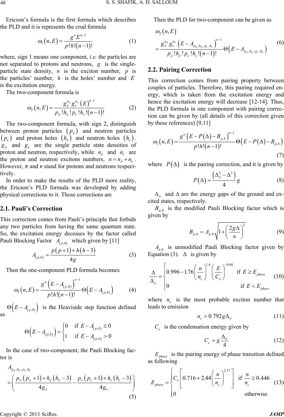 S. S. SHAFIK, A. D. SALLOUM 48 Ericson’s formula is the first formula which describes the PLD and it is represents the crud formula 1 1,!! 1! nn gE nE ph n (1) where, sign 1 means one component, i.e. the particles are not separated to protons and neutrons, is the single- particle state density, is the exciton number, is the particles’ number, is the holes’ number and is the excitation energy. n hpE The two-component formula is 1 2,!!!!1! n nn gg E nE phphn (2) The two-component formula, with sign 2, distinguish between proton particles p and neutron particles p and proton holes h and neutron holes h . and are the single particle state densities of proton and neutron, respectively, while n and n are the proton and neutron excitons numbers, nnn . However, ߨ and v stand for protons and neutrons respect- tively. In order to make the results of the PLD more reality, the Ericson’s PLD formula was developed by adding physical corrections to it. Those corrections are 2.1. Pauli’s Correction This correction comes from Pauli’s principle that forbids any two particles from having the same quantum state. So, the excitation energy deceases by the factor called Pauli Blocking Factor , h A which given by [11] , 13 4 ph pp hh Ag (3) Then the one-component PLD formula becomes 1 , 1, ,!! 1! n nph ph gEA nEE A ph n (4) ,ph EA is the Heaviside step function defined as , , , 0if 0 1if 0 ph ph ph EA EA EA In the case of two-component, the Pauli Blocking fac- tor is ,,, 13 1 44 phph A pphhpphh gg Then the PLD for two-component can be given as 2 1 ,, , , ,, , Θ !!!!1! n nn phph phph nE gg EAEA phphn (6) 2.2. Pairing Correction This correction comes from pairing property between couples of particles. Therefore, this pairing required en- ergy, which is taken from the excitation energy and hence the excitation energy will decrease [12-14]. Thus, the PLD formula in one component with pairing correc- tion can be given by (all details of this correction given by these references) [9,11] 1 , 1 , ,Θ !! 1! n nph h gEP B nEE PB ph n (7) where P is the pairing correction, and it is given by 22 4 P g (8) and ∆ are the energy gaps of the ground and ex- cited states, respectively. , h is the modified Pauli Blocking factor which is given by B 2 ,, 2 1 ph phg BA n (9) ,ph is unmodified Pauli Blocking factor given by Equation (3). A is given by 1.6 0.68 0.996 1.76if 0i phase ce f hase nE EE nC EE (10) where c is the most probable exciton number that leads to emission n 0.792 c n (11) e C is the condensation energy given by 4 e Cg (12) phase is the pairing energy of phase transition defined as following E 3 (5) 2.17 0.716 2.44if0.446 0o e phase cc nn C Enn therwise (13) Copyright © 2013 SciRes. JAMP 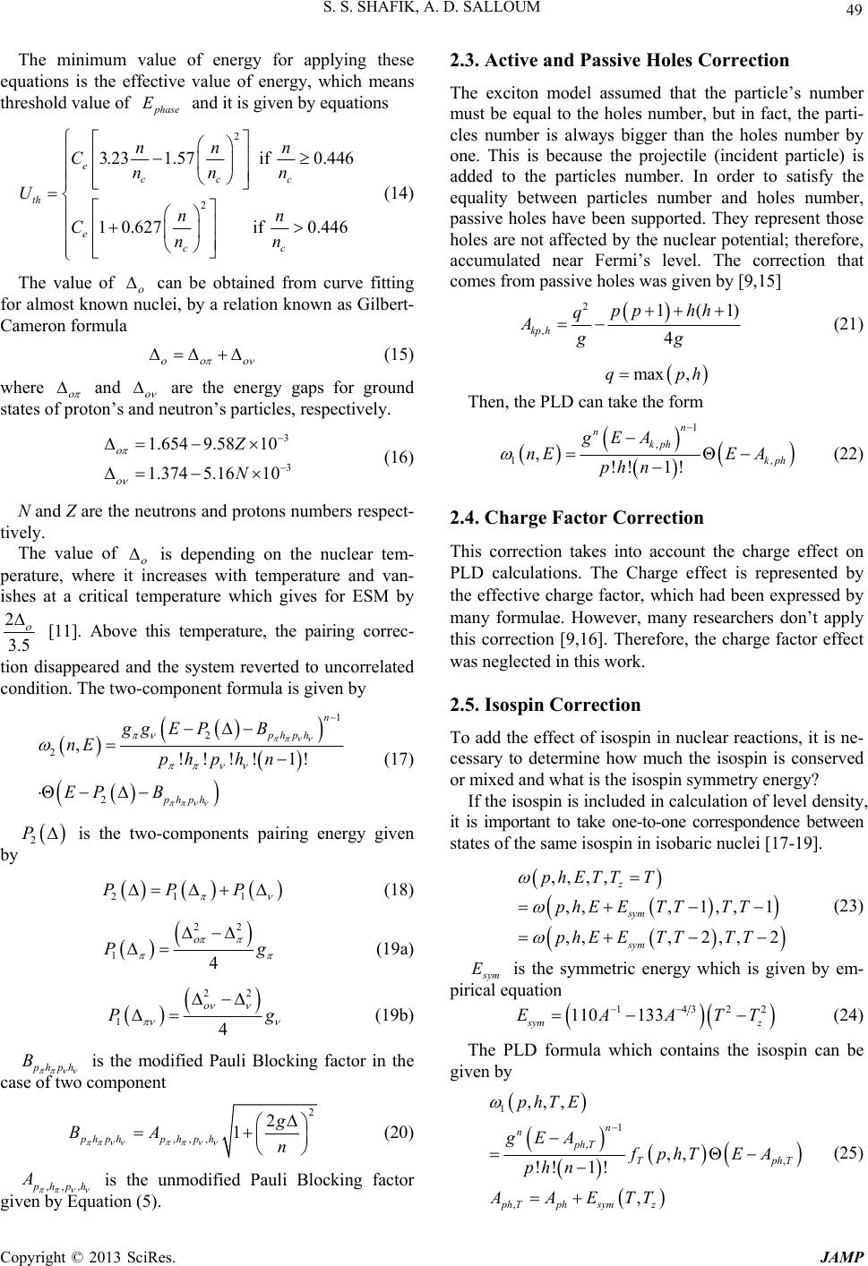 S. S. SHAFIK, A. D. SALLOUM 49 The minimum value of energy for applying these equations is the effective value of energy, which means threshold value of and it is given by equations phase E 2 2 if 0.446 1if 3.23 1.57 4460.627 eccc th ecc nnn Cnnn Unn Cnn 0. (14) The value of can be obtained from curve fitting for almost known nuclei, by a relation known as Gilbert- Cameron formula (15) where and are the energy gaps for ground states of proton’s and neutron’s particles, respectively. 3 3 11.654 9.58 1.374 5.16 0 10 Z N (16) N and Z are the neutrons and protons numbers respect- tively. The value of is depending on the nuclear tem- perature, where it increases with temperature and van- ishes at a critical temperature which gives for ESM by 2 3.5 [11]. Above this temperature, the pairing correc- tion disappeared and the system reverted to uncorrelated condition. The two-component formula is given by 1 2 2 2 ,!!!! 1! Θ n phph phph ggE PB nE phphn EP B (17) 2 P is the two-components pairing energy given by 21 1 PP P (18) 22 14 P g (19a) 22 14 g (19b) hph B is the modified Pauli Blocking factor in the case of two component 2 ,,, 2 1 phphphphg BA n (20) ,,, hph A is the unmodified Pauli Blocking factor given by Equation (5). 2.3. Active and Passive Holes Correction The exciton model assumed that the particle’s number must be equal to the holes number, but in fact, the parti- cles number is always bigger than the holes number by one. This is because the projectile (incident particle) is added to the particles number. In order to satisfy the equality between particles number and holes number, passive holes have been supported. They represent those holes are not affected by the nuclear potential; therefore, accumulated near Fermi’s level. The correction that comes from passive holes was given by [9,15] 2 , 1(1 4 kp h pp hh q Agg ) (21) max ,qph Then, the PLD can take the form 1 , 1, ,Θ !! 1! n nkph kph gEA nEE A ph n (22) 2.4. Charge Factor Correction This correction takes into account the charge effect on PLD calculations. The Charge effect is represented by the effective charge factor, which had been expressed by many formulae. However, many researchers don’t apply this correction [9,16]. Therefore, the charge factor effect was neglected in this work. 2.5. Isospin Correction To add the effect of isospin in nuclear reactions, it is ne- cessary to determine how much the isospin is conserved or mixed and what is the isospin symmetry energy? If the isospin is included in calculation of level density, it is important to take one-to-one correspondence between states of the same isospin in isobaric nuclei [17-19]. ,, ,, ,,, 1,, 1 ,,, 2,, 2 z sym sym phETT T phEETTTT phE ETTTT (23) ym is the symmetric energy which is given by em- pirical equation E 1432 1310 31 sym z EAAT 2 T (24) The PLD formula which contains the isospin can be given by 1 1 , , , ,,, ,, Θ !! 1! , n nph T Tp ph Tphsymz phTE gEAfphT EA ph n AAETT hT (25) Copyright © 2013 SciRes. JAMP  S. S. SHAFIK, A. D. SALLOUM 50 ,, T phT T is the correction factor of states with good isospin. If isospin is assumed to be completely mixed, the symmetric energy is zero and the correction factor is unity. 2.6. Spin Correction Spin effect is also added to the PLD formula as a correc- tion and it is assumed factorized [20-23] 1 , , Θ !! 1 ,! , n nph nph gEARJ EA p Jhn nE (26) 2 2 3 1 21 2 exp 2 22 n n J J RJ (27) n is the spin cut off parameter. It is important to mention that Equation (26) used for pre-compound nu- cleus and it does not use for compound nucleus [22]. 2 0.16 nn23 (28) 2.7. Surface Correction The initial interaction between a projectile and target nucleon is frequently localized near the nucleus surface. Since the nuclear density variant with nuclear radius, hence the nuclear potential is shallower than in the inte- rior; therefore, the local well depth (i.e. near the surface) is less the central depth [9,11,24]. This must add a con- siderable effect on PLD calculations especially in the exciton knockout and pickup nuclear reactions. If we labeled ,,nEV as the PLD of one-com- ponent Fermi gas system with exciton number exci- tation energy and nuclear potential well depth V, then one can write the following equation for PLD with surface effect ,n E 111 ,,,, ,,nEVnEf nEV (29) where 1,,nE is the PLD calculated for V , and it is given by the simple one-component PLD Pauli formula (Equation (4)) 1 , 1 ,, Θ !! 1! n nph , h gEA nEE A ph n (30) The function 1,, nEV in Equation (29) is the cor- rection due to surface effect in the ESM, and it is given by 1 10 ,, 1 n j hh j j EjVh fnEVC E From Equation (29), the PLD formula was corrected to in (31) clude the finite well depth and then was extended to include correction due to surface effect. This was done in the initial particle-nucleus interaction by replacing the nuclear potential depth 0 V by 1 V. This means instead of putting 0 VV , we put 1 VV. The new potential depth 1 V, ined as therage effective well depth”he choice between is defe “av . T1 V and 0 V is 0 1 38 MV1Vhe 0 VVh For (n, n) reaction 1, 7MeV nn V [24]. 3. Comprehensive Formula includes all the pre- Comprehensive formula is a formula vious corrections, except the isospin correction because the reaction was assumed to be completely mixed [17,18], then the isospin correction became unity. The aim behind suggested this formula is an attempt to get on a formula describes the PE PLD by the most accurate description (real one). 1 ,, 11 ,,, , !! 1! n nph kph gEPB A phEf nEV ph n ,, Θ np RJ EPBA hkph (32) 4. Results and Discussion be calculated experi- 4.1. Comparison between One and In orrence between one and two- It is obvious that the PLD cannot mentally especially for excitation energy more than 15 MeV because the states overlapped with each other’s. On the other hand, and in order to increasing knowledge about the nuclear force, which represents the strongest force comparing with others, one must increase the ap- plied excitation energy to hundred and several hundred MeVs. Therefore, PLD must be given in theoretical form. The calculated Comprehensive formula (Equation (32)) is a suitable formula for PLD estimations. This claim can be examined if one applies the Comprehensive formula of the PLD in cross section equation of any (and for any nucleus) PE nuclear models and comparing with experi- mental results of this cross section. However, PLD for- mula with Pauli’s correction was used in cross section calculations by many researchers [25-27] and these re- searchers avoided use all corrections of the PLD to ease the programming potential. Further, in these results, Pauli’s correction was stand as a reference case for PLD comparisons with all their corrections. Two-Component der to study the diffe component formulae of the PLD, a comparison was made Copyright © 2013 SciRes. JAMP  S. S. SHAFIK, A. D. SALLOUM Copyright © 2013 SciRes. JAMP 51 for 56Fe isotope. All used parameter are listed in Tabl e 1. From Figures 1(a)-(c) one can see that the two-compo- nent results are less than those of one-component. This behavior is expected physically because the two-com- ponent system will have to share the energy with more entities (the entities are those due to particles and holes of the neutrons and protons). Although the neutron parti- cles and holes are considered zero, the two component results stay less than the one-component results. From Figures 1(a)-(c) one can see that the two-com- ponent results are less than those of one-component. This behavior is expected physically because the two-com- ponent system will have to share the energy with more entities (the entities are those due to particles and holes Figure 1. (a) One and two-components Ericson’s formulae of PLD for 56Fe isotope; (b) One and tw-components Pauli’s for- o mulae of PLD of 56Fe isotope; (c) One and two-components pairing formulae of PLD for 56Fe isotope.  S. S. SHAFIK, A. D. SALLOUM 52 f the neutrons and protons). Although the neutron parti- of the 56Fe isotope because the mo cles and holes are considered zero, the two component results stay less than the one-component results. In addition, it is noted from Figures 1(a)-(c) and Ta- bl 4.2. Behavior of One-Component Corrections all approximately sa at ass number is higher e 2 that the ratio between one and two-components results is small for main forms of the PLD formulae (Ericson, Pauli, and Pairing PLD formulae), therefore, one-component formula may be used instead of two- component formula with acceptable results. The PLD of one-component for Ericson formula with corrections for 56Fe isotope can be shown in Figure 2. It is noted from this figure that the arrangement of the re- sults from bottom to top is surface correction, Pauli’s correction, Ericson’s correction, pairing correction, spin correction, active and passive correction and Compre- hensive formula, respectively. Whereas, for 90Zr isotope, shown in Figure 3, the arrangement is surface correction, Pauli correction, Ericson’s correction, spin correction, active and passive holes correction, pairing correction and Comprehensive formula, respectively. The results of these two figures give me arrangements. As we mentioned above, if one used PLD with Pauli correction as reference, then it is easy to see that except surface correction, the all corrections and Comprehensive PLD formulae have values more than PLD with Pauli correction. However, one can expect that the use of PLD formula with Pauli correction alone in cross section calculations may deviate the theoretical estimations from experimental results. Therefore, these results strongly suggested that the Comprehensive PLD formulae must be used in any calculations need PLD. Finally, the results of 90Zr isotope are bigger than th and then the single particle level density increases. On the other hand, the difference between the results decreases with increasing the excitation energy. 5. Conclusion ents in nuclear reaction and Table 1. The parameter used in the present calculations. T PLD represents mean argum stricture models. This paper submitted a good literature arget nucleus under investigation 56Fe Mass number 56 Ato Neutr Exciton configuration (3,3) for onmponent (3t Max. excitation energy mic number26 ons number 30 Exciton number 6 e-co ,3,0,0) for two-componen 100MeV Single particle density A/13 able 2. The ratio between one and two-component formu- The correction two and one T lae for Ericson, Pauli and pairing PLD. The ratio between components 21 Ericson 0.007 Pauli 0.015 Pairing 0.02 Figure 2. PLD of one-component with all corrections for 56Fe isotope. Copyright © 2013 SciRes. JAMP 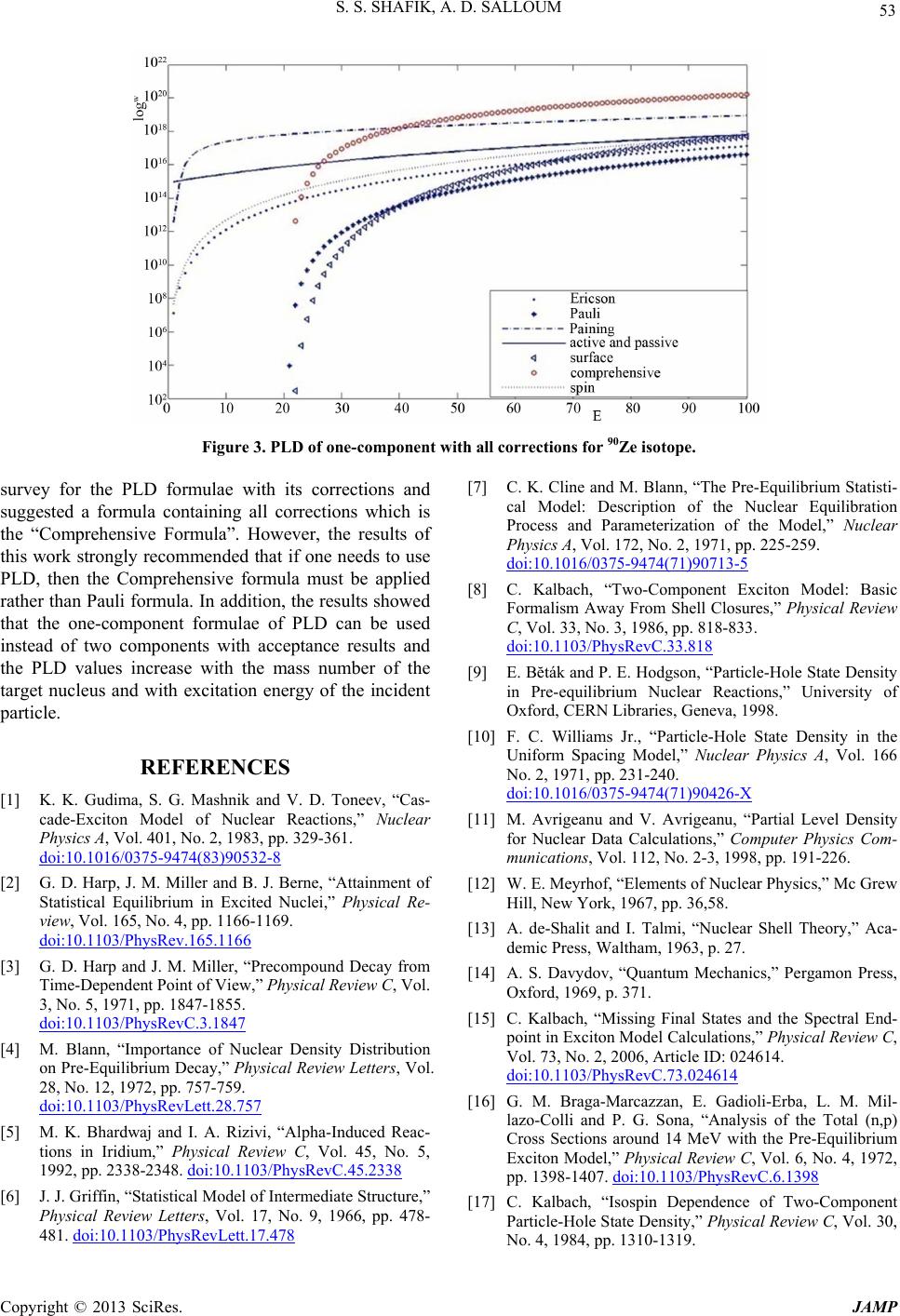 S. S. SHAFIK, A. D. SALLOUM 53 Figure 3. PLD of one-component with all corrections for 90Ze isotope. rvey for the PLD formulae with its corrections and REFERENCES [1] K. K. Gudima D. Toneev, “Cas- [7] C. K. Cline and M. Blann, “The Pre-Equilibrium Statisti- su suggested a formula containing all corrections which is the “Comprehensive Formula”. However, the results of this work strongly recommended that if one needs to use PLD, then the Comprehensive formula must be applied rather than Pauli formula. In addition, the results showed that the one-component formulae of PLD can be used instead of two components with acceptance results and the PLD values increase with the mass number of the target nucleus and with excitation energy of the incident particle. , S. G. Mashnik and V. cade-Exciton Model of Nuclear Reactions,” Nuclear Physics A, Vol. 401, No. 2, 1983, pp. 329-361. doi:10.1016/0375-9474(83)90532-8 [2] G. D. Harp, J. M. Miller and B. J. Berne, “Attainment of Statistical Equilibrium in Excited Nuclei,” Physical Re- view, Vol. 165, No. 4, pp. 1166-1169. doi:10.1103/PhysRev.165.1166 [3] G. D. Harp and J. M. Miller, “Precompound Decay from Time-Dependent Point of View,” Physical Review C, Vol. 3, No. 5, 1971, pp. 1847-1855. doi:10.1103/PhysRevC.3.1847 [4] M. Blann, “Importance of Nuclear Density Distribution on Pre-Equilibrium Decay,” Physical Review Letters, Vol. 28, No. 12, 1972, pp. 757-759. doi:10.1103/PhysRevLett.28.757 [5] M. K. Bhardwaj and I. A. Rizivi, “Alpha-Induced Reac- tions in Iridium,” Physical Review C, Vol. 45, No. 5, 1992, pp. 2338-2348. doi:10.1103/PhysRevC.45.2338 [6] J. J. Griffin, “Statistical Model of Intermediate Structure,” Physical Review Letters, Vol. 17, No. 9, 1966, pp. 478- 481. doi:10.1103/PhysRevLett.17.478 cal Model: Description of the Nuclear Equilibration Process and Parameterization of the Model,” Nuclear Physics A, Vol. 172, No. 2, 1971, pp. 225-259. doi:10.1016/0375-9474(71)90713-5 [8] C. Kalbach, “Two-Component Exciton Model: Basic Formalism Away From Shell Closures,” Physical Review C, Vol. 33, No. 3, 1986, pp. 818-833. doi:10.1103/PhysRevC.33.818 [9] E. Bĕták and P. E. Hodgson, “Particle-Hole State Density Density in the 0426-X in Pre-equilibrium Nuclear Reactions,” University of Oxford, CERN Libraries, Geneva, 1998. [10] F. C. Williams Jr., “Particle-Hole State Uniform Spacing Model,” Nuclear Physics A, Vol. 166 No. 2, 1971, pp. 231-240. doi:10.1016/0375-9474(71)9 artial Level Density w Shell Theory,” Aca- cs,” Pergamon Press, Final States and the Spectral End- [11] M. Avrigeanu and V. Avrigeanu, “P for Nuclear Data Calculations,” Computer Physics Com- munications, Vol. 112, No. 2-3, 1998, pp. 191-226. [12] W. E. Meyrhof, “Elements of Nuclear Physics,” Mc Gre Hill, New York, 1967, pp. 36,58. [13] A. de-Shalit and I. Talmi, “Nuclear demic Press, Waltham, 1963, p. 27. [14] A. S. Davydov, “Quantum Mechani Oxford, 1969, p. 371. [15] C. Kalbach, “Missing point in Exciton Model Calculations,” Physical Review C, Vol. 73, No. 2, 2006, Article ID: 024614. doi:10.1103/PhysRevC.73.024614 [16] G. M. Braga-Marcazzan, E. Gadioli-Erba, L. M. Mil- lazo-Colli and P. G. Sona, “Analysis of the Total (n,p) Cross Sections around 14 MeV with the Pre-Equilibrium Exciton Model,” Physical Review C, Vol. 6, No. 4, 1972, pp. 1398-1407. doi:10.1103/PhysRevC.6.1398 [17] C. Kalbach, “Isospin Dependence of Two-Component Particle-Hole State Density,” Physical Review C, Vol. 30, No. 4, 1984, pp. 1310-1319. Copyright © 2013 SciRes. JAMP  S. S. SHAFIK, A. D. SALLOUM 54 doi:10.1103/PhysRevC.30.1310 density with Good Iso-[18] C. Kalbach, “Particle-Hole State spin,” Physical Review C, Vol. 47, No. 2, 1993, pp. 587- 601. doi:10.1103/PhysRevC.47.587 [19] C. Kalbach, “Isospin Conversion in Preequilibrium Reac- tions,” Physical Review C, Vol. 72, No. 2, 2005, Article ID: 024607. doi:10.1103/PhysRevC.72.024607 [20] C. Kalbach and F. M. Mann, “Phenomenology of Con- tinuum Angular Distributions. I. Systematics and Para- metrization,” Physical Review C, Vol. 23, No. 1, 1981, pp. 112-123. doi:10.1103/PhysRevC.23.112 [21] C. Kalbach, “Phenomenology of Continuum Angular Distributions. II. Griffin Preequilibrium Model,” Physical Review C, Vol. 23, No. 1, pp. 124-135. doi:10.1103/PhysRevC.23.124 [22] M. B. Chadwick and P. Obložinský, “Particle-Hole State Densities with Linear Momentum and Angular Distribu- tions in Preequilibrium Reaction,” Physical Review C, Vol. 46, No. 5, 1992, pp. 2028-2041. doi:10.1103/PhysRevC.46.2028 [23] S. S. Shafik, “Angular Momentum Distribution for State M. Kolomietz, A. I. Sanzhur and S. Density with Non-ESM Dependence,” Journal of Fisica Nucleare, 2009. [24] Ye. A. Bogila, V. Shlomo, “Preequilibrium Decay in the Exciton Model for Nuclear Potential with a Finite Depth,” Physical Review C, Vol. 53, No. 2, 1996, pp. 855-859. doi:10.1103/PhysRevC.53.855 [25] M. Avrigeanu, A. Harangozo and V. Avrigeanu, “Aver- age Strength of the Effective Interaction in Multistep Di- rect Reactions,” Physical Review C, Vol. 56, No. 3, 1997, pp. 1633-1636. doi:10.1103/PhysRevC.56.1633 [26] Y. K. Gupta, D. C. Biswas, Bency John, B. K. Nayak, A. Saxena and R. K. Choudhury, “Nuclear Level-Density Parameters of Nuclei in the Z~70 and A~180 Mid-Shell Regions,” Physical Review C, Vol. 80, No. 5, 2009, Arti- cle ID: 054611. doi:10.1103/PhysRevC.80.054611 [27] H. Nakada and Y. Alhassid, “Publisher’s Note: Iso- spin-Projected Nuclear Level Densities by the Shell Mo- del Monte Carlo Method,” Physical Review C, Vol. 78, No. 6, 2008, Article ID: 069907. doi:10.1103/PhysRevC.78.069907 Copyright © 2013 SciRes. JAMP
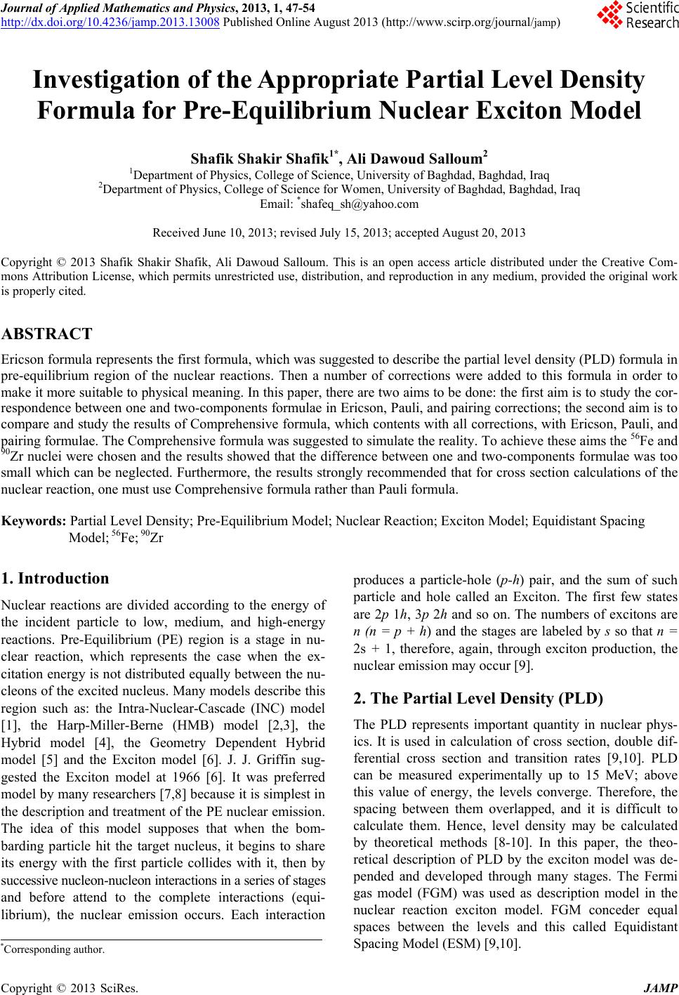
|