Applied Mathematics, 2013, 4, 1347-1360
http://dx.doi.org/10.4236/am.2013.49182 Published Online September 2013 (http://www.scirp.org/journal/am)
A Closed-Form Approximation for Pricing
Temperature-Based Weather
Derivatives
A. E. Clements, A. S. Hurn, K. A. Lindsay
School of Economics and Finance, Queensland University of Technology, Brisbane, Australia
Received May 22, 2013; revised June 22, 2013; accepted June 30, 2013
Copyright © 2013 A. E. Clements et al. This is an open access article distributed under the Creative Commons Attribution License,
which permits unrestricted use, distribution, and reproduction in any medium, provided the original work is properly cited.
ABSTRACT
This paper develops analytical distributions of temperature indices on which temperature derivatives are written. If the
deviations of daily temperatures from their expected values are modelled as an Ornstein-Uhlenbeck process with time-
varying variance, then the distributions of the temperature index on which the derivative is written is the sum of trun-
cated, correlated Gaussian deviates. The key result of this paper is to provide an analytical approximation to the distri-
bution of this sum, thus allowing the accurate computation of payoffs without the need for any simulation. A data set
comprising average daily temperature spanning over a hundred years for four Australian cities is used to demonstrate
the efficacy of this approach for estimating the payoffs to temperature derivatives. It is demonstrated that expected pay-
offs computed directly from historical records are a particularly poor approach to the problem when there are trends in
underlying average daily temperature. It is shown that the proposed analytical approach is superior to historical pricing.
Keywords: Weather Derivatives; Temperature Models; Cooling-Degree Days; Distributions for Correlated Variables
1. Introduction
A weather derivative takes its value from an underlying
measure of weather, such as temperature, rainfall or
snowfall over a particular period of time, and permits the
financial risk associated with climatic conditions to be
managed. Major participants in this market include utili-
ties and insurance companies along with other firms with
costs or revenues that are dependent upon the weather.
For example, an electricity supplier normally provides its
customers with electricity at a fixed price irrespective of
the wholesale price. On the other hand the wholesale
price of electricity can fluctuate wildly with extreme
temperatures, and so temperature-based derivatives can
provide a hedging tool for fluctuations in wholesale elec-
tricity prices. The first weather derivative was transacted
in the US in 1996 and the size of the market now exceeds
US$ 8 billion. Almost all weather derivatives are based
on temperature indices such as heating degree days and
cooling degree days and consequently the focus of this
paper will be exclusively on developing closed-form ap-
proximations to the distribution of the temperature indi-
ces on which temperature-based derivatives are written
which in turn affects their valuation1.
Traditionally, the valuation of options discounts the
expected payoff at the risk-free force of interest based on
a zero-arbitrage argument involving the formation of a
portfolio consisting of a risk-free combination of an op-
tion and the underlying asset [3]. Because temperature
cannot be traded, there is no arbitrage-free pricing
framework available to price this kind of option. The
generally accepted way to value temperature derivatives
is the actuarial method in which the fair price is taken to
be the expected value of the payoff ignoring discounting
and any volatility premium. The crucial element of this
valuation strategy is the accurate calculation of the dis-
tribution of the relevant temperature index on which the
weather derivative is written.
The most direct way to compute the distribution of
temperature indices is from historical records [4,5]. A
more elaborate method is to fit a model to the time-series
1The first recorded activity was an over-the-counter heating degree day
swap option between Entergy-Koch and Enron for the winter of 1997 in
Milwaukee, Wisconsin [1]. Garmen et al. [2] posit that 98% - 99% o
f
all weather derivatives currently traded are based on temperature. Cur-
rently temperature-
b
ased derivatives are traded in several US, European
and Japanese cities.
C
opyright © 2013 SciRes. AM

A. E. CLEMENTS ET AL.
1348
of average daily temperature so as to capture seasonal
variations in both temperature and its volatility [5,6]. The
model is then used to simulate temperature outcomes
over the period of the contract in order to construct the
distribution of the temperature-based index on which the
derivative is written. Note that widely-available mete-
orological forecasts are not suitable for this purpose be-
cause these forecasts are made over relatively short ho-
rizons, such as 7 days, whereas temperature derivatives
are often traded well before the contracts generate any
payoffs [6-8].
This paper makes two contributions to the existing lit-
erature on pricing temperature derivatives. First, it builds
on the early work of Benth and Šaltynė-Benth [9] by
developing closed-form approximations to the distribu-
tion of the indices on which temperature-based deriva-
tives are written with particular emphasis on obtaining
good estimates of the variance of relevant index. Second,
two methods are provided for estimating the parameters
of the model underpinning the behaviour of temperature
that are required to implement the pricing strategy. There
are respectively a two-step least-squares based approach
and a more comprehensive maximum-likelihood proce-
dure.
The ideas developed in this paper are applied to data
comprising average daily temperatures for over a century
in four Australian cities, namely, Brisbane (BNE), Mel-
bourne (MEL), Perth (PER) and Sydney (SYD), where
accurate temperature records of long-duration are avail-
able at single weather stations. This is a quality data set
which represents a substantial improvement on what ap-
pears to be the current standard used in the literature. The
empirical results based on this data set, demonstrate that
the closed-form pricing strategy performs substantially
better that using historical pricing.
2. A Model of Daily Temperature
The first step in pricing any temperature-based option
must be a model of the underlying index from which the
option derives its value, which in the case of temperature
derivatives is average daily temperature. Let average
daily temperature be expressed as the sum of the seasonal
mean temperature ()
Tt at time t and the deviation
of the average daily temperature from its seasonal
mean. Suppose that is modelled by the Ornstein-
Uhlenbeck process2
()
t θ
()
t θ
()
ddd, ttW θαθ σα =− +>0,
,Ws
,
(1.1)
where dW is the increment in the Wiener process. The
parameter and the volatility are to be deter-
mined from observations of average daily temperature.
Equation (1.1) has solution
α
()
t σ
()
()
() ()
ed
tts
ts
α
θσ
−−
−∞
= (1.2)
with autocorrelation function at lag u given by
() ()()
()
()
()
22
e,
ed
u
tts
Ettu St
Sts s
α
α
θθ
σ
−
−−
−∞
+= 

= (1.3)
where is the variance of daily average tempera-
ture. It is straightforward to show that and
satisfy
()
St
()
2t
σ
()
St
() () ()
2d2.
d
St
tS
t
σα =+
t
The joint distribution of the average daily temperatures
Tt and ts
at the respective calender times t and
is given by the product
T+
)
()
ts+
(
0s>
()() ()
,,,
ttsttst
,
f
TTfTt fTtsTt
++
=+ (1.4)
where
(
,
t
)
f
Tt is the marginal distribution of Tt, namely
()
()
2
1
,exp
2
2π
tt
tt
t
TT
fTt S
S

−

=−


and
()
()
() ()
()
2
2
2
1
,,
2πe
e
exp 2e
ts ts
ts t
s
ts tst t
s
ts t
fTt sTtSS
TT TT
SS
α
α
α
+−
+
−
++
−
+
+=
−


−−−


×−


−




is the transitional probability density function from t
to t. Consequently the joint probability density func-
tion, , in Equation (1.4) becomes
T
s
T+
(
,
tts
fTT
+
)
()
2
e
2πtts t SS S
φ
β
−
+−
where
() ()()()
()
22
2
2
2
ts ttt tttstst tsts
tts t
STTSTTTTST T
SS S
β
φβ
+++
+
−−−− +−
=−
++
and e
s
α
β
−
=
(
,
tts
TT
+
. Thus the joint probability density function
of is multivariate Gaussian with mean value
)
(
,
)
tts+
μTT= and covariance matrix
e.
e
s
tt
stts
SS
SS
α
α
−
−
+


Σ=




This model of average daily temperature is now used
to develop a closed-form approximation to the distribu-
tions of the underlying temperature indices on which
2This specification is consistent with previous work [9-11].

A. E. CLEMENTS ET AL.
1349
)
TT
)
x
vanilla European options3 are written, namely cumulative
heating degree days (HDDs) and cumulative cooling de-
gree days (CDDs).
Let D be the strike of a call option defined as a particular
value of the CDD index. The buyer of this option pays an
up-front premium and receives a payout if the value of
the CDD index exceeds D at the maturity of the option.
The tick value of a cumulative CDD call option with
strike D and duration N days is therefore
3. Distribution of Temperature Indices
Let ave denote the average temperatures in degrees Cel-
sius measured on a particular day at a specific weather
station. The HDD and CDD indices at that station on that
day are defined respectively by
T
(
max,0 .
NN
CD=− (1.7)
The per-unit monetary payoff from the contract is its
expected tick value
()
()
ave
ave
max,0,
max,0 ,
HDDT T
CDDTT
=−
=−
(1.5)
[]
()()
d,
NN
D
ExDfx
∞
=−

 (1.8)
where
()
N
f
x is the probability density function of CN
and therefore the efficacy of this pricing strategy relies
upon the accurate estimation of
()
N
f
x. The idea pur-
sued here is that although the daily contributions to CN
are truncated correlated random variables in which the
degree of truncation is nontrivial, nevertheless CN will
behave as a Gaussian random variable provided N is
suitably large. The central theoretical result of the paper
is summarized in Proposition 1.
where T˚C is a threshold temperature. The choice of
threshold, in this instance 18˚C, is set by market conven-
tion and is the standard used in the US. In the southern
(northern) hemisphere the HDD (CDD) season would be
from May to September, while the CDD (HDD) season
would be from November to March. Without loss of
generality, the analysis of this paper will be limited to
considering European call options written on cumulative
CDDs. Proposition 1
The CDD index over a period of N consecutive days is
defined by The tick value CN of a European option defined on
cumulative cooling degree days is approximately Gaus-
sian distributed with mean value
(
1
, max,0
N
Nkkk
k
C
=
==−
 (1.6)
[]
() ()
1
,
N
Nkkkk
k
CSzzz φ
=

 =Φ+




where k is the average daily temperature on the
day of the derivative.
Tth kand variance
[
]
Var
N
C with expression
() ()() () () () ()
()( )
()
() ()
[] []
()
()
()
() ()
()
()
()
1
1
,,
11
2
,,,
2
,
,
2
1
exp 21
11
N
kk kkkkkk
k
NN
j kkjjkjkjkkj
kjk
kjj kjk kkkjjk kkjk
kj jkjkkk
k
jk
Sz zzzzzz
SS zzzz
zzSSSzS SSz
zz SSSpz
pz
q
qq
φφ
φχφη
ββφφη
βη
=
−
==+

Φ−+Φ ×−−Φ−



+Φ+Φ−


++Φ+−
+ +
+
−Φ−×Φ






+
++




 
2,
k
z
−






 
 






where
()
kk k
()
,ezTTS=− ,
j
k
jk
α
β
−−
= and the constants ,
j
k
η
, ,
j
k
χ
, p and q are defined respectively by
()
()
()
()
,, ,,
,2
,,
222
,,
,,,
,, ,1
jjjk kkkjjkjkjkjkjk
jk k
jk jk
jk jk
j jkkj jkkj jkk
zS zSzS zSS
pqp
SSSS SS
ββ φηη
β
ηχ ηφη
βββ

−− 
===− =−

Φ−
−−−

,
.
η
Φ−
(1.9)
Proposition 1 establishes that accurate closed-form
expressions for the mean and the variance of CN are
available in terms of the density function and distribution
function of the standard normal distribution alone. Given
these results, the per-unit monetary payoff of a CDD call
option is stated in Proposition 2.
Proposition 2
The per-unit monetary payoff of a European call op-
tion with strike D written on CN, where the distribution of
CN is Gaussian with mean and variance established in
Proposition 1, is given by
3The choice of European option is not limiting in the sense that many
more complex derivative strategies are in fact combinations of simple
European options.

A. E. CLEMENTS ET AL.
1350
[]
() ()
[
]
[]
Var, .
Var
N
N
N
CD
CC
φξξ ξξ
−
+Φ =


The focus of subsequent subsections is to develop and
prove the results stated in Proposition 1.
3.1. Mean of CN
It follows directly from Equation (1.6) that
[
]
[
]
[
]
1
N
N
C=++ 
where
()
()
2
1
[]exp d
2
2π
k
kTk
k
T
TS
S
θ
θ
∞
−

=−−



. θ

(1.10)
Let
()
kk
zTTS=− k , then the change of variable
kk
TS θ =− z gives immediately
[]
()
() ()
22
ed
2π
,
k
z
kz
kk
kk kk
Szz z
Sz zz φ
−
−∞
=−

=Φ+


 (1.11)
where and are respectively the probability
density function and cumulative distribution function of
the standard normal. The quoted expression for
()
z φ
()
zΦ
[
]
N
C
immediately from result (1.11). Moreover, it
should b
follow
e noted in passing that the proof of Proposition 2
is analogous to the derivation of Equation (1.11).
ppendic
s
3.2. Variance of CN
The computation of the variance of CN is less straight-
forward. The key steps in this calculation are outlined
here with the detail being relegated to Aes 1 and
2. The analysis begins by noting that
[
]
Var
N
C can be
expressed as the sum of variances in the
usual form
j
 (1.12)
Straightforward calculation indicates that
and covariances
[] []
1
VarVar2Cov ,.
NNN
Nk k
C− =+ 


11 1
kk
jk == =+
[]
()
()
() ()
2
2
2
Varexp d
2
2π
,
k
kTk
k
kk kk

which u
T
T
S
S
Sz zz
θ
θθ
φ
∞
−
−
=−



−Φ+


(1.13)
nder the change of variable kk
TS θ =− z be-
comes
[]
() ()
() ()
2
2
Var d
.
k
z
kk k
Szzzz
Sz zz
φ
φ
−∞
=−
kk k k

 −Φ+




(1.14)
It is demonstrated in Appendix 1 that


(1.15)
thereby completing the computation of the first item on the right hand side of Equation (1.12
The second item on the right hand side of Equation (1.12) is a sum of covariances of generi
() ()
(
Var[ ]
kk kk
Sz z φ

=Φ −+


()
)
() ()
()
kkkk k
zz zzz φ
Φ ×−−Φ−
).
c form
[
]
()()( )
[
]
[
]
Cov,,d d
ttsttsts tttstts
TTTTTfTT TT
++++
+ (1.16)
in which t and s (> 0) are to be given appropriate values. First, the integral on the right hand sid
simplified using the change of variables
=− −−

 
e of Equation (1.16) is
tt t
TT Sz=− and ts tsts+++
[]
TT Sw=− to get
()()( ) [] []
Cov,d d
zz
tts tt
SSzzz w
+
= −− , ,
tt s
tstststtts
zwfzz
+
++ ++
−∞ −∞
× −
   (1.17)
where
()
tt
zTT S=− t
and
()
ts tsts
zTTS
++
=− +
and
()
ts
,t
f
zz

+probab w,
namely
is the joint ility density of z and
()
,
2
1e,
2π
z
w
S
ψ −
ts
ts t
SS β
+
+− (1.18)
where e
s
α
β
−
=
()
()
22
2
2
,.
2
tst tsts
ts t
SzzwSSSw
zw SS
β
ψβ
++
+
−+
=−
and
+
The integral in Equation (1.17) is expressed as a re-
peated integral in which integration is first performed
w ith respect to w and then again with respect to z. The
detailed calculations can be found in Appendix 2, but the
outcome of these operations is that
[
]
()( )()() ()
[
]
[
]
()
()
()
()()
2
2
Cov
d,
tt tsttstststt tst
zttsts tttst tts
ts t
SSz zzzSS
zSzS zz SSSz
SS
φχφ β
βφβφφη
β
++++
++
++
−∞
+
Φ+Φ +

−

×Φ+−

−



(1.19)
,ts++ =ts tts
tts
zz S η
+ +
+
−+ 

A. E. CLEMENTS ET AL. 1351
where ts
η
+ and ts
χ
+ are defined respectively by
2
2
,
.
ts tst t
ts
ts t
tts tst
ts
ts t
zS zS
SS
zSz S β
++
−
(
SS
β
η
β
χ
β
++
+
+
+
+
−
=
−
=
−
1.20)
In particular each component of
[
]
Cov ,
e eva
and cumu
andard norma
he usefulness
tts+
 , with
luated from the the exception of the integral, may b
probability density function lative dis-
tribution function l with
appropriately of ex-
pr
()
z φ
of the st
guments. T
()
zΦ
chosen ar
ession (1.19) for
[
]
Cov ,
tts+
 can be i if the
value of the integral appearing in this formula can be
expressed, albeit approximate terms of
()
φ and
()
Φ with appropr chosen arguments.
For positive values of the parameter q, this objective
can be achieved by mproximation
mproved
ly, in
iately
aking the ap
()
()()
()
22
1e ,
tt
ts t
pz zqzz
ts
η
+
−− +−
+

≈−Φ−
(1.21)
2
ts tst
zS zS
SS
β
β
++

−

Φ
−
noting, in particular, that the approximation agrees with
the interpolated function at and as
dependently of the values ofeters
quality of the approximationoved by the
values of p and q to ensurefirst and de-
t
zz=
the param
is impr
that the
z=.
z→−∞ in-
p and q. The
choosing
second
ome of
rivatives of the interpolating function match those of the
interpolated function when t
z The outcthis
matching procedure is that
()
()
()
()
2
2
,
tst
ts
ts t
ts
S
pSS
φη β
η
β
η
+
+
+
+
=− Φ−
−

(1.22)
1.
ts
ts
qp
η
φη
+
+

Φ−
=−



In particular, it is easy to show that
The use of the interpolating formula (1.2
the integral in expression (1.19) leads to the conclusion
that
0, as required.
1) to evaluate
q>
()
()
() ()
2
2
d
11
exp .
ztts
t
t
tt
zz
pz
pz
zz
ξφ
+
−∞ Φ


 +
+

≈Φ −Φ−


[
]
()( )()() ()
[] []
()
()
()
()( )
()
()
2
2
2
Cov ,
11
1
exp
tts
t tsttstststts
tts ttstt
tts
ttst tts
tts ttstt
tt
SSz zzz
zz SSSz
SSSz
zz SSSpz
qq
pz z
φχφη
β
βφφη
β
+
++++ +
++
+
++
++
=Φ+Φ
−++Φ
−−
+
+
−Φ


++



+


×−


(1.24)
aced by k and
replaced by j) when substituted into expression
(1.12) provide a closed-form approximation for the vari-
ance of the cumulative temperature index which is then
treated as a Gaussian random variable with the computed
variance and mean value given by expression (1.11).
4. Approximating the Variance
A closed-form expression for the variance of the cumula-
tive temperature index was derived in the previous sub-
section. Curiously a heuristic argument based on inter-
polation can be used to generate a simpler expression for
this variance, one that exhibits good accuracy despite the
em
by
21q

+



Expressions (1.15) and (1.24) (with t repl
ts+
pirical nature of the derivation. The argument begins
noting that the k-th day in the lifetime of a CDD op-
tion will contribute to the cumulative temperature index
driving the value of the option with probability
()
, ,
k
kkk
k
TT
pzz
S
−
=Φ= (1.25)
where
()
zΦ is the cumulative distribu
the standard normal and T is the tem
tion function of
perature above
irst sum-
mation on the right hand side of Equation
proximate values
which CDDs are accumulated. If the k-th day always
contributes to the cumulative temperature index then the
variance of that contribution would be Sk. On the other
hand if the k-th day never contributes to the cumulative
temperature index then the variance of that contribution
would be zero. Since in reality the k-th day contributes
fraction pk of the time then linear interpolation suggests
that the variance of this contribution may be reasonably
approximated by Skpk. Based on this idea, the f
(1.12) has ap-
21
11 q qq

+
++



(1.23)
Expression (1.23) is now incorporated into expression
(1.19) to give the final approximate form
[]
11
Var .
kk k
kk
pS
==
≈

 (1.26)
The second summation on the right hand side of Equa-
tion (1.12) is a correction to expression (1.26) to take
account of the fact that contributions to the value of the
temperature index from different days are not independ-
mm

A. E. CLEMENTS ET AL.
1352
ent. The contribution made by the quantity
[
]
Cov ,
tts+

to the variance of the temperature index is argued in a
similar way. In the absence of clipping, the variance of
this product is equal to Cov ,
kj
θθ


with value
()
e
j
k
k
S
α −−
assuming that jk>. However, the product kj
 is
nonzero with probability kj
pp and therefore the same
linear interpolation argument suggests that Cov,
kj





()
is reasonably approximated by e
j
k−−
. Based on
kj k
S
α
e righ
pp
mmation on ththis idea, the seco
Equation (1.12) has approximate value
nd sut hand side of
()
11
111 1
2Cov,2 e.
NNN N
j
k
kjkk j
kjkk jk
pSp
α
−−
−−
formula
== +==+

≈

 
 (1.27)
In conclusion, linear interpolation suggests that the
variance of  is well approximated by the
[]
()
1
111
Var2e .
NNN
j
k
Nkk kkj
kkk
CpSpSp
α
−−−
===+
=+
 (1.28)
In fact Equatio.28) is the first-order approxion
to the closed-from expressif the variance in Proposi-
tion 1. Consequently, it is expected that this approx
tion will perform particularly e level of
truncation is low and also when the persistence in tem-
perature is low which means that deviatio
j
n (1imat
on o
ima-
well when th
ns in tempera-
ture, , are restored to their mean value relativ
quic
To test the accuracy of the approximate closed-form
ex
()
t θ
kly.
ely
pression for
[
]
Var
N
C stated in Proposition 1, tranches
of one milliorealizations of Equation (1.1), each of dnu-
ration 90 daysonstructed for fixed values of
and . Specificrealization
obt d by dfrom the m
, were c
ally, each
rawing 0 θ
α
f
σ
aine
()
0
,, θθ 
arginal density o
90
was
θ expressed in the form
()
2
0,NS, and subsequent
values of θ were determined exactly using the iteration
()
2
1
ee2sinh, 1,,,
kk k
SkN
αα
θθ αξ
−−
−
=+ = (1.29)
where
()
0,1
kN
ξ . Realizations of
()
t θ
generated in
this way had mean value zero and stationary standard
deviat which was set at 4C˚ for all simulation ex-
periments. A t
i
old value of en, say,
an
liza
(
and a gi
he
generated one million inndently and identical
tributed realizations of CTable 1 shows th
n experime
” and “Std Dev” give the
andard de
illion simulations. Estimates of this standard devia-
tion based on Proposition 1 (Exact) and
ment of Section 1.4 (Approx) are shown.
on S
hresh
rea
θ was chos Θ
d a cumulative CDD for the 90 day period was con-
structed from a tion
()
090
,, θθ  using the for-
mula
()
90
1
max,0 .
k
k
C θ
=
=−Θ
 1.30)
For a given value of α ven value of Θ,
each tranc of one million realization of Equation (1.1)
depe
DDs.
ly dis-
e result
of sevents for the case α and thresh-
olds
()
3,2,,0, ,2,3SSSSSSΘ∈ −−−. Table 2 shows the
equivalent result when 0.5 α = and the thresholds are
unchanged.
Table 1. For α = 0.2 the column headed “Θ” gives threshold
temperature relative to zero for contributions to cumulative
CDD. Columns headed “Mean
mean cumulative CDD and its stviation based on
one m
0.2=
the heuristic argu-
Θ Mean Std Dev Exact Approx
−12 1080.1 116.63 116.67 116.69
−8 722.98 114.25 114.23 114.32
−4 99.545 99.272
0 143.57 63.269 61.422
4
389.92 99.608
63.325
29.975 24.680 24.465 23.148
8 3.0560 5.7022 5.3141 6.2514
12 0.1379 0.8556 0.5688 1.4022
Table 2. For α = 0.5 the column headed “Θ” gives threshold
temperature relative to zero for contributions to cumulative
CDD. Columns headed “Mean” and “Std Dev” give the
meanmulati andarationn
one on sims. Es ofandaia-
tion based on Pgu-
ment of Sectionpprohow
cuve CDDd its stand devi based o
milli ulation
roposition 1 (Exact) and the heuristic a
stimate this strd dev
r
1.4 (Ax) are sn.
Θ Mean Std Dev Exact Approx
− 121080.1 75.730 75.751 75.766
−8 723.01 74.189 74.181 74.346
−4 389.95 64.740 64.703 65.310
0 143.60 41.281 41.246 42.409
4 29.982 16.243 16.154 18.359
8 3.0537 3.8667 3.7333 5.9155
12 0.1379 0.6207 0.5527 1.3970
It is clear from these results that the variance of cumu-
lative CDDs predicted by the closed-form approximation
of Prositionhi praMin-
ences between the n Proposition 1
and achiy sin bidly
whene threempliesandaia-
tions or more above the mean temperature largely due to
the fact that thesestances realizations of
CDDs will be valwev is
not a scenario te pr
The most inobon is 1 es
in thecurahe c esof
varia. In th ofnter is he
reshd tempe lies on below teragily
m
ap
op 1 is ac
approxim
eved in
ate varia
ctice.
ce in
or differ
thateved bmulatioecome event on
thshold terature two strd dev
under circum
dominated by zeroues. Hoer this
hat will b
teresting
occur in
servati
actice.
n Table and 2 li
unexpected accy of theuristitimate
nce
ol
e region
eratur
most i
or
est, that
he av
when t
e dath
teperature taken to be zero in this analysis, the heuristic
proach delivers parsimonious estimates of variance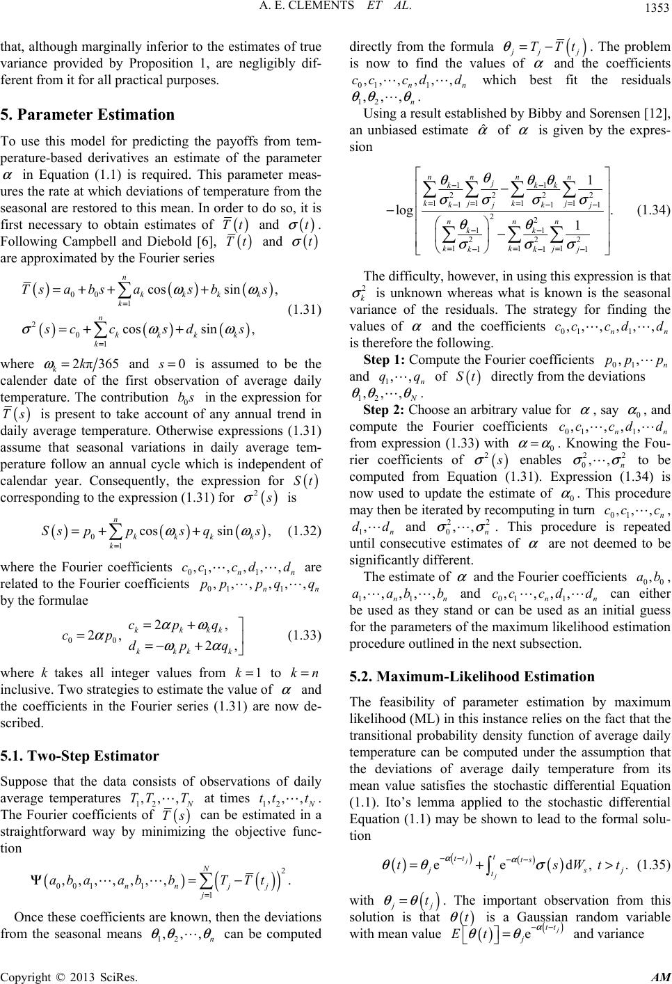

A. E. CLEMENTS ET AL. 1353
that, although marginally inferior to the estimates of true
variance provided by Proposition 1, are negligibly dif-
ferent from it for all practical purposes.
5. Parameter Estimation
To use this model for predicting the payoffs from tem-
perature-based derivatives an estimate of the parameter
α in Equation (1.1) is required. This parameter meas-
ures the rate at which deviations of temperature from the
seasonal are restored to this mean. In order to do so, it is
first necessary to obtain estimates of
()
Tt and
()
t σ .
Following Campbell and Diebold [6],
()
Tt and
()
t σ
are approximated by the Fourier series
() () ()
() () (
00
1
2
0
cossin ,
cos sin
n
kkkk
k
n
kkk
Tsabsas bs
sc csd
ωω
σω
=
=+ ++
=+ +


(1.31)
)
1
,
k
k
s
ω
=
where 2π365
kk
ω = and 0s= is assumed to be the
calender date of the first observation of average daily
temperature. The contribution 0 bs in the expression for
()
Ts is present to take account of any annual trend in
daily average temperature. Otherwise expressions (1.31)
assume that seasonal variations in daily average tem-
perature follow an annual cycle which is independent of
calendar year. Consequently, the expr
corresponding to the expression (1.31) fo
()
2
ession for
r
()
St
s
σ is
() ()()
0
1
cossin ,
n
kkkk
k
Ssppsqs ωω
=
=+ +
 (1.32)
where the Fourier coefficients
related to the Fourier coefficienn
by the formulae
Suppose that the data consists of observations
average temperatures
01 1 ,, ,,, ,
nn
cc cd
ts 01 1 ,,,,,
n
pp pq
d are
,q
00
2,
2, 2,
kkkk
kkk
cpq
cp
dpq
αω
αωα
=+ 
=
=− + (1.33)
where k takes all integer values from 1k= to kn=
inclusive. Two strategies to estimate the value of α and
the coefficients in the Fourier series (1.31) are now de-
scribed.
5.1. Two-Step Estimator
k
of daily
12 ,,,
N
TT T at times 12 ,, ,
N
tt t.
The Fourier coefficients of
(
Tin a
straightforward way by minimizing t
tion
)
s can be estim
he ob
ated
jective func-
()
()
.
j
Tt
()
2
001 1
1
,,,,,,, N
nn j
j
abaabbT
=
Ψ=−


the tions
n beputed
Once these coefficients are known, thendevia
from the seasonal means ca com
directly from the formula
12
,,,
n
θθθ 
()
j
jj
TTt θ =− . The prblem
is now to find the values of
α
and the coefficients
01
,, ,cc
o
which fit the residuals
ybby and Sorensen [12],
1
,, ,
nn
cd d
,,, θθθ .
best
Bi
12 n
Using a result established b
an unbiased estimate ˆ
α
of
α
is given by the expres-
sion
11
2222
1
nn nn
j
kkk
θ
θθθ
σσσ σ
−−
11 1
1
2
2
111
1
.
1
kj j
kjk j
nnn
kkj
j
θθ
σσ σ
== =
−
===
−
1
11
2
11
22
11
k
kk
kk
=
−−
−−
−−
log




−


−

 




−








(1.34)
no
Th f
pute the Fourier coefficients
The difficulty, however, in using this expression is that
2
k
σ is unknown whereas what wn is the seasonal
variance of the residuals. or finding the
values of α and the coefficients 01 1 ,,,,,,
nn
cc cdd
ng.
om
is k
e strategy
is therefore the followi
Step 1: C
an 01 n
d 1,,
n
qq of
()
St directly from the deviations
12
,,,
,,pp p 
N
θθθ .
Step 2: C
compute the
from expr
rier co
hoose an arbitrary vlue for
Fourier coeffi
ession (1.33) with
efficients of
a
cients
αα =
α
01
,,cc
Knowing
, say α , and
0
1
,,,d
the Fo
nn
c d
. u-
0
()
2
s
σ
ation (1
pdate the esti
by reco
22
en
.3
ma
m
ab
1)
te of
puting i
les ,, σσ 
. Exprn
0
α
n t ,
n
cc c,
22
to
. This procedure
01
,,
0
essio
urn
nbe
(1.34) is computed f
now used to
may then be
d
unt
rom Equ
u
iterated
1,n
d and 0,,
n
σσ . This procedure is repeated
il consecutive estimates of α
are not deemed to be
significantly different.
The estimate of
α
and the Fourier coefficients ,ab,
11
,,,,,
nn
aabb and 01 , ,,cc c
be
00
either
1
,
nn
d d can
th
h
m
the
re from its
isfies the
showo the formal solu-
used as they stand or can be used as an initial guess
for the parameters ofe maximum likelihood estimation
procetlined in te next subsection. dure ou
mean va
tio
5.2. Maximum-Likelihood Estimation
The feasibility of parameteration by maximum
likelihood (ML) in this instance relies on the fact that the
transitional probability density function of average daily
temperature can be computed under assumption that
the deviations of average daily temperatu
lue satstochastic differential Equation
(1.1). Ito’s lemma applied to t stochastic differential
Equation (1.1) may be
esti
he
n to lead t
n
()
()
()
()
eed, .
j
j
tt ts
t
j
sj
t
tsWtt
αα
θθ σ
−− −−
=+ >
 (1.35)
with
()
j
j
t θθ =. The important observation from this
solution is that
()
t θ is a Gaussian random variable
with mean value
()
()
e
j
tt
j
θθ = 

Et
α −− and variance

A. E. CLEMENTS ET AL.
1354
()
()
()
22
,e d
tts
ttss
α
χσ
−−
=
()
()
()
2
e,
j
j
jt
tt
j
St St
α −−
=−
(1.36)
where the latter expression for
()
,
j
tt χ t is derived di-
rectly from the definition of
()
St given in Equation
(1.3). Because
() ()
TTt t θ =+ , then the average daily
temperature T is itself Gaussian distributed with mean
value
() ()
()
ej
tt
jj
TtT T
α −−
+− and variance
(
,e
)
()
()
()
2j tt
j
j
t StSt
α −−
=−t χ in which
() () ()
00
1k=
Thus the averageaily temperature
()
Tt has transi-
tional probability
cossin .
n
kkkk
Tta btatbt ωω =+ ++

d
density function
(1.37)
()
()
()
,
e
,, 2π,
Tt
jj
j
fTtTt tt
ψ
χ
−
=, (1.38)
where
() ()
()
()
()
()
2
e
,.
2,
j
tt
j
j
TTt T
Tt tt
α
ψχ
−−
−−
The the sequence
j
T−
=
likelihood of observing12 ,,,
N
TT T
es of average daily temperatures at calendar tim
12
,, ,
N
tt t is therefore
()
()
11
1
,, .
jj jj
j
fT t Tt
++
=
=∏
011 011
1
;,,,,, ;,,,,,,
nnn n
N
aaab bcccdd α
−
 
(1.39)
In practice, the parameters are estimated by minimiz-
ing the negative log-likelihood function
()
()
()
()
(
()
)
1
1
1
12
1
1
2
111
2
11
11
loglog 2πlog e
22
e
1,
2e
jj
jj
jj
Ntt
j
j
j
tt
Njj jj
tt
jjj
NS
TT TT
SS
α
α
α
+
+
+
−−−
+
=
−−
−++
−−
=+
−
−= +−
−−−
+
−


S
(1.40)
where the notation
()
j
j
SSt= has been used. The op-
timal values for the param of this model are taken to
be those which mession (1.39). Although
model (1.1) is s of the intrinsic function
, from a purelyoint of view it is e
treat the Fourier coefficients as the parameters
The task is now to provide a means of gauging the effi-
cacy of the analytical expressions for the mean and vari-
ance of CN given derived previously in terms of the the
expected payoffs to options contracts. Payoffs based on
the analytical results of the paper are compared to h
torical pricing as outlined in [4,5]. The metric for co
parison is taken to be the mean “profit” of a 90-day call
option contract. Profit is defined from the point of view
of the buyer of the call option as the difference be
of the contract and the
maximum and minimum
s for cumulative CDDs are re-
ble 3. There are two observations of note
Table 3. First, the distribution of cumulative
eters
inimize expr
specified in term
technical p
of
()
t σ
to be
asier to
()
St
determined by the ML procedure.
6. Empirical Illustration
is-
m-
tween
the actual tick value expected tick
value or “price” of the option. Of course, this is not
meant to represent a true price for the option, as this no-
tional pricing strategy takes no account of discounting or
overhead expenses. But of course, any pricing scheme
will stand or fall by its ability to estimate the expected
tick value accurately.
6.1. Data
The data set comprises daily
temperature records in degrees Celsius for Brisbane (1/1/
1887-31/8/2007), Melbourne (1/1/1856-31/8/2007), Perth
(1/1/1897-31/8/2007) and Sydney (1/1/1859-31/8/2007).
These locations were chosen primarily because they had
accurate temperature records of over 100 years duration
measured at comparable weather stations4.
Figure 1 shows the long-term expected values (upper
panel) and standard deviations (lower panel) of daily
temperatures for each day of the year. The figure shows
that the behaviour of the mean and standard deviation is
amenable to modelling by a low-order Fourier series ap-
proximation. In this exercise the order of the series is
taken to be 3. The Fourier approximation is applied only
over the period over which the option is to be written,
namely, 1 January to 31 March, inclusive.
Descriptive statistic
ported in Ta
arising from
CDDs for Melbourne is skewed to the right as evidenced
by a mean which is significantly larger than the median.
Second, Perth is notable for the diffuse nature of the dis-
tribution of cumulative CDDs, recording a standard de-
viation significantly larger than those of the other cities.
The distributions of cumulative CDDs for each city is
illustrated in Figure 2 which plots both the distribution
of historical cumulative CDDs (shaded region) and the
predicted distributions for 1950 (dashed line) and 2007
(solid line) generated by closed-form approximations to
the distributions of CDDs derived in the paper. To the
uniformed eye, the distribution of historical cumulative
CDDs may appear well behaved and taken as reasonable
evidence in favour of using historical records to price
temperature-based derivatives. When compared to the
4All the raw data were supplied by Climate Information Services, Na-
tional Climate Centre, Australian Bureau of Meteorology. The con-
struction of the temperature record for each city is discussed in Appen-
dix 3.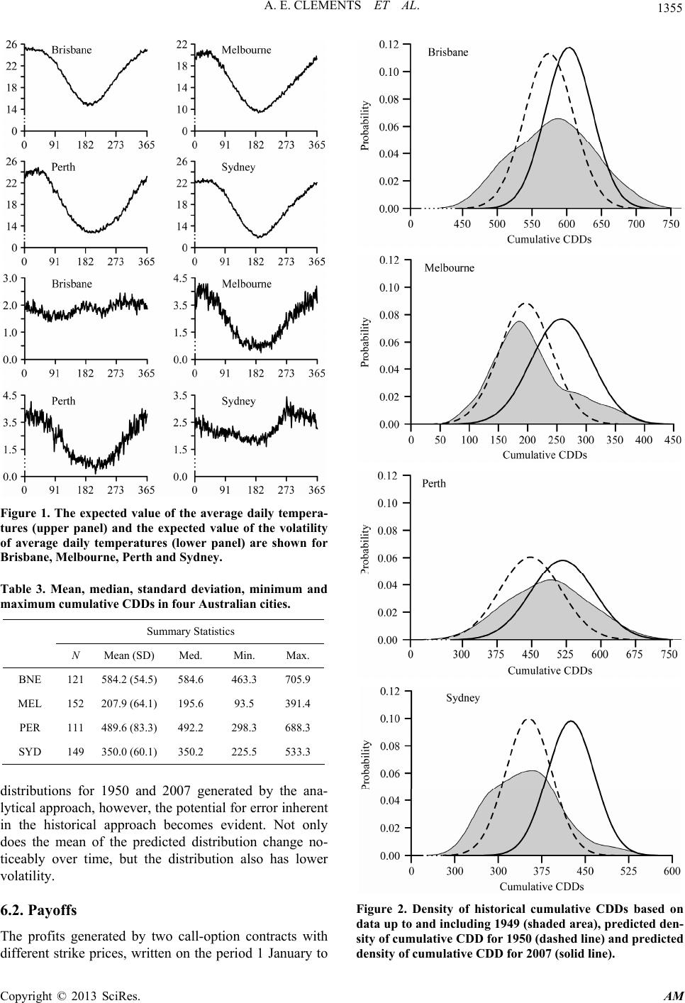

A. E. CLEMENTS ET AL. 1355
Figure 1. The expected value of the average daily tempera-
tures (upper panel) and the expected value of the volatility
of average daily temperatures (lower panel) are shown for
Brisbane, Melbourne, Perth and Sydney.
Table 3. Mean, median, standard deviation, minimum and
maximum cumulative CDDs in four Australian cities.
Summary Statistics
N Mean (SD) Med. Min. Max.
BNE 121 584.2 (54.5) 584.6 463.3 705.9
MEL 152 207.9 (64.1) 195.6 93.5 391.4
PER 111 489.6 (83.3) 492.2 298.3 688.3
SYD 149 350.0 (60.1) 350.2 225.5 533.3
distributions for 1950 and 2007 generated by the ana-
lytical approach, however, the potential for error inheren
with
different strike prices, written on the period 1 January to
t
in the historical approach becomes evident. Not only
does the mean of the predicted distribution change no-
ticeably over time, but the distribution also has lower
volatility.
6.2. Payoffs
The profits generated by two call-option contracts
Figure 2. Density of historical cumulative CDDs based on
data up to and including 1949 (shaded area), predicted den-
sity of cumulative CDD for 1950 (dashed line) and predicted
density of cumulative CDD for 2007 (solid line).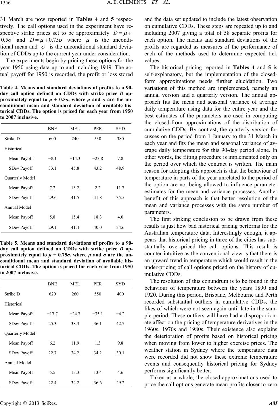

A. E. CLEMENTS ET AL.
1356
31 March are now reported in Tables 4 and 5 respec-
tively. The call options used in the experiment have re-
spective strike prices set to be approximately D
μ
=+
0.5 σ and 0.75D
μ
σ =+ where
μ
e
tion of CDDs up to the current year under consideration.
The experiments begin by pricing these options for the
year 1950 using data up to and including 1949. The ac-
tual payoff for 1950 is recorded, the profit or loss stored
Table 4. Means and standard deviations of profits to a 90-
day call option defined on CDDs with strike price D ap
proximately equal to μ + 0.5σ, where μ and σ are the un
conditional mean and standard deviation of available his-
torical CDDs. The option is priced for each year from 1950
to 2007 inclusive.
BNE MEL PER SYD
is the uncondi-
devia-tional man and
σ
is the unconditional standard
andt updato include the latest observation
on cumese st reed up to and
incl givitotal8 see proor
ehe means and standard deations he
prorded easu thorma of
each ethodsd to ine expected
valu
The historical pricing reported in Tables 4 and 5 is
using data for the entire year and the
best estimates of thee us cong
the cl-from apprations of thestributio of
ce CDDs. Bntrastquar versfo-
cthe period f 1 Janary to t 31 Mah in
eacits thn asoniancv-
erage perature for this-day od alonIn
other words, the fitting procedure is impnted on
the period over which the contract is written. The main
reason for adopting this approach is that the behaviour of
temparts e yeaelatedthe pe of
the not ballowo inflpater
estimhe mean and variance processes. Another
benefit of this approach is thabetter resolution of the
measseshe num of
par
Theking c be d from
icing of call options priced on of-
m
-
-
Strike D 600 240 530 380
Historical
Mean Payoff −8.1 −14.3 −23.8 7.8
SDev Payoff 33.1 45.8 43.2 48.9
Quarterly Model
Mean Payoff 7.2 13.2 2.2 11.7
SDev Payoff 29.6 41.5 41.8 35.5
Annual Model
Mean Payoff 5.8 15.4 18.3 4.0
SDev Payoff 29.1 41.4 40.0 34.6
Table 5. Means and standard deviations of profits to a 90-
day call option defined on CDDs with strike price D ap-
proximately equal to μ + 0.75σ, where μ and σ are the un-
conditional mean and standard deviation of available his-
torical CDDs. The option is priced for each year from 1950
to 2007 inclusive.
BNE MEL PER SYD
Strike D 620 260 550 400
Historical
Mean Payoff −17.7 −24.7 −35.1 −4.2
SDev Payoff
Model
off 6.11.9 1.9.
Annual
5.3 13.4 4.
SDev Payoff 22.4 34.2 36.6 29.2
25.3 38.3 36.1 42.7
Quarterly
Mean Pay2 3 8
SDev Payoff 22.7 34.2 34.2 30.1
Model
Mean Payoff 5 13.6
the data seted
ulative CDDs
uding 2007
. Th
ng a
eps are
of 5
peat
paratfits f
ach option. Tviof t
fits are rega
of the m
as m
use
res of
determ
e perfnce
tick
es.
self-explanatory, but the implementation of the closed-
form approximations needs further elucidation. Two
variations of this method are implemented, namely an
annual version and a quarterly version. The annual ap-
proach fits the mean and seasonal variance of average
daily temperature
e param ters ared inmputi
osed
umulativ
oxim
y co , the
di
terly
n
ion
usses on romuherc
h year and f
daily tem
e meand sea
90
al var
peri
e of a
e.
lemeonly
perature in of thr unr to riod
option are eing ed tuence rame
ates for t
t
n and variance proce with tsameber
ameters.
first strionclusion torawn these
results is just how bad historical pricing performs for the
Australian temperature data. Interestingly enough, it ap-
pears that historical pricing in three of the cities has sub-
stantially over-priced the call options. This result is
counter-intuitive as the conventional view is that there is
an upward trend in temperature which would result in the
under-pr the history cu
ulative CDDs.
The resolution of this conundrum is to be found in the
behaviour of temperature between the years 1890 and
1920. During this period, Brisbane, Melbourne and Perth
recorded substantial outliers in cumulative CDDs, the
likes of which were not seen again until late in the sam-
ple period. These outliers will have had a disproportion-
ate affect on the pricing of temperature derivatives in the
1960s, 1970s and 1980s. Their existence also explains
the deterioration of profits based on historical pricing
when moving from lower to higher exercise prices. The
weather station in Sydney where the temperature data
were recorded did not show these extreme temperature
events and consequently historical pricing for Sydney
performs significantly better.
Taken as a whole, the closed-approximations used to
price the call options generate mean profits closer to zero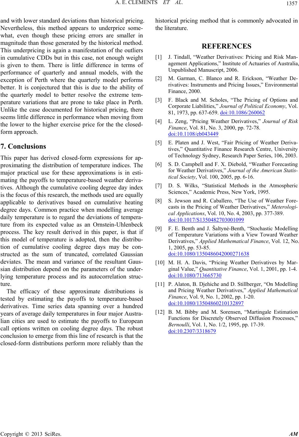

A. E. CLEMENTS ET AL.
1357
icing is again a manifestation of the outliers
in
ence in performance when moving from
th
and with lower standard deviations than historical pricing.
Nevertheless, this method appears to underprice some-
what, even though these pricing errors are smaller in
magnitude than those generated by the historical method.
This underpr
cumulative CDDs but in this case, not enough weight
is given to them. There is little difference in terms of
performance of quarterly and annual models, with the
exception of Perth where the quarterly model performs
better. It is conjectured that this is due to the ability of
the quarterly model to better resolve the extreme tem-
perature variations that are prone to take place in Perth.
Unlike the case documented for historical pricing, there
seems little differ
e lower to the higher exercise price for the the closed-
form approach.
7. Conclusions
This paper has derived closed-form expressions for ap-
proximating the distribution of temperature indices. The
major practical use for these approximations is in esti-
mating the payoffs to temperature-based weather deriva-
tives. Although the cumulative cooling degree day index
is the focus of this research, the methods used are equally
applicable to derivatives based on cumulative heating
degree days. Common practice when modelling average
daily temperature is to regard the deviations of tempera-
ture from its expected value as an Ornstein-Uhlenbeck
process. The key result derived in this paper, is that if
this model of temperature is adopted, then the distribu-
tion of cumulative cooling degree days may be con-
structed as the sum of truncated, correlated Gaussian
deviates. The mean and variance of the resultant Gaus-
sian distribution depend on the parameters of the under-
lying temperature process and its autocorrelation struc-
ture.
The efficacy of these approximate distributions is
tested by estimating the payoffs to temperature-based
derivatives. Time series data spanning over a hundred
years of average daily temperatures in four major Austra-
lian cities are used to estimate the payoffs to European
call options written on cooling degree days. The robust
conclusion to emerge from this line of research is that the
closed-form distributions perform more reliably than the
historical pricing method that is commonly advocated in
the literature.
REFERENCES
[1] J. Tindall, “Weather Derivatives: Pricing and Risk Man-
agement Applications,” Institute of Actuaries of Australia,
Unpublished Manuscript, 2006.
[2] M. Garman, C. Blanco and R. Erickson, “Weather De-
rivatives: Instruments and Pricing Issues,” Environmental
Finance, 2000.
[3] F. Black and M. Scholes, “The Pricing of Options and
Corporate Liabilities,” Journal of Political Economy, Vol.
81, 1973, pp. 637-659. doi:10.1086/260062
[4] L. Zeng, “Pricing Weather Derivatives,” Journal of Risk
Finance, Vol. 81, No. 3, 2000, pp. 72-78.
doi:10.1108/eb043449
[5] E. Platen and J. West, “Fair Pricing of Weather Deriva-
tives,” Quantitative Finance Research Centre, University
of Technology Sydney, Research Paper Series, 106, 2003.
[6] S. D. Campbell and F. X. Diebold, “Weather Forecasting
for Weather Derivatives,” Journal of the American Statis-
tical Society, Vol. 100, 2005, pp. 6-16.
[7] D. S. Wilks, “Statistical Methods in the Atmospheric
Sciences,” Academic Press, New York, 1995.
[8] S. Jewson and of Weather Fore-
casts in the Pritives,” Meterologi-
R. Caballero, “The Use
cing of Weather Deriva
cal Applications, Vol. 10, No. 4, 2003, pp. 377-389.
doi:10.1017/S1350482703001099
[9] F. E. Benth and J. Šaltynė-Benth, “Stochastic Modelling
of Temperature Variations with a View Toward Weather
Derivatives,” Applied Mathematical Finance, Vol. 12, No.
1, 2005, pp. 53-85.
doi:10.1080/1350486042000271638
[10] M. H. A. Davis, “Pricing Weather Derivatives by Mar-
ginal Value,” Quantitative Finance, Vol. 1, 2001, pp. 1-4.
doi:10.1080/713665730
[11] P. Alaton, B. Djehiche and D. Stillberger, “
and Pricing Weather De
On Modelling
rivatives,” Applied Mathematical
Finance, Vol. 9, No. 1, 2002, pp. 1-20.
doi:10.1080/13504860210132897
[12] B. M. Bibby and M. Sorensen, “Martingale Estimation
Functions for Discretely Observed Diffusion Processes,”
Bernoulli, Vol. 1, No. 1/2, 1995, pp. 17-39.
doi:10.2307/3318679

A. E. CLEMENTS ET AL.
1358
Appendix 1
Proof of Result (1.15)
It has been shown in Equation (1.13) that
[]
()
2
k
z
()
The manipulation of this integral uses the fact that the
Gaussian probability density function enjoys the property
. Thus
It is now straightforward algebra to verify the asser-
tion in Equation (1.14), namely that
() ()
2
Var d
.
kk k
kk kk
Szzzz
Sz zz
φ
φ
−∞
=−

−Φ+



() ()
zzz φφ
′
=−
() ()
()
()
()( ) ()
() () () ()
()
() ()
2
22
2
2
2
d
2d
2d
2d
1.
k
k
k
k k
z
kk
z
kk k
z
kk kkk
z z
kk kkkk
kkkkk k
Szzzz
Szzzzzz
SzzSzzz z
SzzSzzzSz z
SzzSz z
φ
φ
φ
φφ
φ
−∞
−∞
−∞
−∞ −∞
−
=−+
′
=Φ+ −
 =Φ+−+

=+Φ+




[
]
Var k  has value
where the calculation has noted that is an even-
valued function of z and that .
Appendix 2
Proof of Result (1.19)
The calculation of
() ()()
()
() ()
()
,
kk kkkkkk
Sz zzzzzz φφ

Φ− +Φ−−Φ−

()
z φ
(
=Φ −
() )
1zz−Φ
[
]
Cov ,
tts+
 requires I, the value
of the integral
()()( )
,dd
tts
zz
t tsttstst
SSzzzwfzzz w
+
+++
−∞ −∞−−
  (1.41)
in which
()
,
ts t
f
zz
+
 is the probability density function
2
1e,
2π
ts
ts t
S
SS
ψ
β
−
+
+−
with
()
22
2
2
2
tst tsts
ts t
Szzw SSSw
SS
β
ψβ
++
+
−+
=−
+
and e
s
α
β
−
=. By re-expressing
ψ
in the form
()
22
2,
2
2
ts t
ts
ts t
SS z
wz
S
SS
β
β
+
+
+

−−


−
() ()()
2d
t
ts t
ts t
t
z S
I
Szzzgzz
SS
φ
β
+−∞
+
=−
− (1.42)
where
()
z φ is the standard normal probabil
nction and
()
ity density
expression (1.41) is re-expressed as the repeated integral
fu
g
z is the integral
()
()
2
2
1
2π
expd .
2
ts
z
ts
t
ts ts
ts t
zw
S
Swz
Sw
SS
β
β
+
+
−∞
+
+
+
−−



−



⋅−

−




(1.43)
Phase I
The evaluation of this integral is achieved by changing
the variable of integration from w to
ξ
using the sub-
stitution
2.
ts t
tstst
SS
wz
SSS
ξβ
β
+
++

=−


−
()
g
z The outcome of this operation is that takes the
simplified form
()
()
()
()
()
2
d
tsz
ts tts
ts
SS
gz z
S
ξ
β
ξξφξξ
+
+
+
−∞
+
−
=−
 (1.44)
where
()
2.
ts t
tsts tsts t
SS
zzz
SSS
ξβ
β
+
++
++

=−


−
It now follows immediately from the definition of
, the cumulative function of the standard normal
tion, and the basic properties of that
()
zΦ
distribu
()
z φ
() ()()
()
2
tsttsts ts
ts
SS
gz S
βφξξ ξ
+
+++
+
−
=+ Φ
(1.45)
in which the dependence of ts
ξ
+
nven
on z has been sup-
pressed for representational coience. Consequently
()
()
()
() ()
2
d.
t
z
tts tt
tsts ts
I
SSSzzz
z
βφ
φξξ ξ
+−∞
+++
=− −
 ×+Φ

 (1.46)
This completes the first phase in the computation of
the value of I using repeated integration.
Phase II
The second phase of calculation continues by dividing
the right hand side of Equation (1.46) into the two inte-
grals

A. E. CLEMENTS ET AL.
1359
()
() ()() ()
()
() ()() ()
2
2
d
d.
t
t
z
ttstttsts ts
z
t tstts
SSSzzz
SSSz zz
βφφξξξ
βφφξξξ
++++
−∞
+ +
−∞
−+Φ
−− +Φ


The function is now replaced by its definition in te inteome rearrangement, I
is expressed as tfour integrals, name
ts ts+ +
he first of thesgrals, and after s
()
ts z
ξ
+
he sum of ly
()
()
()
()
()
() ()
)(
() ()()
2
2
dd
d.
tt
t
zz
tttsttsttst tsts
z
tsttsts ts
IzSSSzzzzSSzz
S zzz
βφξφ ξφ
βφϕξξξ
+++++
−∞ −∞
+ +++
−∞
=−+ Φ
d
t
z
tt tst
z Szzz SS βξ φ
+
−∞


−+Φ−Φ −




(1.47)
The third and fntegrals on the right hand side of this equation are now manipulated using integration by parts.
Manipulation of the third integral gives

ourth i
() () () () () ()
()( ) () ()
2d,
t
z
tts
ts
Sz
z
SS
φφξ
β
+
−∞
+−
(1.48)
2
dd
tt
z z zt
t
ts tsts
t
tts t
S
zzz zzz
S
z
ξφφ ξφφξ
β
φηβ
++ +
−∞ −∞ −∞
+

Φ=−Φ−

=− Φ−

where
ts
S
β
+−
2.
ts tst t
ts
t
S
η
++
+
+
=
s
zS zS β
β
−
−
(1.49)
Manipulation of the fourth integral gives
t
S
()
() ()
()
) () )
()
( ( () ()
() ()()
()
() ()
2
2
d
d
d.
t
tt
t
z
tssts
zz z φφξξ
φ
+++
−∞

=−
t
zz
tsts tsts
ts t
z
t
ttstststs
ts t
zz z
SS
S
zzz
SS
ξ
ϕξξ ξβφξ
β
φφηηη βφξ
β
++++
−∞
−∞ +
+++ +
−∞
+
+Φ

+ Φ−Φ

−
+ Φ−Φ
−


(1.50)
1.50) are notion (1.47
t
S
=−
Results (1.48) and (w incorporated into Equa) to get
() () ()( )
()
() ()
()
()()
2
2
d.
t
z
t
ttsts ttstts
ts t
t tsttts
S
IzS zz
SS
zzS SSz
φξ
β
φ βφφη
+++++
−∞
+
+ +
−∞
=+
−
+−

The final stage of this calculation is note that
d
ts z
φ SS z φ η Φ
(1.51)
t
z
ttst tstts
zz SSS βξ
++ +
++ Φ

to
()
()
()
()
()
2
2
2
2.
tt s tst
ts t
zS z S
SS
β
β
++
+
dexpd
2π2
tt
zz
ts ts t
tsts ts
ts t
tstts
zSS
zzz zz
S
SS
SS
z
S
φ
φξ φβ
β
βφ
++
+ +
−∞ −∞+
+
+
+





=×− −




−

ts+


−
=Φ

To summarize, the repeated integral (1.41) has final value
−


−

()( )()() )(
()
() ()
()
()()
2
d,
ts
zzS SSz
η
βφφη
+
Φ
+−
(1.52)
t
ttst tstt
zz SSS βξ
++ +
−∞
++ Φ

t tsttststst
z
st tsttts
ISSzzz z φχφ
φ
++++
+ +
=Φ+

A. E. CLEMENTS ET AL.
1360
where the constants st+
η
and ts
χ
+
by
and the function
are defined ively
()
ts z
ξ
+ respect
()
2
ts t
tts tst
SS
zS z S
β
β
+
++
−
−
86071) weather station. The location of the office
2
2
,
,
.
ts tst t
ts
ts
ts t
tstst
ts
ts t
zS zS
SS
zS zS
zSS
β
η
χ
β
β
ξ
β
++
+
+
+
++
+
+
−
=
=
−
−
=
−
(1.53)
The construction of the temperature data for the four
Australian cities used in the empirical illustration is now
outlined in detail.
Brisbane: The temperature record contains 44043 ob-
servations starting on the 1/1/1887 and ending on 31/8/
2007. The time series is constructed from data collected
ree weather stations: Brisbane Regional Office
(Station Number 40214) 1/1/1887-31/3/1986; Brisbane
Airport (Station Number 40223) 1/4/1986-14/2/2000);
and again from Brisbane Airport (Station Number 40842)
15/2/2000-31/8/2007.
Melbourne: The temperature record contains 55358
observations starting on 1/1/1856 and ending on 31/8/
2007. The time series is a continuous set of observations
made at the Melbourne Regional Office (Station Number
changed in the early 1980s although the name of station
did not.
Perth: The temperature record contains 40393 obser-
vations starting on 1/1/1897 and ending
The time series is constructed from data collected at two
weather stations: Perth Regional Office (Station Number
Sydney: The temperature record contains 54263 ob-
servations starting on 1/1/1859 and ending on 31/8/2007.
The time series is a continuous set of observations made
at the Sydney Observatory Hill (
weather station.
Instances of single missing values were treated by av-
eraging adjacent records. In a few rare cases where sev-
eral days were missing, the long term average for those
days was inserted. Finally, following Campbell and
Diebold
removed.
Appendix 3
9034) 1/1/1897-2/6/1944; and Perth Airport (Station
Number 9021) 3/6/1944-31/8/2007.
from th
on 31/8/2007.
Station Number 66062)
[6], all occurrences of the 29 February were