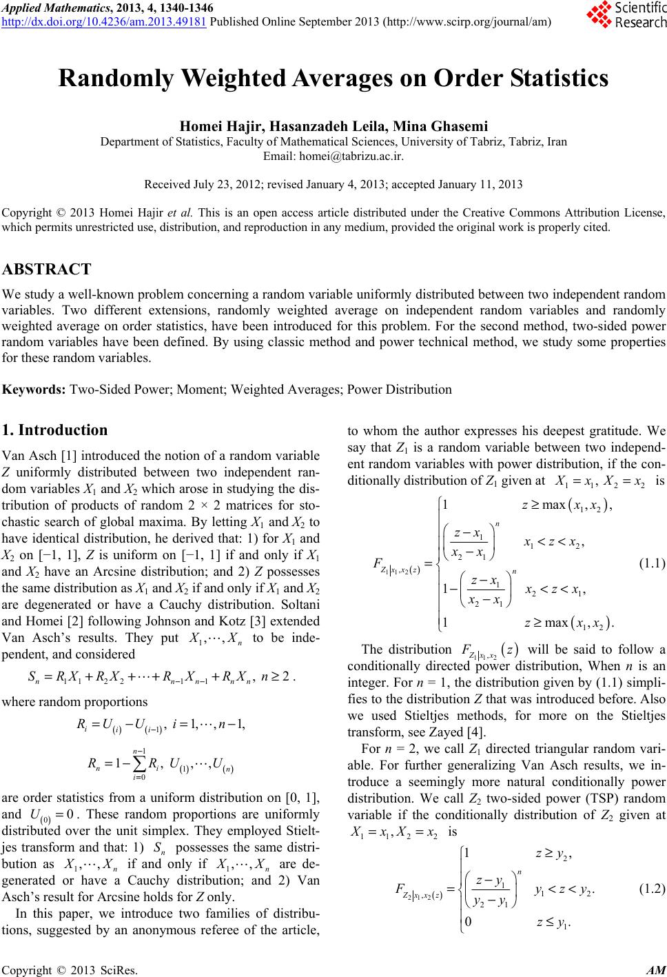
 Applied Mathematics, 2013, 4, 1340-1346 http://dx.doi.org/10.4236/am.2013.49181 Published Online September 2013 (http://www.scirp.org/journal/am) Randomly Weighted Averages on Order Statistics Homei Hajir, Hasanzadeh Leila, Mina Ghasemi Department of Statistics, Faculty of Mathematical Sciences, University of Tabriz, Tabriz, Iran Email: homei@tabrizu.ac.ir. Received July 23, 2012; revised January 4, 2013; accepted January 11, 2013 Copyright © 2013 Homei Hajir et al. This is an open access article distributed under the Creative Commons Attribution License, which permits unrestricted use, distribution, and reproduction in any medium, provided the original work is properly cited. ABSTRACT We study a well-known problem concerning a random variable uniformly distributed between two independent random variables. Two different extensions, randomly weighted average on independent random variables and randomly weighted average on order statistics, have been introduced for this problem. For the second method, two-sided power random variables have been defined. By using classic method and power technical method, we study some properties for these random variables. Keywords: Two-Sided Power; Moment; Weighted Averages; Power Distribution 1. Introduction Van Asch [1] introduced the notion of a random variable Z uniformly distributed between two independent ran- dom variables X1 and X2 which arose in studying the dis- tribution of products of random 2 × 2 matrices for sto- chastic search of global maxima. By letting X1 and X2 to have identical distribution, he derived that: 1) for X1 and X2 on [−1, 1], Z is uniform on [−1, 1] if and only if X1 and X2 have an Arcsine distribution; and 2) Z possesses the same distribution as X1 and X2 if and only if X1 and X2 are degenerated or have a Cauchy distribution. Soltani and Homei [2] following Johnson and Kotz [3] extended Van Asch’s results. They put 1,, n X to be inde- pendent, and considered 112211, 2 nnn SRXRXRX RXn −− =+ +++≥nn U . where random proportions ()( ) 1, 1,,1, iii RU Uin − =−= − ()( ) 1 1 0 1, ,, n ni n i RRU − = =− are order statistics from a uniform distribution on [0, 1], and () 0. These random proportions are uniformly distributed over the unit simplex. They employed Stielt- jes transform and that: 1) n possesses the same distri- bution as 1 0U= S ,, n X if and only if 1,, n X are de- generated or have a Cauchy distribution; and 2) Van Asch’s result for Arcsine holds for Z only. In this paper, we introduce two families of distribu- tions, suggested by an anonymous referee of the article, to whom the author expresses his deepest gratitude. We say that Z1 is a random variable between two independ- ent random variables with power distribution, if the con- ditionally distribution of Z1 given at 112 , 2 xX x== is () () () 11 2 12 1 12 21 , 1 21 21 12 1max , 1, 1max ,, n Zxx zn zxx zx xzx xx Fzx xzx xx zx ≥ −<< − = − −<< − ≥ ,.x (1.1) The distribution () 11 2 ,Zx x z 2 will be said to follow a conditionally directed power distribution, When n is an integer. For n = 1, the distribution given by (1.1) simpli- fies to the distribution Z that was introduced before. Also we used Stieltjes methods, for more on the Stieltjes transform, see Zayed [4]. For n = 2, we call Z1 directed triangular random vari- able. For further generalizing Van Asch results, we in- troduce a seemingly more natural conditionally power distribution. We call Z2 two-sided power (TSP) random variable if the conditionally distribution of Z 2 given at 112 , xX x== is () 21 2 2 1 1 , 21 1 1, . 0. n Zxx z zy zy 2 yzy yy zy ≥ − =< − ≤ < (1.2) C opyright © 2013 SciRes. AM 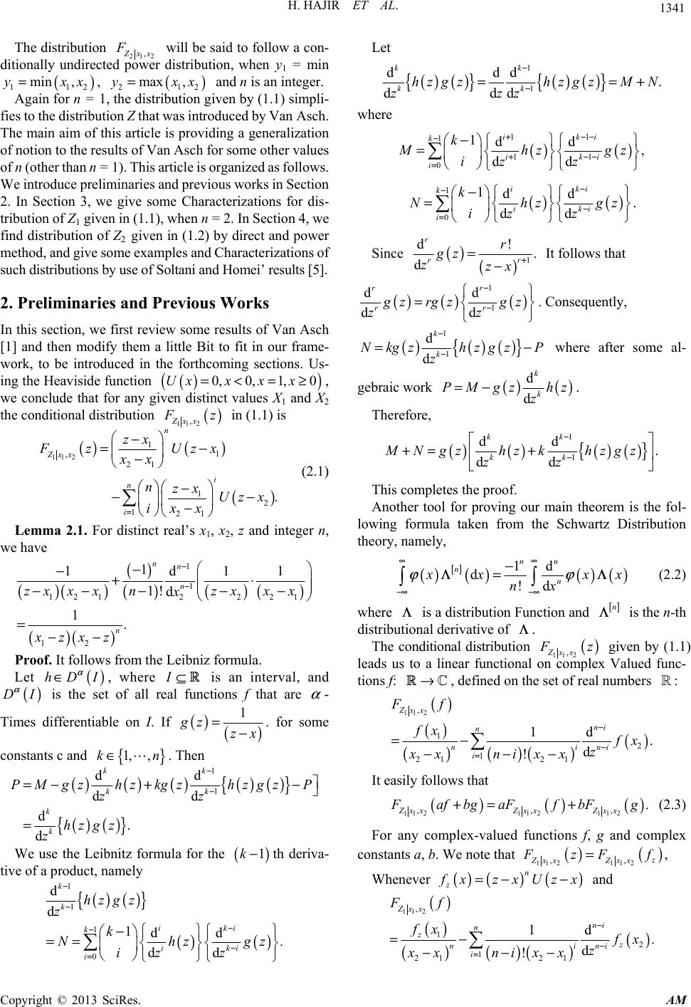 H. HAJIR ET AL. 1341 The distribution 212 , xx will be said to follow a con- ditionally undirected power distribution, when y1 = min F () 11 min,2 xx=, () , 212 max xx= and n is an integer. Again for n = 1, the distribution given by (1.1) simpli- fies to the distribution Z that was introduced by Van Asch. The main aim of this article is providing a generalization of notion to the results of Van Asch for some other values of n (other than n = 1). This article is organized as follows. We introduce preliminaries and previous works in Section 2. In Section 3, we give some Characterizations for dis- tribution of Z1 given in (1.1), when n = 2. In Section 4, we find distribution of Z2 given in (1.2) by direct and power method, and give some examples and Characterizations of such distributions by use of Soltani and Homei’ results [5]. 2. Preliminaries and Previous Works In this section, we first review some results of Van Asch [1] and then modify them a little Bit to fit in our frame- work, to be introduced in the forthcoming sections. Us- ing the Heaviside function , we conclude that for any given distinct values X1 and X2 the conditional distribution () () 0, 0,1, 0Uxxx x=<=≥ () 11 2 ,Zx x z in (1.1) is () () () 11 2 1 1 , 21 1 2 121 . n Zxx i n i zx Fz Uzx xx nzx Uzx ixx = − =− − − −− − (2.1) Lemma 2.1. For distinct real’s x1, x2, z and integer n, we have ()( ) () () ()() ()() 1 1 1212 21 2 12 1 1d1 1! d 1. nn n n zxx xnzxx x x xzxz − − − −+⋅ −− −−− =−− 1 Proof. It follows from the Leibniz formula. Let , where is an interval, and is the set of all real functions f that are - () hDI α ∈ ) II⊆ ( D α α Times differentiable on I. If () () 1 gz zx =−. for some constants c and 1, ,k∈n . Then ()()()() () {} () () {} 1 1 dd dd d. d kk kk k k PMgzhz kgzhzgzP zz hzgz z − − =− +− = We use the Leibnitz formula for the th deriva- tive of a product, namely ( 1k− ) () () {} () () 1 1 1 0 d d 1dd. dd k k iki k iki i hzgz z k Nhz izz − − − − − = − == Let () () {} () () {} 1 1 ddd . d dd kk kk hzgzhzgzM N z zz − − ==+ where () () 11 1 11 0 1dd, dd iki k iki i k hz gz izz +−− − +−− = − = () () 1 0 1dd dd iki k iki i k Nhz izz − − − = −gz = . Since () () 1 d. d r r !r gz zzx + =−r It follows that () ()() 1 1 dd dd rr rr zrgz gz zz − − = . Consequently, ()() () {} 1 1 d d k k N kgzhzgzP z − − =− where after some al- gebraic work () () dk PMgz hz=− dk z. Therefore, () () () () {} 1 1 dd . dd kk kk MNgzhzkhzgz zz − − += + This completes the proof. Another tool for proving our main theorem is the fol- lowing formula taken from the Schwartz Distribution theory, namely, () [] () () () 1d d!d nn n n x nx ϕϕ ∞∞ −∞ −∞ − Λ= Λ xx (2.2) where is a distribution Function and is the n-th distributional derivative of . Λ [] n Λ Λ The conditional distribution () 11 2 ,Zxx z given by (1.1) leads us to a linear functional on complex Valued func- tions f: , defined on the set of real numbers : → () () () ()( )() 11 2 , 1 2 1 21 21 1d . d ! Zxx ni n nin i Ff fx i x z xx nixx − − = =− −−− It easily follows that () () () 11 211 2112 ,, . ZxxZxx Zxx, af bgaFfbFg+= + (2.3) For any complex-valued functions f, g and complex constants a, b. We note that () () 11 211 2 ,, , z Zxx Zxx zF f= Whenever ()()( n z ) xzxUzx=− − and () gz () () ()( )() 11 2 , 1 2 1 21 21 1d . d ! Zxx ni n zz nini i fx Ff x z xx nixx − − = =− −−− Copyright © 2013 SciRes. AM 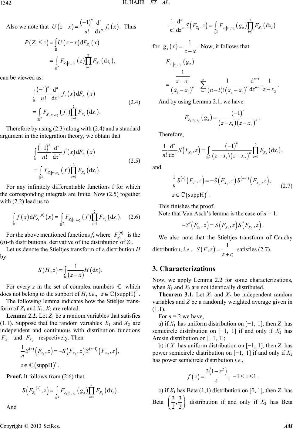 H. HAJIR ET AL. 1342 Also we note that () () () 1d. !d nn z n Uz xfx n − −= Thus ()()() () () 1 11 2 2 1 2 , 1 d d, i Z Xi Zxx i PZzUz xFx zFx = ≤= − = ∏ can be viewed as: () () () () () 1 11 2 2 2 , 1 1dd !d d. i nn zZ n Xi Zxx i xFx nx fFx = − ∏ = (2.4) Therefore by using (2.3) along with (2.4) and a standard argument in the integration theory, we obtain that () () () () () 1 112 2 2 , 1 1dd !d d. i nn Z n Xi Zxx i xFx nx fFx = − = ∏ (2.5) For any infinitely differentiable functions f for which the corresponding integrals are finite. Now (2.5) together with (2.2) lead us to () () () () () 111 2 2 2 , 1 d i nd. Xi Zxx i xFxFfF x = =∏ (2.6) For the above mentioned functions f, where 1 () n is the (n)-th distributional derivative of the distribution of Z1. Let us denote the Stieltjes transform of a distribution H by () () () 1 ,d. SHzH x zx =− For every z in the set of complex numbers which does not belong to the support of H, i.e., . () suppHc z∈ The following lemma indicates how the Stieljes trans- form of Z1 and X1, X2 are related. Lemma 2.2. Let Z1 be a random variables that satisfies (1.1). Suppose that the random variables X1 and X2 are independent and continuous with distribution functions 1 X and 2 X respectively. Then () ()() () () () 11 1 1,, suppH . nn ZXX c SFz SFzSFz n z − =− ∈ 2 ,, Proof. It follows from (2.6) that () () () () 111 2 2 2 , 1 , i nd zX Zxx i SFzFgF x = =∏ i . And () () () 111 2 2 2 , 1 1d ,d !d i n zX Zx x ni SF zFgFx nz = =∏ i for () 1 z gx zx =−. Now, it follows that () ()()() 11 2 , 1 12 21 21 1 1d1 . d ! z Zxx ni n ni i Fg zx zzx xx nixx − − = − =− − −−− ni And by using Lemma 2.1, we have () () ()() 11 2 , 12 1. n z Zxx n Fg zxzx − =−− Therefore, () () ()() () 1 2 2 1 12 1 1d ,d !di n n ZX nn i SF zFx nzzx zx= − =−− ∏ , i and () ()() () () () 11 1 1,, suppH . nn ZXX c SFz SFzSFz n z − =− ∈ 2 ,, ) 2 , (2.7) This finishes the proof. Note that Van Asch’s lemma is the case of n = 1: ()()( 11 ,, ZXX SF zSFzSFz ′ −= . We also note that the Stieltjes transform of Cauchy distribution, i.e., () 1 ,SFz zc =+ satisfies (2.7). 3. Characterizations Now, we apply Lemma 2.2 for some characterizations, when X1 and X2 are not identically distributed. Theorem 3.1. Let X1 and X2 be independent random variables and Z be a randomly weighted average given in (1.1). For n = 2 we have, a) if X1 has uniform distribution on [−1, 1], then Z1 has semicircle distribution on [−1, 1] if and only if X2 has Arcsin distribution on [−1, 1]; b) if X1 has uniform distribution on [−1, 1], then Z1 has power semicircle distribution on [−1, 1] if and only if X2 has power semicircle distribution i.e., () () 2 31 , 11 4 z zz − =−≤≤ . c) if X1 has Beta (1,1) distribution on [0, 1], then Z1 has Beta 33 , 22 distribution if and only if X2 has Beta Copyright © 2013 SciRes. AM 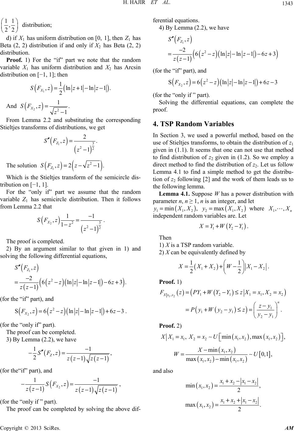 H. HAJIR ET AL. 1343 11 , 22 distribution; d) if X1 has uniform distribution on [0, 1], then Z1 has Beta (2, 2) distribution if and only if X2 has Beta (2, 2) distribution. Proof. 1) For the “if” part we note that the random variable X1 has uniform distribution and X2 has Arcsin distribution on [−1, 1]; then () () 1 1 ,ln1ln 2 X SF zzz=+−− 1. And () 22 1 ,. 1 X SF zz = − From Lemma 2.2 and substituting the corresponding Stieltjes transforms of distributions, we get () () 13 22 2 ,. 1 Z SFz z ′′ = − The solution () () 1 2 ,2 1. Z SF zzz=−− Which is the Stieltjes transform of the semicircle dis- tribution on [−1, 1]. For the “only if” part we assume that the random variable Z1 has semicircle distribution. Then it follows from Lemma 2.2 that () () 223 22 11 ,11 X SF zzz − = −− . The proof is completed. 2) By an argument similar to that given in 1) and solving the following differential equations, () () () () () 1 2 , 26lnln16 1 Z SFz zz zzz zz ′′ − =−−−− −3.+ (for the “if” part), and () () () 2 2 S,6 lnln16 X3 zzzzzz=− −−+−. (for the “only if” part). The proof can be completed. 3) By Lemma (2.2), we have () ()() 11 ,, 211 Z SFz zz zz − ′′ −= −− (for the“if” part), and () () ()() 2 11 , 111 X SF z zz zz zz − −= −−− , (for the “only if ” part). The proof can be completed by solving the above dif- ferential equations. 4) By Lemma (2.2), we have () () () () () 1 2 , 26lnln16 1 Z SFz zz zzz zz ′′ − =−−−− −3+ (for the “if” part), and () () () 2 2 S,6 lnln16 X3 zzzzzz=− −−+− (for the “only if ” part). Solving the differential equations, can complete the proof. 4. TSP Random Variables In Section 3, we used a powerful method, based on the use of Stieltjes transforms, to obtain the distribution of z1 given in (1.1). It seems that one can not use that method to find distribution of z2 given in (1.2). So we employ a direct method to find the distribution of z2. Let us follow Lemma 4.1 to find a simple method to get the distribu- tion of z2 following [2] and the work of them leads us to the following lemma. Lemma 4.1. Suppose W has a power distribution with parameter n, n ≥ 1, n is an integer, and let 212 =1,, n () 11 min ,yXX=, () ,yX 2 max X where X random variables are. Let independent () 121 YWYY=+−. Then 1) X is a TSP random variable. 2) X can be equivalently defined by () 12 12 11 22 XX WXX =++−− . Proof. 1) ()( ) () () () 12 121 112 , 1 121 21 , . Xx x n 2 zPYWYYzXxXx zy Py Wyyzyy =+ −≤== − =+ −≤= − Proof. 2) () () 11221212 , min,,max,,XXx XxUxxxx== () () () [] 12 12 12 min ,0,1 , max ,min , Xxx WU xx xx − =− and also () 12 12 12 min ,, 2 xxx xx +−− = () 12 12 12 max ,. 2 xxx xx ++− = Copyright © 2013 SciRes. AM 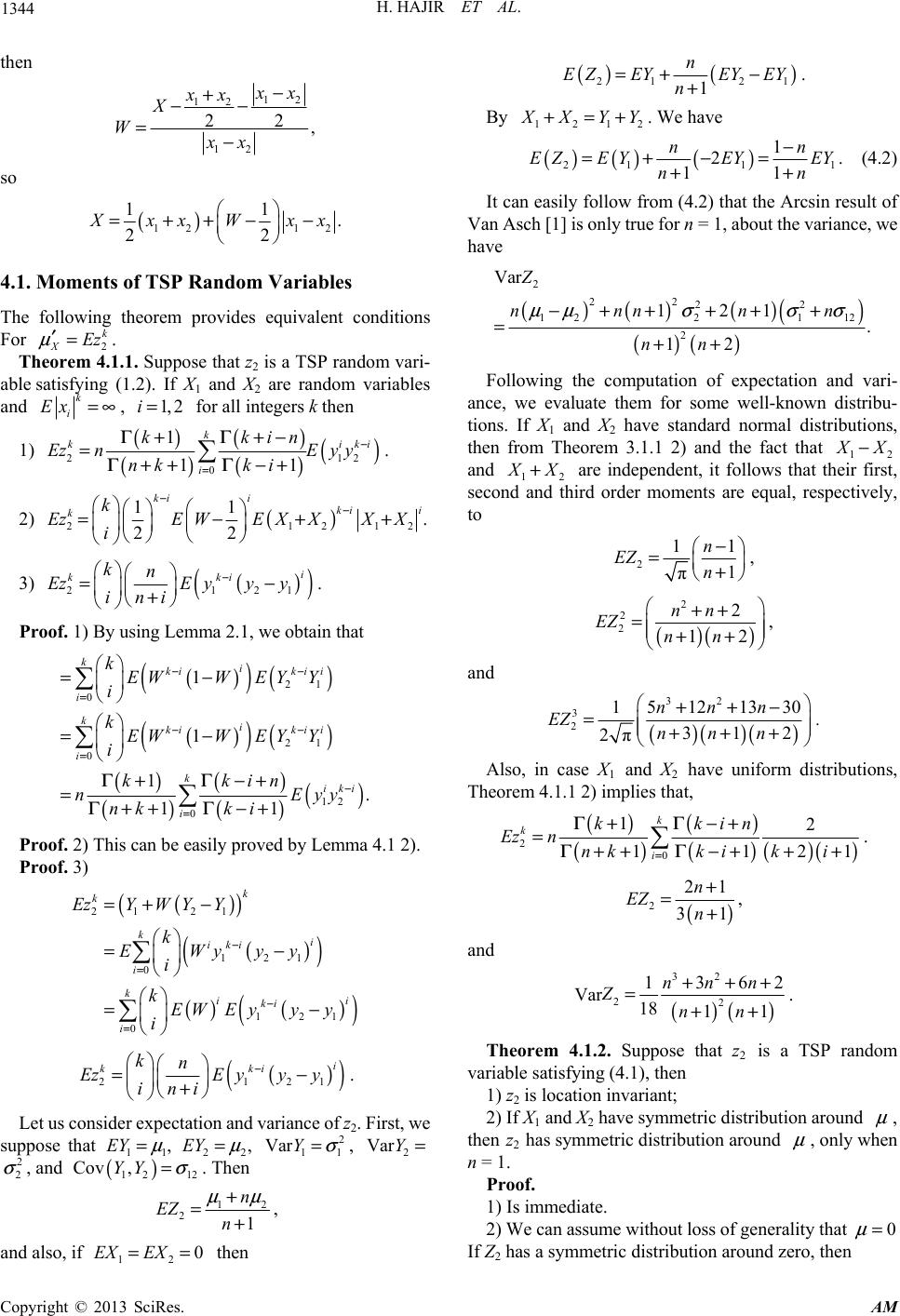 H. HAJIR ET AL. 1344 then 12 12 12 22 , x xx X Wxx − + −− =− so () 12 12 11 . 22 xx Wxx =++−− 4.1. Moments of TSP Random Variables The following theorem provides equivalent conditions For . 2 Theorem 4.1.1. Suppose that z2 is a TSP random vari- ablesatisfying (1.2). If X1 and X2 are random variables and k XEz μ ′= k i Ex =∞, for all integers k then 1, 2i= () 1) () () () () 2 0 1 11 k i Ez nEy y nk ki − = =Γ+ + Γ−+ 12 i ki k kkin−Γ+ Γ+. 2) () 21 11 22 ki iiki kk EzEWEX XX X i − − =−+ 212 + . 3) () () 21 i kki kn EzE yyy ini − =− + 21 . Proof. 1) By using Lemma 2.1, we obtain that () () () () () () () () () () () 21 0 21 0 12 0 1 1 1. 11 ki kiki i i ki kiki i i kiki i kEWWEY Y i kEWWEY Y i kkin n nk ki −− = −− = − = =− =− Γ+ Γ−+ =Γ++ Γ−+ E yy Proof. 2) This can be easily proved by Lemma 4.1 2). Proof. 3) () () () () ()( ) () 21 21 121 0 121 0 k k ki iki i kii ki i EzYW YY k EWyyy i kEWE yyy i − = − = =+ − =− =− () () 21 i kki kn EzE yyy ini − = + 21 −. Let us consider expectation and variance of z2. First, we suppose that 11 EY =, 22 EY = 12 σ , , , and . Then 2 11 VarY σ =2 Y=Var 2 2 σ () 12 ,YY =Cov 12 21 n EZ n + =+, and also, if then 12 0EXEX== () () 21 2 1 n E ZEYEYEY n =+ − +1 . By 1212 XYY+=+. We have () ()() 21 1 1 2 11 nn EZ EYEYEY nn − =+−= ++ 1 . (4.2) It can easily follow from (4.2) that the Arcsin result of Van Asch [1] is only true for n = 1, about the variance, we have ( )()() () ()( ) 2 22 22 1221 12 2 Var 121. 12 Z nnnnn nn μμσσ σ −++++ + =++ Following the computation of expectation and vari- ance, we evaluate them for some well-known distribu- tions. If X1 and X2 have standard normal distributions, then from Theorem 3.1.1 2) and the fact that 12 X− and 12 X+ are independent, it follows that their first, second and third order moments are equal, respectively, to 2 11 1 π n EZ n − = + , ()( ) 2 2 2 2 12 nn EZ nn ++ = ++ , and ()()() 32 3 2 151213 30 312 2π nnn EZ nnn ++− = +++ . Also, in case X1 and X2 have uniform distributions, Theorem 4.1.1 2) implies that, () () () () ()() 2 0 12 112 k k i kkin Eznnkkiki = Γ+Γ−+ =Γ++Γ−++ + 1 . () 2 21 31 n EZ n + =+, and ()() 32 22 136 Var 18 11 nnn Znn +++ =++ 2 . Theorem 4.1.2. Suppose that z2 is a TSP random variable satisfying (4.1), then 1) z2 is location invariant; 2) If X1 and X2 have symmetric distribution around , then z2 has symmetric distribution around , only when n = 1. Proof. 1) Is immediate. 2) We can assume without loss of generality that 0 = If Z2 has a symmetric distribution around zero, then Copyright © 2013 SciRes. AM 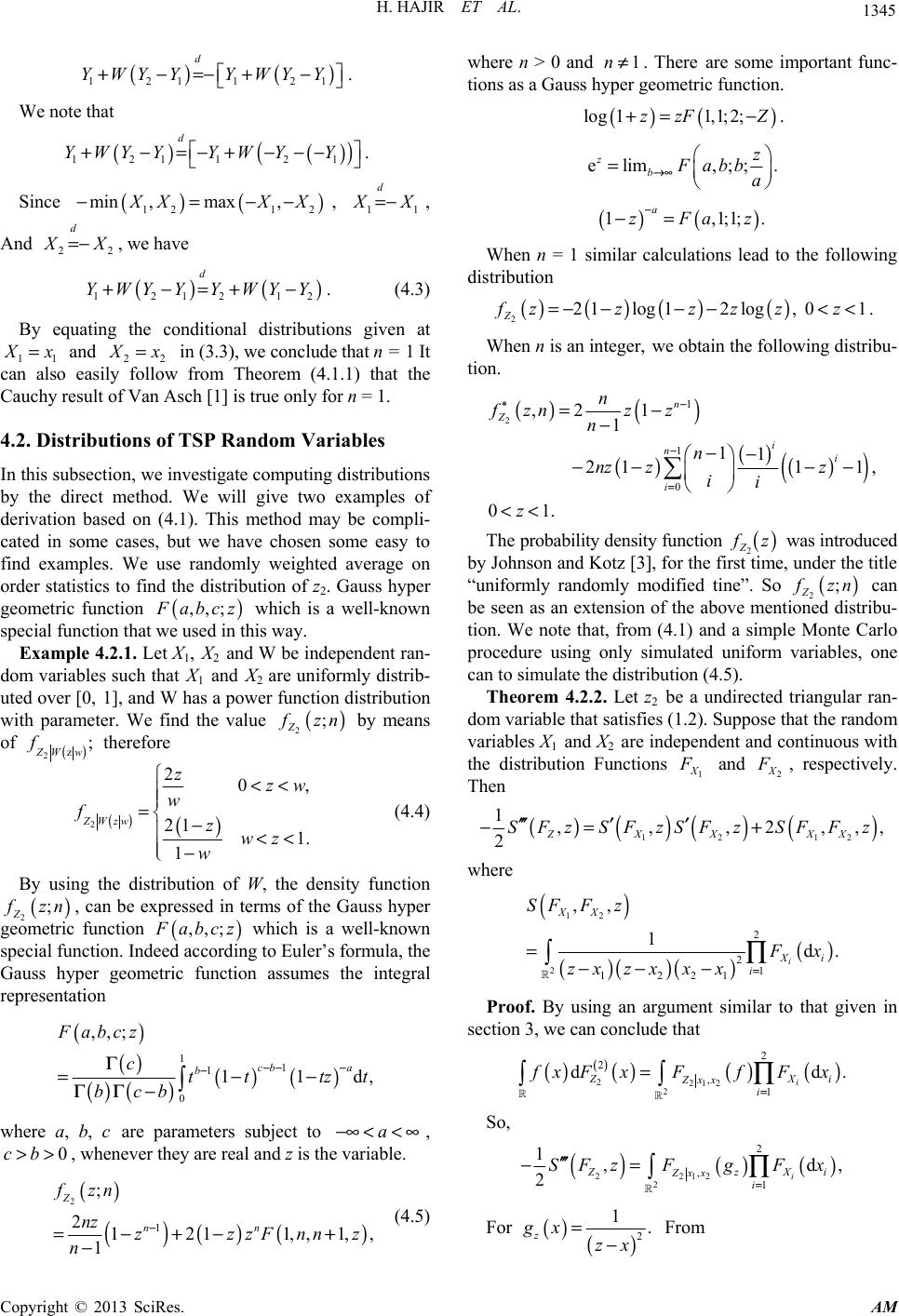 H. HAJIR ET AL. 1345 () ( 121121 d YWYY YWYY+−=−+− ) . We note that () () () 1211 21 d YWYYYWY Y +−=−+−−− . Since ()( 1212 min ,max, ) XX−=−X 11 d −, X=− , And 22 d X=− , we have () ( 12121 d YWYYYWYY+−=+− ) 2 . (4.3) By equating the conditional distributions given at 11 x= and 22 x= in (3.3), we conclude that n = 1 It can also easily follow from Theorem (4.1.1) that the Cauchy result of Van Asch [1] is true only for n = 1. 4.2. Distributions of TSP Random Variables In this subsection, we investigate computing distributions by the direct method. We will give two examples of derivation based on (4.1). This method may be compli- cated in some cases, but we have chosen some easy to find examples. We use randomly weighted average on order statistics to find the distribution of z2. Gauss hyper geometric function ( ,,; ) abcz which is a well-known special function that we used in this way. Example 4.2.1. Let X1, X2 and W be independent ran- dom variables such that X1 and X2 are uniformly distrib- uted over [0, 1], and W has a power function distribution with parameter. We find the value ( 2; ) Z zn by means of () 2z; Ww f therefore () () 2 20, 21 1. 1 ZWzw zzw w fzwz w << =− << − ) (4.4) By using the distribution of W, the density function 2 ( ; Z zn , can be expressed in terms of the Gauss hyper geometric function ( ,,; ) abcz which is a well-known special function. Indeed according to Euler’s formula, the Gauss hyper geometric function assumes the integral representation () () () ()()( ) 11 1 0 ,,; 11 cb a b F abcz ctt tz bcb −− − − Γ =− ΓΓ− d,t − where a, b, c are parameters subject to , , whenever they are real and z is the variable. a−∞ <<∞ 0cb>> () () ()( ) 2 1 ; 2121 1,,1, 1 Z nn fzn nz zzzFnn n − =−+−+ − where n > 0 and . There are some important func- tions as a Gauss hyper geometric function. 1n≠ ,z ) (4.5) () ( log11,1; 2;zzFZ+= −. elim ,;;. zbz Fabb →∞ = a () () 1, 1; 1;. a zFaz − −= When n = 1 similar calculations lead to the following distribution ()( )() 2log12log, 01 Z ( ) 21 zz−zzz=−−−<<z. When n is an integer, we obtain the following distribu- tion. () () () () () () 2 1 1 0 ,2 1 1 11 211 1 01. n Z i ni i n fznzz n n nz zz ii z ∗− − = =− − −− −− −− << , The probability density function 2 Z () z was introduced by Johnson and Kotz [3], for the first time, under the title “uniformly randomly modified tine”. So 2 ( ; Z ) zn can be seen as an extension of the above mentioned distribu- tion. We note that, from (4.1) and a simple Monte Carlo procedure using only simulated uniform variables, one can to simulate the distribution (4.5). Theorem 4.2.2. Let z2 be a undirected triangular ran- dom variable that satisfies (1.2). Suppose that the random variables X1 and X2 are independent and continuous with the distribution Functions 1 X and 2 X , respectively. Then () ()()( 12 12 1,,,2, ZXX XX z SFzSFzSFFz ′ ′ −= + ) ,, 2SF ′′′ where () ()()() () 12 2 2 2 1 1221 ,, 1d. i XX Xi i SF Fz x zx zxxx= =−− − ∏ Proof. By using an argument similar to that given in section 3, we can conclude that () () () () () 221 2 2 2 2 , 1 dd i. Xi Zxx i xF xFfFx = =∏ So, () () () 221 2 2 2 , 1 1,d 2i Zz Zxx i SFzFgF x = ′′′ −= ∏ , Xi For () () 2 1. z gx zx =− From Copyright © 2013 SciRes. AM 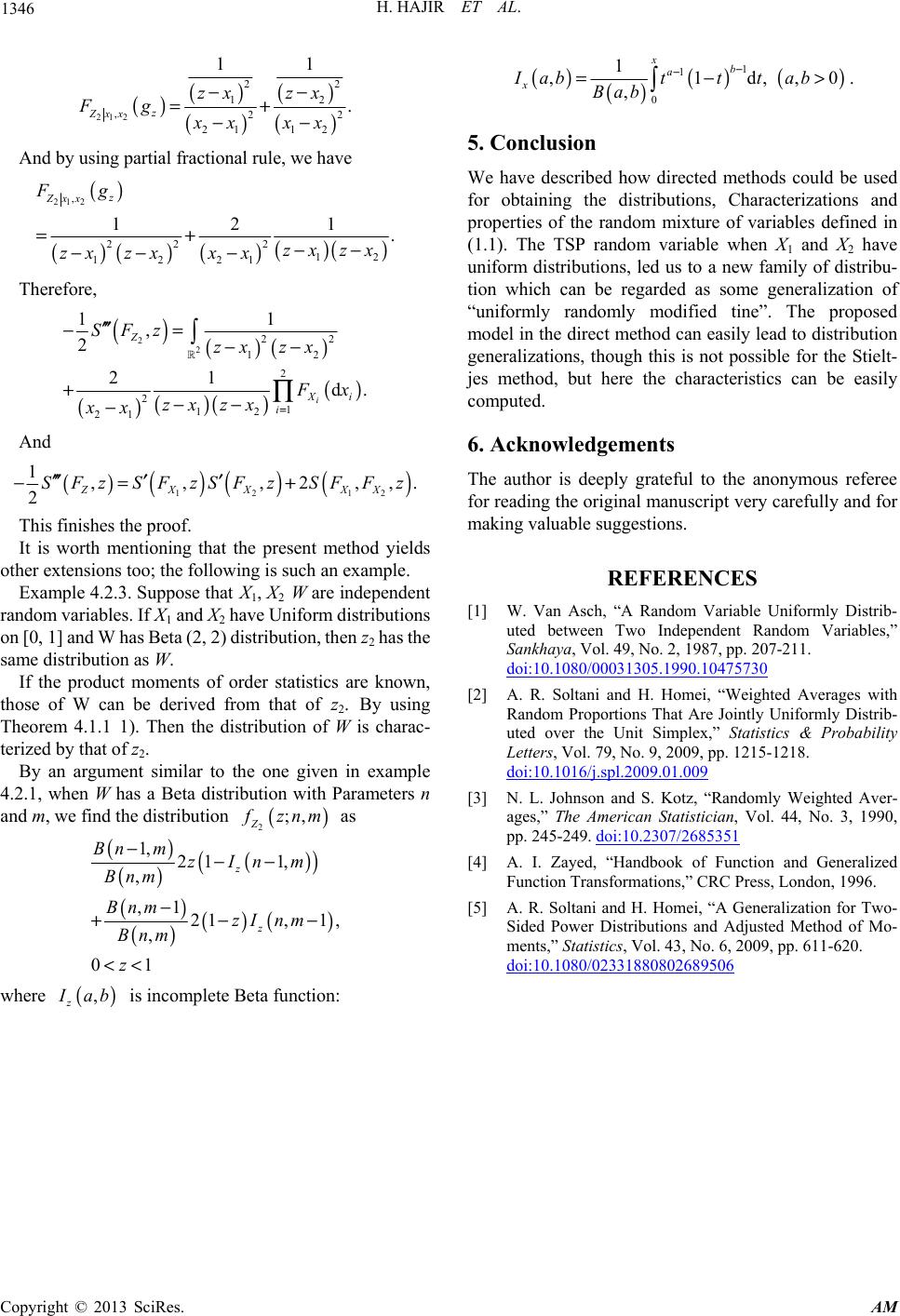 H. HAJIR ET AL. Copyright © 2013 SciRes. AM 1346 ()() () () () 21 2 22 12 ,22 21 12 11 . z Zxx zx zx Fg xx xx −− =+ −− () () () ( 1 1 0 ) 0> 1 ,1d, , , xb a x Iabtttab Bab − − =− . 5. Conclusion And by using partial fractional rule, we have We have described how directed methods could be used for obtaining the distributions, Characterizations and properties of the random mixture of variables defined in (1.1). The TSP random variable when X1 and X2 have uniform distributions, led us to a new family of distribu- tion which can be regarded as some generalization of “uniformly randomly modified tine”. The proposed model in the direct method can easily lead to distribution generalizations, though this is not possible for the Stielt- jes method, but here the characteristics can be easily computed. () ()() () ()() 21 2 , 22 2 12 1221 121 . z Zxx Fg zx zx zxzxx x =+ −− −− − Therefore, () ()() () ()()() 2 2 22 12 2 2 1 12 21 11 , 2 21 d. i Z Xi i SFz zxzx x zx zx xx = ′′′ −= −− +−− − ∏ 6. Acknowledgements And () ()()( 12 12 1,,,2, 2ZXX XX SFz SFzSFzSFFz ′′′′ ′ −=+ ) ,. The author is deeply grateful to the anonymous referee for reading the original manuscript very carefully and for making valuable suggestions. This finishes the proof. It is worth mentioning that the present method yields other extensions too; the following is such an example. REFERENCES Example 4.2.3. Suppose that X1, X2 W are independent random variables. If X1 and X2 have Uniform distributions on [0, 1] and W has Beta (2, 2) distribution, then z2 has the same distribution as W. [1] W. Van Asch, “A Random Variable Uniformly Distrib- uted between Two Independent Random Variables,” Sankhaya, Vol. 49, No. 2, 1987, pp. 207-211. doi:10.1080/00031305.1990.10475730 If the product moments of order statistics are known, those of W can be derived from that of z2. By using Theorem 4.1.1 1). Then the distribution of W is charac- terized by that of z2. [2] A. R. Soltani and H. Homei, “Weighted Averages with Random Proportions That Are Jointly Uniformly Distrib- uted over the Unit Simplex,” Statistics & Probability Letters, Vol. 79, No. 9, 2009, pp. 1215-1218. doi:10.1016/j.spl.2009.01.009 By an argument similar to the one given in example 4.2.1, when W has a Beta distribution with Parameters n and m, we find the distribution () 2;, Z znm as [3] N. L. Johnson and S. Kotz, “Randomly Weighted Aver- ages,” The American Statistician, Vol. 44, No. 3, 1990, pp. 245-249. doi:10.2307/2685351 () () () () () () ()( ) 1, 211, , ,1 21,1, , 01 z z Bnm zInm Bnm Bnm zI nm Bnm z −−− − +− << [4] A. I. Zayed, “Handbook of Function and Generalized Function Transformations,” CRC Press, London, 1996. [5] A. R. Soltani and H. Homei, “A Generalization for Two- Sided Power Distributions and Adjusted Method of Mo- ments,” Statistics, Vol. 43, No. 6, 2009, pp. 611-620. doi:10.1080/02331880802689506 − where ( , z ) ab is incomplete Beta function:
|