Paper Menu >>
Journal Menu >>
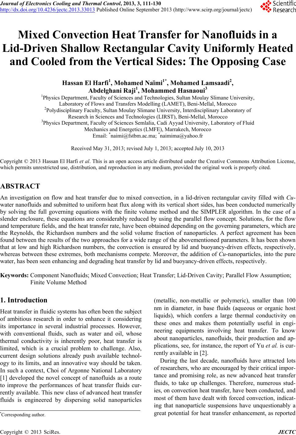 Journal of Electronics Cooling and Thermal Control, 2013, 3, 111-130 http://dx.doi.org/10.4236/jectc.2013.33013 Published Online September 2013 (http://www.scirp.org/journal/jectc) Mixed Convection Heat Transfer for Nanofluids in a Lid-Driven Shallow Rectangular Cavity Uniformly Heated and Cooled from the Vertical Sides: The Opposing Case Hassan El Harfi1, Mohamed Naïmi1*, Mohamed Lamsaadi2, Abdelghani Raji1, Mohammed Hasnaoui3 1Physics Department, Faculty of Sciences and Technologies, Sultan Moulay Slimane University, Laboratory of Flows and Transfers Modelling (LAMET), Beni-Mellal, Morocco 2Polydisciplinary Faculty, Sultan Moulay Slimane University, Interdisciplinary Laboratory of Research in Sciences and Technologies (LIRST), Beni-Mellal, Morocco 3Physics Department, Faculty of Sciences Semlalia, Cadi Ayyad University, Laboratory of Fluid Mechanics and Energetics (LMFE), Marrakech, Morocco Email: *naimi@fstbm.ac.ma; *naimima@yahoo.fr Received May 31, 2013; revised July 1, 2013; accepted July 10, 2013 Copyright © 2013 Hassan El Harfi et al. This is an open access article distributed under the Creative Commons Attribution License, which permits unrestricted use, distribution, and reproduction in any medium, provided the original work is properly cited. ABSTRACT An investigation on flow and heat transfer due to mixed convection, in a lid-driven rectangular cavity filled with Cu- water nanofluids and submitted to uniform heat flux along with its vertical short sides, has been conducted numerically by solving the full governing equations with the finite volume method and the SIMPLER algorithm. In the case of a slender enclosure, these equations are considerably reduced by using the parallel flow concept. Solutions, for the flow and temperature fields, and the heat transfer rate, have been obtained depending on the governing parameters, which are the Reynolds, the Richardson numbers and the solid volume fraction of nanoparticles. A perfect agreement has been found between the results of the two approaches for a wide range of the abovementioned parameters. It has been shown that at low and high Richardson numbers, the convection is ensured by lid and buoyancy-driven effects, respectively, whereas between these extremes, both mechanisms compete. Moreover, the addition of Cu-nanoparticles, into the pure water, has been seen enhancing and degrading heat transfer by lid and buoyancy-driven effects, respectively. Keywords: Component Nanofluids; Mixed Convection; Heat Transfer; Lid-Driven Cavity; Parallel Flow Assumption; Finite Volume Method 1. Introduction Heat transfer in fluidic systems has often been the subject of ambitious research in order to enhance it considering its importance in several industrial processes. However, with conventional fluids, such as water and oil, whose thermal conductivity is inherently poor, heat transfer is limited, which is a crucial problem to challenge. Also, current design solutions already push available technol- ogy to its limits, and an innovative way should be taken. In such a context, Choi of Argonne National Laboratory [1] developed the novel concept of nanofluids as a route to improve the performances of heat transfer fluids cur- rently available. This new class of advanced heat transfer fluids is engineered by dispersing solid nanoparticles (metallic, non-metallic or polymeric), smaller than 100 nm in diameter, in base fluids (aqueous or organic host liquids), which confers a large thermal conductivity on these ones and makes them potentially useful in engi- neering equipments involving heat transfer. To know about nanoparticles, nanofluids, their production and ap- plications, see, for instance, the report of Yu et al. is cur- rently available in [2]. During the last decade, nanofluids have attracted lots of researchers, who are encouraged by their critical impor- tance and promising role, as new advanced heat transfer fluids, to take up challenges. Therefore, numerous stud- ies, on convection heat transfer, have been conducted, and most of them have dealt with forced convection, indicat- ing that nanoparticle suspensions have unquestionably a great potential for heat transfer enhancement, as reported *Corresponding author. C opyright © 2013 SciRes. JECTC 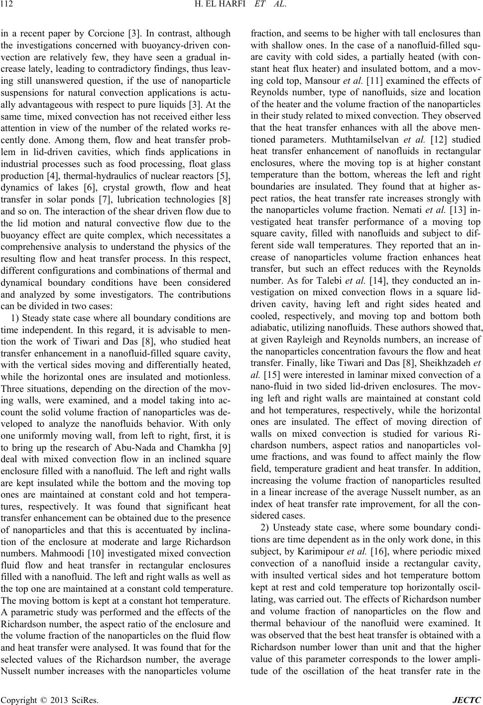 H. EL HARFI ET AL. 112 in a recent paper by Corcione [3]. In contrast, although the investigations concerned with buoyancy-driven con- vection are relatively few, they have seen a gradual in- crease lately, leading to contradictory findings, thus leav- ing still unanswered question, if the use of nanoparticle suspensions for natural convection applications is actu- ally advantageous with respect to pure liquids [3]. At the same time, mixed convection has not received either less attention in view of the number of the related works re- cently done. Among them, flow and heat transfer prob- lem in lid-driven cavities, which finds applications in industrial processes such as food processing, float glass production [4], thermal-hydraulics of nuclear reactors [5], dynamics of lakes [6], crystal growth, flow and heat transfer in solar ponds [7], lubrication technologies [8] and so on. The interaction of the shear driven flow due to the lid motion and natural convective flow due to the buoyancy effect are quite complex, which necessitates a comprehensive analysis to understand the physics of the resulting flow and heat transfer process. In this respect, different configurations and combinations of thermal and dynamical boundary conditions have been considered and analyzed by some investigators. The contributions can be divided in two cases: 1) Steady state case where all boundary conditions are time independent. In this regard, it is advisable to men- tion the work of Tiwari and Das [8], who studied heat transfer enhancement in a nanofluid-filled square cavity, with the vertical sides moving and differentially heated, while the horizontal ones are insulated and motionless. Three situations, depending on the direction of the mov- ing walls, were examined, and a model taking into ac- count the solid volume fraction of nanoparticles was de- veloped to analyze the nanofluids behavior. With only one uniformly moving wall, from left to right, first, it is to bring up the research of Abu-Nada and Chamkha [9] deal with mixed convection flow in an inclined square enclosure filled with a nanofluid. The left and right walls are kept insulated while the bottom and the moving top ones are maintained at constant cold and hot tempera- tures, respectively. It was found that significant heat transfer enhancement can be obtained due to the presence of nanoparticles and that this is accentuated by inclina- tion of the enclosure at moderate and large Richardson numbers. Mahmoodi [10] investigated mixed convection fluid flow and heat transfer in rectangular enclosures filled with a nanofluid. The left and right walls as well as the top one are maintained at a constant cold temperature. The moving bottom is kept at a constant hot temperature. A parametric study was performed and the effects of the Richardson number, the aspect ratio of the enclosure and the volume fraction of the nanoparticles on the fluid flow and heat transfer were analysed. It was found that for the selected values of the Richardson number, the average Nusselt number increases with the nanoparticles volume fraction, and seems to be higher with tall enclosures than with shallow ones. In the case of a nanofluid-filled squ- are cavity with cold sides, a partially heated (with con- stant heat flux heater) and insulated bottom, and a mov- ing cold top, Mansour et al. [11] examined the effects of Reynolds number, type of nanofluids, size and location of the heater and the volume fraction of the nanoparticles in their study related to mixed convection. They observed that the heat transfer enhances with all the above men- tioned parameters. Muthtamilselvan et al. [12] studied heat transfer enhancement of nanofluids in rectangular enclosures, where the moving top is at higher constant temperature than the bottom, whereas the left and right boundaries are insulated. They found that at higher as- pect ratios, the heat transfer rate increases strongly with the nanoparticles volume fraction. Nemati et al. [13] in- vestigated heat transfer performance of a moving top square cavity, filled with nanofluids and subject to dif- ferent side wall temperatures. They reported that an in- crease of nanoparticles volume fraction enhances heat transfer, but such an effect reduces with the Reynolds number. As for Talebi et al. [14], they conducted an in- vestigation on mixed convection flows in a square lid- driven cavity, having left and right sides heated and cooled, respectively, and moving top and bottom both adiabatic, utilizing nanofluids. These authors showed that, at given Rayleigh and Reynolds numbers, an increase of the nanoparticles concentration favours the flow and heat transfer. Finally, like Tiwari and Das [8], Sheikhzadeh et al. [15] were interested in laminar mixed convection of a nano-fluid in two sided lid-driven enclosures. The mov- ing left and right walls are maintained at constant cold and hot temperatures, respectively, while the horizontal ones are insulated. The effect of moving direction of walls on mixed convection is studied for various Ri- chardson numbers, aspect ratios and nanoparticles vol- ume fractions, and was found to affect mainly the flow field, temperature gradient and heat transfer. In addition, increasing the volume fraction of nanoparticles resulted in a linear increase of the average Nusselt number, as an index of heat transfer rate improvement, for all the con- sidered cases. 2) Unsteady state case, where some boundary condi- tions are time dependent as in the only work done, in this subject, by Karimipour et al. [16], where periodic mixed convection of a nanofluid inside a rectangular cavity, with insulted vertical sides and hot temperature bottom kept at rest and cold temperature top horizontally oscil- lating, was carried out. The effects of Richardson number and volume fraction of nanoparticles on the flow and thermal behaviour of the nanofluid were examined. It was observed that the best heat transfer is obtained with a Richardson number lower than unit and that the higher value of this parameter corresponds to the lower ampli- tude of the oscillation of the heat transfer rate in the Copyright © 2013 SciRes. JECTC 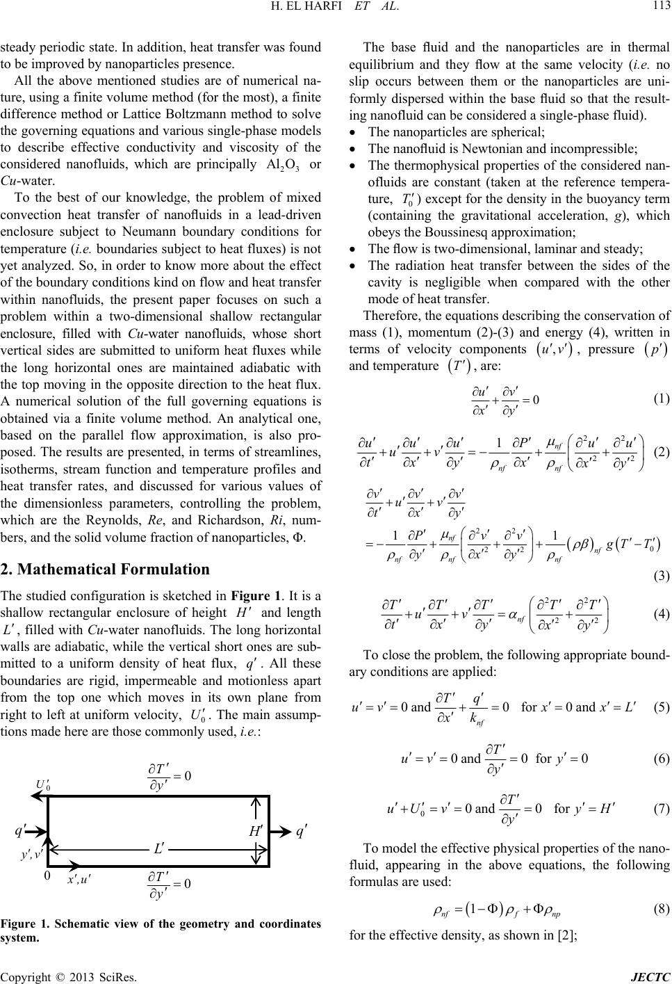 H. EL HARFI ET AL. 113 steady periodic state. In addition, heat transfer was found to be improved by nanoparticles presence. All the above mentioned studies are of numerical na- ture, using a finite volume method (for the most), a finite difference method or Lattice Boltzmann method to solve the governing equations and various single-phase models to describe effective conductivity and viscosity of the considered nanofluids, which are principally or Cu-water. 23 Al O To the best of our knowledge, the problem of mixed convection heat transfer of nanofluids in a lead-driven enclosure subject to Neumann boundary conditions for temperature (i.e. boundaries subject to heat fluxes) is not yet analyzed. So, in order to know more about the effect of the boundary conditions kind on flow and heat transfer within nanofluids, the present paper focuses on such a problem within a two-dimensional shallow rectangular enclosure, filled with Cu-water nanofluids, whose short vertical sides are submitted to uniform heat fluxes while the long horizontal ones are maintained adiabatic with the top moving in the opposite direction to the heat flux. A numerical solution of the full governing equations is obtained via a finite volume method. An analytical one, based on the parallel flow approximation, is also pro- posed. The results are presented, in terms of streamlines, isotherms, stream function and temperature profiles and heat transfer rates, and discussed for various values of the dimensionless parameters, controlling the problem, which are the Reynolds, Re, and Richardson, Ri, num- bers, and the solid volume fraction of nanoparticles, Φ. 2. Mathematical Formulation The studied configuration is sketched in Figure 1. It is a shallow rectangular enclosure of height H q and length , filled with Cu-water nanofluids. The long horizontal walls are adiabatic, while the vertical short ones are sub- mitted to a uniform density of heat flux, . All these boundaries are rigid, impermeable and motionless apart from the top one which moves in its own plane from right to left at uniform velocity, 0. The main assump- tions made here are those commonly used, i.e.: L U H L q q 0 y T 0 0 y T 0 U v ,y u,x Figure 1. Schematic view of the geometry and coordinates system. The base fluid and the nanoparticles are in thermal equilibrium and they flow at the same velocity (i.e. no slip occurs between them or the nanoparticles are uni- formly dispersed within the base fluid so that the result- ing nanofluid can be considered a single-phase fluid). The nanoparticles are spherical; The nanofluid is Newtonian and incompressible; The thermophysical properties of the considered nan- ofluids are constant (taken at the reference tempera- ture, 0 T ) except for the density in the buoyancy term (containing the gravitational acceleration, g), which obeys the Boussinesq approximation; The flow is two-dimensional, laminar and steady; The radiation heat transfer between the sides of the cavity is negligible when compared with the other mode of heat transfer. Therefore, the equations describing the conservation of mass (1), momentum (2)-(3) and energy (4), written in terms of velocity components , pressure ,uv p and temperature T , are: 0 uv xy (1) 22 22 1nf nf nf uuuPuu uv txy x x y (2) 22 0 22 11 nf nf nf nfnf vvv uv txy Pvv g TT yxy (3) 22 22 nf TTTTT uv txy xy (4) To close the problem, the following appropriate bound- ary conditions are applied: 0 and0for0 and nf Tq uvx xL xk (5) 0 and0for0 T uv y y (6) 00 and0for T uUvy H y (7) To model the effective physical properties of the nano- fluid, appearing in the above equations, the following formulas are used: 1 nff np (8) for the effective density, as shown in [2]; Copyright © 2013 SciRes. JECTC 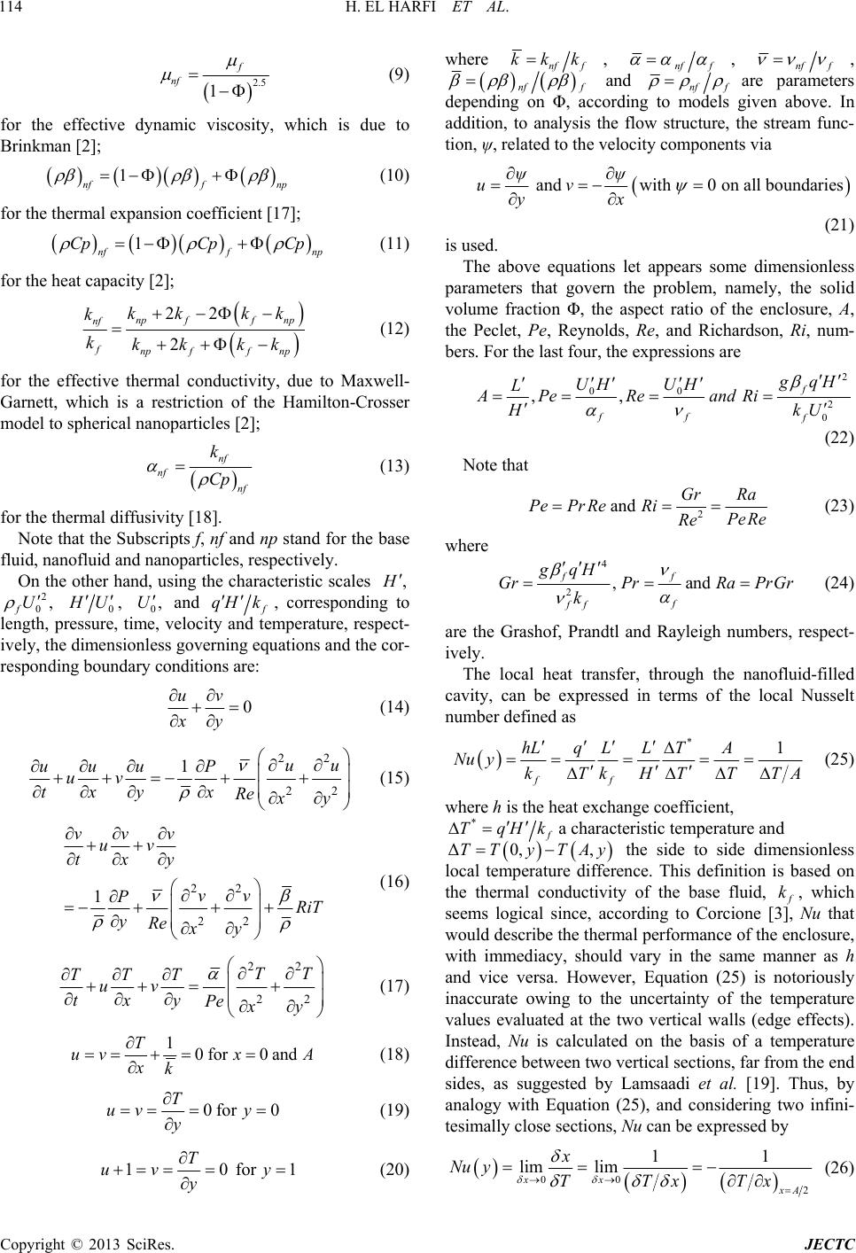 H. EL HARFI ET AL. 114 2.5 1 f nf (9) for the effective dynamic viscosity, which is due to Brinkman [2]; 1 nff np (10) for the thermal expansion coefficient [17]; 1 nff np CpCp Cp (11) for the heat capacity [2]; 22 2 npff np nf fnpff np kk kk k kkk kk (12) for the effective thermal conductivity, due to Maxwell- Garnett, which is a restriction of the Hamilton-Crosser model to spherical nanoparticles [2]; nf nf nf k Cp (13) for the thermal diffusivity [18]. Note that the Subscripts f, nf and np stand for the base fluid, nanofluid and nanoparticles, respectively. On the other hand, using the characteristic scales , H 2 0, fU 0, H U 0 and ,U f qH k , corresponding to length, pressure, time, velocity and temperature, respect- ively, the dimensionless governing equations and the cor- responding boundary conditions are: 0 uv xy (14) 22 22 1uu uuuP uv txy x Re x y (15) 22 22 1 vvv uv txy vv PRiT yRe xy (16) 22 22 TT TTT uv txy Pe x y (17) 10for 0and T uvx A xk (18) 0for 0 T uvy y (19) 10for T uv y y where nf f kkk, nf f , nf f , nf f and nf f are parameters depending on Φ, according to models given above. In addition, to analysis the flow structure, the stream func- tion, ψ, related to the velocity components via andwith0 on all boundaries ψψ u v yx (21) is used. The above equations let appears some dimensionless parameters that govern the problem, namely, the solid volume fraction Φ, the aspect ratio of the enclosure, A, the Peclet, Pe, Reynolds, Re, and Richardson, Ri, num- bers. For the last four, the expressions are 2 00 2 0 ,, f ff f g qH UH UH L APeReand Ri HkU (22) Note that 2 and Gr Ra PePrReRiPeRe Re (23) where 4 2,and ff f ff gqH GrPrRa PrGr k (24) are the Grashof, Prandtl and Rayleigh numbers, respect- ively. The local heat transfer, through the nanofluid-filled cavity, can be expressed in terms of the local Nusselt number defined as *1 ff hLq LLTA Nu ykTkHTTT A (25) where h is the heat exchange coefficient, * f TqHk a characteristic temperature and Δ0, ,TTyTAy the side to side dimensionless local temperature difference. This definition is based on the thermal conductivity of the base fluid, f k, which seems logical since, according to Corcione [3], Nu that would describe the thermal performance of the enclosure, with immediacy, should vary in the same manner as h and vice versa. However, Equation (25) is notoriously inaccurate owing to the uncertainty of the temperature values evaluated at the two vertical walls (edge effects). Instead, Nu is calculated on the basis of a temperature difference between two vertical sections, far from the end sides, as suggested by Lamsaadi et al. [19]. Thus, by analogy with Equation (25), and considering two infini- tesimally close sections, Nu can be expressed by 00 2 11 lim lim xx xA x Nu yTTxTx (26) 1 (20) Copyright © 2013 SciRes. JECTC  H. EL HARFI ET AL. 115 where x is the distance between two symmetrical sec- tions with respect to the central one. The corresponding average Nusselt number is calcu- lated, at different locations, from 1 NuNu y0dy (27) 3. Numerics 17) associated with Equations (18)-(20) Equations (14)-( have been solved by using a finite volume method and SIMPLER algorithm in a staggered uniform grid system [20]. A second order back-wards finite difference scheme has been employed to discretise the temporal terms ap- pearing in Equations (15)-(17). A line-by-line tridiagonal matrix algorithm with relaxation has been used in con- junction with iterations to solve the nonlinear discretised equations. The convergence has been considered as reached when 151 ,,, 10 kk k ij ijij ,,ij ij f ff , where , k ij f stands for the value of u, v, p or T at the kth iteration level and grid location (i, j) in the plane (x, y). The mesh size has been chosen so that a best compromise between run- ning time and accuracy of the results may be found. The procedure has been based on grid refinement until the numerical results agree, within reasonable accuracy, with the analytical ones, obtained from the parallel flow ap- proach developed in the next section. Hence, as shown in Table 1, a uniform grid size of 160 40 has been se- lected for 8A (value used for the numerical compu- tations) andeen estimated sufficient to model accu- rately the flow and temperature fields within the cavity. The time step size, t has b , has been varied in the range 74 10 10t , depeing on the values of the govern- 4. Approximate Parallel Flow nd ing parameters. Analytical As from Figures 2-4, displaying streamlines Solution can be seen (left) and isotherms (right), the flow and temperature fields exhibit a parallel aspect and a linear stratification, respectively, in the most part of the cavity, for 8 A and various values of Re, Ri and Φ. Accordingly, th- lowing simplifications e fol ,,uxy uy v,0,, and ,2 xy ψxy ψy TxyCxAθy (28) where C is unknown constant temperature gradient in the x-direction, are possible, which leads to the ordinary non- dimensional governing equations: 3 duT 3 dReRi ReRiC x y (29) Table 1. Accuracy tests conducted with Re = 1, 3 various values of . Ri = 10and Grids (160 20) Φ c Nu 0.0 0.4429 0 0.4179 3.6429 s (120 40) (200 4.720 0.1 0.2 0.3533 2.9500 Grid (160 40) 400) Φ c Nu c Nu c Nu 0.0 0.460.4427 4 0.0 0.41693.5940.4171 3.5952 0.41713.594 s 427 4.6444.6444428 4.644 0.1 89 0.2 0.35042.90180.3504 2.9024 0.35062.9018 Grid (160 60) Φ c Nu 0.0 0.4427 4 0.4179 3.5952 4.644 0.1 0.2 0.3502 2.9024 2 d 2 dCu Pe y (30) with dd 0for 0and 10for1 dd uyu yy y (31) as boundary, return tions, respectively. 1 0 d0uy y 1 (32) 0 d0yy flow and me (33) an temperature condi- Using such an approach, the solution of Equations (29) and (30), satisfying Equations (31)-(33), is 32 2 23 32 12 uyReRiC yyyyy (34) 543 2 43 11 121046 120 1 4330 yyy yRaC PeC y y The expression of the stream function, (35) ψ y , can be deduced by integration of Equation (21)nto ac- co nditi Eq , taking i unt of the corresponding boundary coons and uation (34), which gives: Copyright © 2013 SciRes. JECTC  H. EL HARFI ET AL. Copyright © 2013 SciRes. JECTC 116 (a (c) (b) ) (1) (b) (c) (a) (2) (b) (c) (a) (3) (a) (b) (c) (4) Figure 2. Streamlines (left) and isotherms (right) for Re = 0.1 ((a) = 0.1, (b) = 0.1 and (c) = 0.2) and Ri ((1) Ri = 1, (2) Ri = 10, (3) Ri = 102 and (4) Ri = 103). and various values of 42 yy 33 2 1222 yReRiCy yy (36) where . Therefore, the flow intensity is max min , cSup (37) where max and min are the extrema of ψ y at the cevertical section of the enclosure ntral 2xA. natuThey correspond tointensities of forced andral convections, respectively. the On the other hand, according to Bejan [21], the energy balance in x-direction is 111 dd TPe T yu Ty 0 or 000 xA xx In particular, in the pa d y (38) rallel flow region and with the application of Equation (18), Equation (38) becomes: 1 0k 1 d Pe Cuy (39) ves the following transcendental equation: which, when substituted to Equations (34) and (35), gi  H. EL HARFI ET AL. 117 (c) (b) (a) (1) (c) (b) (a) (2) (a) (c) (b) (3) (c) (b) (a) (4) Figure 3. Streamlines (left) and isotherms (right) for Re = 1 and various values of ((a) = 0.1, (b) = 0.1 and (c) 0.2) and Ri ((1) Ri = 1, (2) Ri = 10, (3) Ri = 102 and (4) Ri = 103). = 222 2 2 10 3360 362,880 105 CC C k (40) whose solution, via Newton-Raphson method, for Pe, Ra and Φ, leads to C. 3 1PePeRa Ra given Finally, taking into account of Equations (26) and (27), the Nusselt number is constant and can be expressed as 1 Nu NuC (41) 5. Results and Discussion With boundary conditions of Neumann kind (uniform heat flux imposed to vertical walls) the flow and thermal fields, and thermo-convective ch parallel, stratified and independent on the enclosure as- this parameter tends to aracteristics become pect ratio, A, respectively, when be large enough. In our situation, this has been occurred with 8 A in the limit of the explored values of Re 0.1 10Re , Ri 3 110Ri , 00.2 , and 7Pr (water based mixtures). Consequently, the Copyright © 2013 SciRes. JECTC  H. EL HARFI ET AL. 118 (b) (a) (c) (1) (b) (a) (c) (2) (b) (a) (c) (3) (b) (a) (c) (4) Figure 4. Streamlines (left) and isotherms (right) for Re = 10 and various values of ((a) = 0.1, (b) = 0.1 and (c) = 0.2) and Ri ((1) Ri = 1, (2) Ri = 10, (3) Ri = 102 and (4) Ri = 103). tours of streamlines (left) and isotherms (right) the flow is parallel to the horizontal boundaries and the temperature is linearly stratified in the horizontal direc- en from Figure 2 mixed convection flow developed within the enclosure is governed only by four dimensionless parameters, namely, e, Ri, in accordance with Equations (22)-(24), and are presented in Figures 2-4 for each Re and various Ri and Φ. First of all, remember that, except in the end sides, R possibly the type of nanoparticles, even if the present study is limited to Cu-water nanofluid, with the thermo- physical properties of Cu and water given in Table 2 [22]. The effects of these parameters on the flow and thermal fields and the resulting heat transfer will be now discussed. 5.1. Flow and Thermal Patterns Typical con tion. On the other hand, as can be se corresponding to Re = 0.1, the shear effect due to moving top wall is dominall (=1), relatively small (= ant for Ri sm 10) and moderate (=10²), since the flow is unicellular and counterclockwise with streamlines crowded near this boundary causing the lost of their own symmetry with respect to the horizontal mid-plane and this, whatever the value of Φ. In contrast, for relatively high Ri (=10³), a Copyright © 2013 SciRes. JECTC  H. EL HARFI ET AL. 119 clockwise cell, whose size reduces with an increasing Φ, is generated by buoyancy effect in the lower part of the cavity, i.e. under that due to lid-driven effect. The influ- ence of Φ can be explained by the fact that an increase of this parameter leads to an increase of the effective vis- cosity, which, in its turn, tends to decelerate the buoy- ancy flow and accelerate the shear one. In fact, the vis- cosity is a manifestation of surface phenomena and there- fore can only favour the shear flow. As for the isotherms, they remain almost vertical synonymous of pseudo-con- duction regime (i.e. low convection regime, Re = 0.1). An increase of Re to 1 (Figure 3) anticipates the buoy- ancy flow, since the related cell takes place at Ri = 10², with a decreasing size with Φ like before (i.e. Re = 0.1). However, such a cell tends to be large when passing to Ri = 10³, which is normal if one refer to Equation (22). In such a situation, the isotherms, which are tilted, with res- pect to y-axis, in the counterclockwise direction (i.e. that of the shear flow), gradually change direction of tilting as the buoyancy flow takes importance (i.e. while increas- ing Ri). But, with the presence of nanoparticles (i.e. with increasing Φ), such a change seems to occur slowly, de- pending on Ri. Finally, for Re = 10 (Figure 4), two small clockwise eddies develop in the bottom left and right cor- ners of the enclosure, for Ri = 10 (Figure 4(2a)), as a re- sult of buoyancy driven effect, although these structures may disappear wile introducing nanoparticles in the base fluid. As before, a progressive increase of Ri to 10² (Fig- ure 4(3)) makes stronger buoyancy effect and the two tiny eddies, observed previously, join each other and grow to give rise to a large buoyancy cell, whose size reduces slightly with Φ, for the reasons given above. A further increase of Ri to 10³ (Figure 4(4)) makes bigger enough buoyancy cell so that the effect of Φ, on this, cannot be detected, which is obvious since, according to Equation (22), inertia effects due to gravity prevail over those associated with top moving wall. At the same time, the isotherms appear to be nearly tilted in the direction of the strongest flow (shear flow for Ri = 1 and 10, and buoyancy flow for Ri = 10³). Between the two case, i.e. for Ri = 10², both the tendencies exist and the shape of the isotherms is strongly distorted. Here also, it is easy to see that an increase of Φ does not affect strongly the shape of isotherms. In addition to that, the similarity notion is not re- spected in the present problem since a change of Re may cause big changes in flow and thermal fields for given Ri Table 2. Thermophysical properties of base fluid (H2O) and nanoparticles (Cu) [22]. 3 kg m Jkg k P C Wmkk 5 101 k O 2 H 997.1 4179 0.613 21 Cu 8933 385 401 1.67 and Φ (compare, for example, Figures 2(3a)-4(3a) cor- responding to Ri = 102 and Φ = 0). Also, for the case Ri = 1, although buoyancy and lid-driven effects have the sam magnitude, th shear flows dominan because of thall depthe encl (shallow cavity). 5.2. Validaf the Aoximaarallew erature seen the two types of results is ee it e smth of osure tion opprte Pl Flo Analytical Solution In order to validate the approximate analytical solution, the numerical results (full circles) are compared to those obtained analytically (solid lines), as displayed in Fig- ures 5-7 giving stream function (left) and temp (right) profiles along the y-axis at the mid-length of the cavity, (A/2, y) and T(A/2, y), respectively. As can be , the agreement between quite perfect, which confirms the existence of an ana- lytical solution and validates mutually the parallel flow hypothesis and the elaborated computing code. Moreover, computed and calculated values of the stream function at the vertical central section of the cav- ity, c , and mean Nusselt number, Nu, presented in Figures 8-10, show also good agreement between the analytical and numerical results for a wide range of Ri, and various values of Re and Φ. 5. Se those discussed in sub- increase and natuhere Φ reost without influence due to mixing effects e extremum) corre- sp from the left hot side and cools the top (y = 1) after pass- 3. Stream Function and Temperature Distributions along the Vertical Central ction Although the results (Figures 5-7) of subsection 5.2 are related to the core region, where the parallel flow con- cept is valid, they confirm mostly section 5.1 and demonstrate that, in general, an of Φ amplifies and reduces the strengths of forced ral flows, respectively, except in some cases w mains alm that occur at Re = 10 (Figure 7). The presence of a maximum in the stream function profile indicates that the flow is unicellular counter- clockwise, driven mainly by the moving top wall. When this profile presents, simultaneously, two extrema, maxi- mum and minimum, this means that both the shear and buoyancy driven flows coexist and the flow regime is bicellular. The maximum (positiv onds to shear flow, which is counterclockwise, and the minimum (negative extremum) is related to buoyancy flow that is clockwise. Generally, the temperature profile presents two or three zones with positive and negative signs, namely (+,−), (−,+,−) and (−,+), depending on the flow nature and the competition between lid and buoyancy driven effects. Thus, with a dominant lid-driven effect, the shear flow warms the bottom (y = 0) by transporting the heat Copyright © 2013 SciRes. JECTC  H. EL HARFI ET AL. Copyright © 2013 SciRes. JECTC 120 0.16 0.02 0.04 0.0 0.2 0.4 0.6 0.8 1.0 0.00 0.04 0.08 0.12 Ri = 1 Analytical solution Numerical solution = 0.0 = 0.1 = 0.2 y0.0 0.2 0.4 0.6 0.8 1.0 -0 .0 4 -0 .0 2 0.00 TAnalytical solution Numerical solution = 0.0 = 0.1 Ri = 1 = 0.2 y 0.0 0.2 0.4 0.6 0.8 1.0 0.00 0.04 0.08 0.12 0.16 Analytical solution Numerical solution = 0.0 = 0.1 = 0.2 Ri = 10 y0.0 0.2 0.4 0.6 0.8 1.0 -0.04 -0.03 -0.02 -0.01 0.00 0.01 0.02 0.03 Numerical solution = 0.0 = 0.1 = 0.2 Analytical solution Ri = 10 T y 0.0 0.2 0.4 0.6 0.8 1.0 0.00 0.03 0.06 0.09 0.12 0.15 Numerical solution = 0.0 = 0.1 = 0.2 Analytical solution Ri = 102 y0.0 0.2 0.4 0.6 0.8 1.0 -0.03 -0.02 -0.01 0.00 0.01 0.02 Analytical solution Numerical solution = 0.0 = 0.1 = 0.2 Ri = 102 T y 0.0 0.2 0.4 0.6 0.8 1.0 -0.15 -0.10 -0.05 0.00 0.05 0.10 0.15 Analytical solution Numerical solution = 0.0 = 0.1 = 0.2 Ri = 103 y0.0 0.2 0.4 0.6 0.8 1.0 -0.03 -0.02 -0.01 0.00 0.01 0.02 Numerical solution = 0.0 = 0.1 = 0.2 Ri = 103 Analytical solution T y Figure 5. The stream function (left) and temperature (right) profiles at mid-length of the cavity, along the vertical coordinate, for Re = 0.1 and various values of and Ri.  H. EL HARFI ET AL. 121 0.0 0.2 0.40.6 0.8 1.0 0.00 0.04 0.08 0.12 0.16 Ri = 1 Analytical solution Numerical solution = 0.0 = 0.1 = 0.2 y0.0 0.2 0.4 0.6 0.8 1.0 -0.3 -0.2 -0.1 0.0 0.1 0.2 Ri = 1 Analytical solution Numerical solution = 0.0 = 0.1 = 0.2 T y 0.0 0.2 0.4 0.6 0.8 1.0 -0.02 0.00 0.04 0.08 0.12 0.16 Analytical solution Numerical solution = 0.0 = 0.1 = 0.2 Ri = 10 y0.0 0.2 0.40.6 0.8 1.0 -0.25 -0.20 -0.15 -0.10 -0.05 0.00 0.05 0.10 0.15 Analytical solution Numerical solution = 0.0 = 0.1 = 0.2 Ri = 10 T y 0.0 0.2 0.40.6 0.8 1.0 -0.12 -0.08 -0.04 0.00 0.04 0.08 0.12 Numerical solution = 0.0 = 0.1 = 0.2 Analytical solution Ri = 102 y0.0 0.2 0.40.6 0.8 1.0 -0.15 -0.10 -0.05 0.00 0.05 0.10 0.15 Analytical solution Numerical solution = 0.0 = 0.1 = 0.2 Ri = 102 T y 0.0 0.20.4 0.6 0.81.0 -0.2 -0.1 0.0 0.1 0.2 Numerical solution = 0.0 = 0.1 = 0.2 Analytical solution Ri = 103 T y 0.0 0.20.4 0.6 0.8 1.0 -0.5 -0.4 -0.3 -0.2 -0.1 0.0 0.1 Analytical solution Numerical solution = 0.0 = 0.1 = 0.2 Ri = 103 y Figure 6. The stream function (left) and temperature (right) profiles at mid-length of the cavity, along the vertical coornate, for Re = 1 and various values of and Ri. di Copyright © 2013 SciRes. JECTC  H. EL HARFI ET AL. 122 0.06 0.16 0.0 0.2 0.4 0.6 0.8 1.0 -0.02 0.00 0.04 0.08 0.12 Ri = 1 Analytical solution Numerical solution = 0.0 = 0.1 = 0.2 y0.0 0.2 0.4 0.6 0.8 1.0 -0. 0 9 -0. 0 6 -0. 0 3 0.00 0.03 Analytical solution Ri = 1 Numerical solution = 0.0 = 0.1 = 0.2 T y 0.0 0.2 0.4 0.6 0.8 1.0 -0.02 0.00 0.04 0.08 0.12 0.16 Numerical solution = 0.0 = 0.1 = 0.2 Analytical solution Ri = 10 y0.0 0.2 0.4 0.6 0.8 1.0 -0.08 -0.04 0.00 0.04 0.08 Analytical solution Numerical solution = 0.0 = 0.1 = 0.2 Ri = 10 T y 0.0 0.2 0.4 0.6 0.8 1.0 -0.09 -0.06 -0.03 0.00 0.03 0.06 Analytical solution Numerical solution = 0.0 = 0.1 = 0.2 Ri = 102 y0.00.20.40.60.81.0 -0.10 -0.05 0.00 0.05 0.10 Analytical solution Numerical solution = 0.0 = 0.1 = 0.2 Ri = 102 T y 0.0 0.2 0.4 0.6 0.8 1.0 -0.25 -0.20 -0.15 -0.10 -0.05 0.00 0.05 0.10 Numerical solution = 0.0 = 0.1 = 0.2 Analytical solution Ri = 103 y0.0 0.2 0.4 0.6 0.8 1.0 -0.050 -0.025 0.000 0.025 0.050 Analytical solution Numerical solution = 0.0 = 0.1 = 0.2 Ri = 103 T y Figure 7. The stream function (left) and temperature (right) profiles at mid-length of the cavity, along the vertical coordinate, for Re = 10 and various values of and Ri. Copyright © 2013 SciRes. JECTC  H. EL HARFI ET AL. Copyright © 2013 SciRes. JECTC 123 0 . 7 0.0015001000 1500 2000 25003000 0.0 0.1 0.2 0.3 0.4 0.5 0.6 (a) Analytical solution Numerical solution = 0.2 = 0.1 = 0.0 Ri c 0.0015001000 15002000 2500 3000 0.9 1.0 1.1 1.2 1.3 1.4 1.5 1.6 1.7 1.8 Analytical solution Numerical solution (b) = 0.2 = 0.1 = 0.0 Nu Ri Figure 8. Flow intensity (a) and heat transfer rate (b) versus Ri, for Re = 0.1 and various values of . ing near the right cold side. This is the case of a tem- perature profile of signs (+,−). With competing shear and buoyancy flows, the temperature sign is such that the corresponding counterclockwise and clockwise cells act so that the interface between them is warm, the bottom is cold and the top is warm (−,+) or cold (−,+,−) depending on whether shear or buoyancy effect is dominant, and on Φ. 5.4. Flow Intensity and Heat Transfer Rate For further analysis of the problem, the flow intensity (top), , and heat transfer rate (bottom), Nu c , are re- ported, against Ri, in Figures 8-10, for each Re and var- ious Φ. It is easy to observe that c depen a dec exhibits in general two tendencies, whose expanseds on Re and Φ. The first one is characterized byrease of c with Ri, expressing a reduction of thrength of tear flow until a minimum reached at particular value Ri, which increases and decreases with and Re, respectively. The second one corresponds toncrease of e st Φ an i he sh of c with Ri, beyond the minimum obserd, and expr aug- veesses an  H. EL HARFI ET AL. 124 0.5 0.001200 400 600 8001000 0.0 0.1 0.2 0.3 0.4 (a) = 0.2 = 0.1 = 0.0 Ri c Analytical solution Numerical solution 0.001200 400 600 8001000 0 1 2 3 4 5 (b) Analytical solution Numerical solution = 0.2 = 0.1 = 0.0 Nu Ri Figure 9. Flow intensity (a) and heat transfer rate (b) versus Ri, for Re = 1 and various values of . mentation of the strength of the buoyancy flow which reduces with Φ. It can be seen, also, that an increase of Re leads, first, to an increase of c and, second, to a decrease of this quantity (compare Figures 8-10, ob- tained for Re = 0.1, 1 and 10, respectively). This is due, probably, to a change of the dominant role from one re- gime to another. With regard to Nu , a slight increase of this quantity, with Ri, is observed for Φ = 0, but such a tendency dis- appears, as Φ increases, leading to a constant . This behaviour is the consequence of an increase of the effect- e mo- ion is of Nu ive viscosity with Φ, which acts to slow down th tion, particularly, for Re = 0.1 where mixed convect weak (Figure 8). Moreover, for Re = 1 and 10, two trends evolution appear for Nu , as foc r , since Nu decreases and increases with Ri on both sides of a minimum depending on Φ (Figures 9 and 10e first tre driven flow. In contrast, the second trend, whiretches ). Th ch st nd, which corresponds to a short range of Ri, whose expanse increases with Φ, is related to a dominant lid- Copyright © 2013 SciRes. JECTC  H. EL HARFI ET AL. 125 0.25 0.001 2004006008001000 0.05 0.10 0.15 0.20 (a) Analytical solution Numerical solution = 0.2 = 0.0 = 0.1 Ri c 0.001200400 600 8001000 0 20 40 60 80 (b) Analytical solution Numerical solution = 0.2 = 0.1 = 0.0 Nu Ri Figure 10. Flow intensity (a) and heat transfer rate (b) versus Ri, for Re = 10 and various values of . over a large range of Ri, is associated with a prevailing buoyancy-driven flow. Last, Figures 8-10 show also the quite obvious increase of Nu with Re, conveying the favorable role of the lid-driven flow to heat transfer. In order to examine the influence of Φ on flow inten- sity and heat transfer rate, the quantities c (top) and Nu (bottom) are plotted against Φ for various Ri and each Re, in Figures 11-13. For Re = 0.1 (Figure 11), except for Ri = 103 where a decrease of c , with Φ, due probably to the reduction of buoyancy effect by nanopar- are, in general, increasing functions of Φ. For Re = 1, Figure 12 shows different variations of c and Nu , with Φ, de- ticles, is observed for Φ < 7.5%, c andNu pending on Ri. Hence, for Ri = 1 and 10, c is almost constant (very weak slop), ncreawhile the ise of Nu is is not notabr Ri = , clear, although itle. Fo10² c pre- send nts a decrease aan increase on both sides of Φ = 6.25%, whereas the increase of Nu is monotonic. For Ri = 10³ the tendency is reversed since c andNu are decreasing functions of Φ. At last, for Re = 10 (Fig- ure 13), c seems to be quite unconcerned about any variatioΦ n of , whilst Nu undconsta c nt ergoes Copyright © 2013 SciRes. JECTC  H. EL HARFI ET AL. 126 0.14 0.16 0.00 0.02 0.040.06 0.08 0.10 0.120.14 0.16 0.18 0.20 0.00 0.02 0.04 0.06 0.08 0.10 0.12 Ri = 1 Ri = 102 Ri = 10 Analytical solution (a) Numerical solution Ri = 103 c 0.00 0.02 0.04 0.06 0.08 0.10 0.12 0.14 0.16 0.18 0.20 1 1.2 1.5 1.8 (b) Ri = 1,10,102,103 Analytical solution Numerical solution Nu Figure 11. Flow intensity (a) and heat transfer rate (b) versus , for Re = 0.1 and various values of Ri. a diminution with this parameter, at least for the selected values of Ri. It is clear fluids lead to contradictory conclusions, depending on uall ven flo happens, which is paradoxical when nanoflds are ex- pected to improve heat transfer. This can be related, es- nductivity and v that the results related to heat transfer in nan- sentially, to the conflict between effective co o the flow nature, thus leaving still unanswered the ques- tion if the use of nanoparticle suspensions for mixed con- vection applications is acty advantageous with re- spect to pure liquids. In fact, with dominant lid-dri w, heat transfer enhances with nanoparticles, whereas with dominant buoyancy-driven flow the opposite effect iscosity with the complicity of the cavity aspect ratio, which is large and favours the effect of viscosity and disfavours that of conductivity. 5.5. Onset of the Bicellular Flow In Figure 14 is depicted the evolution of c Ri , corre- ui Copyright © 2013 SciRes. JECTC  H. EL HARFI ET AL. 127 0.4 0.5 0.00 0.02 0.04 0.06 0.08 0.10 0.12 0.14 0.16 0.18 0.20 0.0 0.1 0.2 0.3 Ri = 1 (a) Analytical solution Numerical solution Ri = 103 Ri = 102 Ri = 10 c 0.00 0.02 0.04 0.06 0.080.10 0.12 0.14 0.16 0.18 0.20 1.0 1.5 2.0 2.5 3.0 3.5 4.0 4.5 5.0 Ri = 1 Ri = 102 Ri = 10(b) Ri = 103 Analytical solution Numerical solution Nu Figure 12. Flow intensity (a) and heat transfer rate (b) versus , for Re = 1 and various values of Ri. sponding to the onset of buoyancy-driven flow, which gives rise to bicellular flow, versus Re, for various values of Φ. As can be seen, decreases and increases on both sides alue, , of Re suc, depending on flow tends s precocious, so the presence of nanoparticles delays the onset of buoy- ancy-driven flow and then opposes to the corresponding effect, confirming the deterioration observed, efore, for c Ri h that to of a minimum corresponding to a particular heat transfer associated with this kind of flow. vm Φ. This trend indicates that the appearance of the buoy- ancy-driven Re 15 m Re be sometime metimes late around m Re . In addition to that, the more Φ increases the more c Ri increases, which means that 6. Conclusions In this paper, a numerical and analytical study on mixed convection in a two-dimensional horizontal shallow b Copyright © 2013 SciRes. JECTC  H. EL HARFI ET AL. 128 0.25 0.00 0.02 0.040.06 0.08 0.10 0.12 0.14 0.16 0.18 0.20 0.05 0.10 0.15 0.20 Ri = 1 (a) Analytical solution Numerical solution c Ri = 103 Ri = 102 Ri = 10 0.00 0.02 0.04 0.06 0.08 0.100.120.140.16 0.18 0.20 5 10 20 30 40 50 60 70 80 90 Ri = 10 Ri = 102 Ri = 1 (b) Ri = 103 Analytical solution Numerical solution Nu Figure 13. Flow intensity (a) and heat transfer rate (b) versus , for Re = 10 and various values of Ri. enclosure, of aspect ratio , filled with a nanofluid, has been conducted in the case where both short vertical sides are submitted to uniform heat fluxes while the long horizontal ones are assumed adiabatic, with the top one uniformly moving in the opposite direction to heat flux. The full partial differential equations, governing the problem, ha olume method. The computations, which have been lim- respectively, in the ranges, 0 and .2 8A ve been solved numerically using a finite v ited to Cu-water mixtures, with 7Pr , have been car- ried out with governing parameters, Re, Ri and Φ, varying, 0.1 10Re 3 11Ri 00 s of a paralle nclosure. be summar In the limit o numerical ones . Analytice basi l flow assu the eThe main findi can ized as follows f the selected th , which al solution is d mption in the ngs of such an : values of validates mutually bot rived on the core region of investigation e governing ell with the h the cor- parameters, analytical results, agree very w responding approaches. Flow and temperature fields strongly depend on the Copyright © 2013 SciRes. JECTC  H. EL HARFI ET AL. 129 103 0.1 110 10 102 Analytical solution Numerical solution = 0.0 Re Figure 14. Limit of the onset of the bicellular flow, for various values of . Richardson number, measuring the relative impor- tance of both lid and buoyancy-driven effects. Increasing the Richardson number is, in general, as- sociated with decreasing of heat transfer rate due to shear flow and increasing of that due to buoyancy- driven flow. The addition of Cu-nanoparticles into the pure water leads to an enhancement of lid-driven convection heat transfer. Against all odds, the addition of Cu-nanoparticles into the pure water results in a degradation of buoyancy- driven convection heat transfer. Therefore, although prospects of nanofluids are very promising, there is still a dearth of enough research in this area. The onset of buoyancy-driven flow, giving rise to bi- cellular flow, depends strongly on the Reynolds num- ber and nanoparticles volume fraction. REFERENCES [1] S. U. S. Choi, “Enhancing Thermal Conductivity of Flu- ids with Nanoparticles,” In: D. A. Siginer and H. P. Wang, Eds., Developments and Applications of Non-Newtonian Flows, American Society of Mechanical Engineers, New York, 1995, pp. 99-105. [2] W. Yu, D. M. France, S. U. S. Choi and J. L. Routbort, “Review and Assessment of Nanofluid Technology for Transportation and Other Applications,” Technical Report ANL/E Systems Division, Argonne, 2007. dge Driven Nanofluids inside Rectangular Enclosures Differ- entially Heated at the Sidewalls,” International Journal of Thermal Sciences, Vol. 49, No. 9, 2010, pp. 1536-1546. doi:10.1016/j.ijthermalsci.2010.05.005 = 0.1 Ric = 0.2 [4] L. A. B. Pilkington, “Review Lecture. The Float Glass Process,” Proceedings of the Royal Society of London. Series A, Mathematical and Physical Scienc, Vol. 314, No. 1516, 1969, pp. 1-25. doi:10.1098/rspa.1969.0212 SD/07-9, Argonne National Laboratory, Energy http://www.osti.gov/bri [3] M. Corcione, “Heat Transfer Features of Buoyancy- es [5] F. J. K Ideriah, “Prediction of Turbulent Cavity Flow Driven by Buoyancy and Shear,” Journal of Mechanical Engineering Sciences, Vol. 22, No. 6, 1980, pp. 287-295. doi:10.1243/JMES_JOUR_1980_022_054_02 [6] J. Imberger and P. F. Hamblin, “Dynamics of Lakes, Res- ervoirs, and Cooling Ponds,” Annual Review of Fluid Mechanics, Vol. 14, 1982, pp. 153-187. doi:10.1146/annurev.fl.14.010182.001101 [7] C. K. Cha and Y. Jaluria, “Recirculating Mixed Con- vection Flow for Energy Extraction,” International Jour- nal of Heat Mass Transfer, Vol. 27, No. 10, 1984, pp. 1801-1810. doi:10.1016/0017-9310(84)90162-5 [8] R. K. Tiwari and M. K. Das, “Heat Transfer Augmenta- tion in a Two-Sided Lid-Driven Differentially Heated Square Cavity Utilizing Nanofluids,” International Jour- nal of Heat and Mass Transfer, Vol. 50, No. 9-10, 2007, pp. 2002-2018. doi:10.1016/j.ijheatmasstransfer.2006.09.034 [9] E. Abu-Nada and A. J. Chamkha, “Mixed Convection Flow in a Lid-Driven Square Enclosure Filled with a Nanofluid,” European Journal of Mechanic Fluids, Vol. 29, No. 6, 2010, pp. 472-482. B/ doi:10.1016/j.euromechflu.2010.06.008 [10] M. Mahmoodi, “Mixed Convection inside Nanofluid Filled Rectangular Enclosures with Moving Bottom Wall,” International Journal of Thermal Sciences, Vol. 15, No. 3, 2011, pp. 889-903. Copyright © 2013 SciRes. JECTC  H. EL HARFI ET AL. 130 doi:10.2298/TSCI101129030M [1 d,” Inte 1] M. A. Mansour, R. A. Mohamed, M. M. Abd-Elaziz and S. E. Ahmed, “Numerical Simulation of Mixed Convec- tion Flows in a Square Lid-Driven Cavity Partially Heat- ed from below Using Nanofluirnational Commu- nication in Heat and Mass Transfer, Vol. 37, No. 10, 2010, pp. 1504-1512. doi:10.1016/j.icheatmasstransfer.2010.09.004 [12] M. Muthtamilselvan, P. Kandaswamy and J. Lee, “Heat Transfer Enhancement of Copper-Water Nanofluids in a Lid-Driven Enclosure,” Communications in Nonlinear Science and Numerical Simulation, Vol. 15, No. 6, 2010, pp. 1501-1510. doi:10.1016/j.cnsns.2009.06.015 [13] H. Nemati, M. Farhadi, K. Sedighi, E. Fattahi and A. A. R. Darzi, “Lattice Boltzmann Simulation of Nanofluid in Lid-Driven Cavity,” International Communication in Heat and Mass Transfer, Vol. 37, No. 10, 2010, pp. 1528- 1534. doi:10.1016/j.icheatmasstransfer.2010.08.004 [14] F. Talebi, A. H. Mahmoudi and M. Shahi, “Numerical Study of Mixed Convection Flows in a Square Lid- Driven Cavity Utilizing Nanofluid,” International Com- munication in Heat and Mass Transfer, Vol. 37, No. 1, 2010, pp. 79-90. doi:10.1016/j.icheatmasstransfer.2009.08.013 [15] G. A. Sheikhzadeh, N. Hajialigol, M. E. Qomi and A. Fattahi, “Laminar Mixed Convection of Cu-Water Nano- fluid in Two Sided Lid-Driven Enclosures,” Journal of Nanostructures, Vol. 1, No. 1, 2012, pp. 44-53. [16] M. A. Karimipour and M. M. Bazofti, “Periodic Mixed Convection of a Nanofluid in a Cavity with Top Lid Si- ol. 1, No. 1, 2010, pp. 34- nusoidal Motion,” International Journal of Mechanical and Materials Engineering, V 39. [17] Y. Xuan and W. Roetzel, “Conceptions for Heat Transfer Correlation of Nanofluids,” International Journal of Heat and Mass Transfer, Vol. 43, No. 19, 2000, pp. 3701-3707. doi:10.1016/S0017-9310(99)00369-5 18] E. B. Ogut, “Natural Convection of Water-Based Nano- [ fluids in an Inclined Enclosure with a Heat Source,” In- ternational Journal of Thermal Sciences, Vol. 48, No. 11, 2009, pp. 2063-2073. doi:10.1016/j.ijthermalsci.2009.03.014 [19] M. Lamsaadi, M. Naimi and M. Hasnaoui, “Natural Con- vection Heat Transfer in Shallow Horizontal Rectangular Enclosures Uniformly Heated from the Side and Filled with Non-Newtonian Power Law Fluids,” Energy Con- version and Management, Vol. 47, No. 15-16, 2006, pp. 2535-2551. doi:10.1016/j.enconman.2005.10.028 [20] S. Patankar, “Numerical Heat Transfer and Fluid Flow,” Hemisphere, Washington DC, 1980. [21] A. Bejan, “The Boundary Layer Regime in a Porous Layer with Uniform Heat Flux from Side,” International Journal of Heat Mass Transfer, Vol. 26, No. 9, 1983, pp. 1339-1346. doi:10.1016/S0017-9310(83)80065-9 [22] E. Abu-Nada, Z. Masoud and A. Hijazi, “Natural Con- vection Heat Transfer Enhancement in Horizontal Con- centric Annuli Using Nanofluids,” International Commu- nication in Heat and Mass Transfer, Vol. 35, No. 5, 2008, pp. 657-665. doi:10.1016/j.icheatmasstransfer.2007.11.004 Copyright © 2013 SciRes. JECTC |