Journal of Electronics Cooling and Thermal Control, 2013, 3, 101-110
http://dx.doi.org/10.4236/jectc.2013.33012 Published Online September 2013 (http://www.scirp.org/journal/jectc)
Second Law Analysis of Forced Convective Cooling i n a
Channel with a Heated Wall Mounted Obstacle
Z. Kheirandish, S. A. Gandjalikhan Nassab*, M. Vakilian
Mechanical Engineering Department, Shahid Bahonar University, Kerman, Iran
Received May 18, 2013; revised June 18, 2013; accepted June 25, 2013
Copyright © 2013 Z. Kheirandish et al. This is an open access article distributed under the Creative Commons Attribution License,
which permits unrestricted use, distribution, and reproduction in any medium, provided the original work is properly cited.
ABSTRACT
The present work details a numerical simulation of forced convective laminar flow in a channel with a heated obstacle
attached to one wall. The second law analysis is employed to investigate the distribution of entropy generation in the
flow domain to demonstrate the rate of irreversibilities in thermal system. The conjugate problem including the convec-
tion heat transfer in the fluid flow and conduction one inside the obstacle is solved numerically to obtain the velocity
and temperature fields in both gas and solid phases. To reach this goal, the set of governing equations including mo-
mentum and energy equations for the gas phase and conduction equation for the obstacle are solved by CFD technique
to determine the hydrodynamic and thermal behaviors of the fluid flow around the obstacle and the temperature distri-
bution in the solid element. An attempt is made to detail the local Nusselt number distribution and mean Nusselt num-
ber and also the local entropy generation distribution for the individual exposed obstacle faces. A good consistency is
found between the present numerical results with experiment.
Keywords: Conjugated Heat Transfer; Obstacle; Forced Convection Flow; Entropy Generation
1. Introduction
In many thermal systems, convection flow is concerned
to procure the precise thermal control. Besides, in heat
exchange devices, high performance, light weight and
compact heat transfer components are design scope. To
achieve these goals, extended surfaces are widely used in
heat exchange devices and the design of optimized fins
has become increasingly important nowadays. There
were numerous studies on fins performance and it has
found out that fins increase the rate of convection heat
transfer by increasing in fluid mixing and also interrupt-
ing the development of thermal boundary layer on the
heated surfaces.
Several researchers studied heat transfer enhancement
in forced convection duct flow using obstacles with dif-
ferent shapes. Young and Vafai [1,2] focused on special
selection of obstacle size and thermal conductivity and
found out those significant positive effects of them on the
flow and heat transfer characteristics. They numerically
studied heated square fin on 2-D laminar flow by finite
element method. Also they did an experimental study to
find the effect of one, three and five fins on the fluid flow
behavior in a wide range of the Reynolds numbers [3].
Chen and Huang [4] studied position of fins and their
arrangement. They investigated force convection cooling
of fin arrays in a 2-D channel flow and concluded more
mixing in fluid causes an increase in convective heat
transfer rate.
Numerical techniques in solving the set of governing
equations have special role on results accuracy and re-
quired run time. In the related subject, Carvalho et al. [5]
did a theoretical study for convection cooling in duct
flow. They compared different schemes by analyzing
hydraulic behavior of laminar flow in a channel with
mounted obstacle and found that quadratic upstream
scheme has the most advantageous regarding accuracy
against computing time and storage space.
Chen et al. [6] did an experimental research on 3-D
channel flow with drop shape fin. It was reported in their
paper that the drop shape fin has better thermal perform-
ance than circular one.
In another research, Korichi and Oufer [7] studied on
channel containing mounted obstacles, in which two ob-
stacles mounted on the lower wall and the last one on the
upper wall of a 2-D channel. They investigated a nu-
merical study on laminar convective flow and studied the
*Corresponding author.

Z. KHEIRANDISH ET AL.
102
effect of Reynolds number, block spacing and dimen-
sions and also solid to fluid thermal conductivity ratio.
Their results showed that increasing in Reynolds number
causes more heat removal from the obstacles. Also, it
was revealed that maximum heat removal occurred
around the obstacle corners.
Li et al. [8] carried out an experiment to investigate
the hydrodynamic and thermal behaviors of forced con-
vection flow in rectangular channel with staggered arrays
of elliptic and circular fins. Their results showed that the
rate of cooling by the elliptic fin is more than that of cir-
cular one.
On the other hand, the optimum condition for any
process can be determined by the entropy generation ana-
lysis because one of the primary objectives in the design
of any energy system is to conserve the useful energy
applied to take place a certain process. The ireversibili-
ties associated within the process components destroy the
useful energy. It is clear that using fins in convection
cooling system increases the amount of irreversibilities.
Because of the second law of thermodynamics, irreversi-
bility can not be avoided completely but it can be mini-
mized in order to save the available energy. The present
work also deals with the second law analysis in convec-
tion duct flow with fin to carry out the rate of irreversi-
bilities due to the presence of obstacle.
In the related subject, Bejan [9] obtained a systematic
methodology to calculate irreversibility through fluid
flow and heat transfer in heat exchangers. Chen et al. [10]
studied transverse fin in laminar forced convection chan-
nel flow and analyzed entropy generation. They used
vorticity stream function method to solve the continuity
and momentum equations for fluid flow. They found that
fins increase the rates of irreversibilities, both due to vis-
cous effect and irreversible heat transfer process, al-
though they disturb developing of thermal boundary lay-
er which leads to heat transfer enhancement.
In several researches, entropy generation were studied
in detail for different flow and channel conditions. Ko et
al. [11] carried out a numerical study on wavy channel to
investigate entropy generation of laminar forced convec-
tion flow (Re = 100 up to 400). Their studies showed that
for high Reynolds number convection flows, irreversi-
bilities are minimums when duct width to height ratio is
equal to unity. In another study, they numerically ana-
lyzed entropy generation produced by a forced convec-
tive flow in a curved rectangular duct with external heat-
ing [12]. Three important factors such as Dean number,
external wall heat flux and cross-sectional aspect ratio on
entropy generated from frictional irreversibility and heat
transfer irreversibility were investigated in detail. It was
shown that, at larger Dean number and smaller wall heat
flux, frictional irreversibility is the most impressive
source of entropy generation; whereas and vice versa,
condition for Dean number and wall heat flux, the en-
tropy generation is dominated by heat transfer irreversi-
bility. Also, Ko [13] investigated the effect of longitudi-
nal ribs on laminar forced convection and entropy gen-
eration in a curved rectangular duct. He found that the
number of mounted ribs and their arrangement have in-
fluential effect on flow characteristics and temperature
distributions. Ko et al. [14] did a numerical study on en-
tropy generation by turbulent forced convective flow in a
curved rectangular duct with various aspect ratios. It was
found that the duct aspect ratio has great effect on the
distribution of local entropy generation number through
the flow domain.
Although there are many studies about numerical ana-
lysis of convective cooling in channel and also about the
analysis of such thermal systems by computing the en-
tropy generation, a careful inspection of literatures shows
that the entropy generation analysis in convective cooling
duct flow with obstacles that leads to a conjugate prob-
lem is still not studied. Therefore, the present research
deals with the investigation of entropy generation in a
forced convection flow adjacent to an obstacle in a duct
with conjugate problem for the fist time. Toward this end,
the set of governing equations consists of the continuity,
Navier-Stokes and energy equations for the fluid flow
and conduction equation for the obstacle are solved nu-
merically by the CFD method. Because the Cartesian co-
ordinate system is used for this computation, the block
off method is employed for simulating the obstacle in the
computational domain.
2. Theory
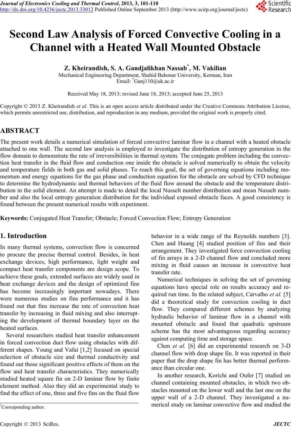
Computational domain of the problem is shown in Fig-
ure 1. Laminar convective flow enters a 2-D channel
which a heated obstacle mounted on bottom wall. Fluid
has uniform temperature Tin and parabolic velocity at the
inlet of channel. The duct walls are kept insulated except
the lower edge of fin which is maintained at constant
temperature Tw which is more than fluid inlet tem-
perature.
The height of the duct is H and the lengths of the duct
upstream and downstream sides of the fin are Li and Le,
respectively. This is made to ensure that the flows at the
inlet and outlet sections are not affected significantly by
the sudden change in the geometry and flow at the exit
section becomes fully developed. The height and width
of the fin are denoted by L and D such that L = D = 0.25
H is considered in all of the subsequent calculations.
3. Basic Equations
The non-dimensional governing equations which are the
conservations of mass, x- and y-momentum and energy
for fluid flow in the Cartesian coordinate can be written

Z. KHEIRANDISH ET AL.
103
Tin
u(y)
Adiabatic wall Adiabatic wall
Adiabatic wall
Solid
fin
Tw Li
L
D
Le
H
Lt
Figure 1. Schematic of the computational domain.
as follows:
0
UV
XY


 (1)
211UUP
UUV
XXYReRe YX

 

 

 
(2)
2
11VVP
UV V
XXYReRe YY






(3)
1Θ1Θ
ΘΘ0UV
XPeXYPeY






(4)
For solid phase, the conduction equation is considered
as follows:
22
22
ΘΘ
0
XY






(5)
In the above equations, the dimensionless parameters
are defined as:
 
00
0
2
0
,,,, ,,,
,,,
in
win
TT xyu v
XY UV
H
HUUTT
UH
p
PRe PrPeRePr
U



 



 
 
 
(6)
4. Boundary Conditions
As mentioned above, fully developed gas flow with par-
abolic profile and uniform ambient temperature Tin enters
the channel. Channel walls are insulated except the ob-
stacle lower wall which is imposed on constant tem-
perature of Tw. The adiabatic wall condition is selected to
elucidate the principal aspects of parametric changes in
the heated obstacle to the flow and thermal fields within
the channel. On all solid surfaces, no-slip condition is
employed for velocity. At the outlet section, zero axial
gradients for velocity components and fluid temperature
are applied. Finally on the solid-gas interfaces, the con-
tinuity of temperature and heat flux is considered that
leads to the following equations:
f
s


f
s
sf
kk
nn

 

 (7)
The value of local Nusselt number on the heated sur-
faces can be calculated as follows:

1Θ
ΘΘ
c
fsm
hh
Nu kn


(8)
In this formula, n is normal direction to the heated
surface and m

is the fluid mean temperature which is
determined according to the following equation:
1
ΘΘd
mHY
UH
 (9)
The mean values of Nusselt number on each obstacle
walls can be calculated by [2]:
d
ix
A
i
i
Nux
Nu A  (10)
Subsequently, the value of mean Nusselt number on
the obstacle surface which is exposed to the fluid flow is
calculated as follow [2]:
,, ii iltr
m
ltr
Nu A
Nu
A
AA




 (11)
5. Entropy Generation
In the entropy generation analysis, physical quantities of
interest are the entropy generation number and Bejan
number that can be obtained by the second law analysis.
For this purpose the following dimensionless quantities
are defined:

2
2
2
0
gen hwin
in
win
sD TT
Ns T
k
UBr
Br kT T




 



(12)
In the above equations, Ns is the entropy generation
number,
g
en
S

 the volume rate of entropy generation, Br
the Brinkman number and τ is the non-dimensional tem-
perature parameter. Using the above parameters, the en-

Z. KHEIRANDISH ET AL.
104
tropy generation in dimensionless form can expressed as
[15]:
22
2
22
ΘΘ
Ψ2
Ns XY
UV UV
XY YX













  



 


 
 

 



(13)
Above equation contains two parts. The first term on
the right represents entropy generation due to the heat
transfer:
22
ΘΘ
cond
Ns XY










(14)
Whereas the second term represents the entropy gen-
eration due to the fluid viscous effect:
2
22
Ψ2
visc
UV UV
Ns XY YX




 



 

 
 
 



(15)
In the second law analysis, the Bejan number denotes
the relative portion of heat transfer entropy generation to
total entropy. Accordingly, this parameter is defined as
follows:
cond
cond visc
NS
Be NS NS  (16)
Also, integration of the local NS parameter over the
entire field of the flow domain gives the total entropy
generation which shows the amount of irreversibilities
due to the both viscous friction and heat transfer as fol-
lows:


,d
t
A
NsNsX YA (17)
where, A is the area of flow domain.
6. Numerical Procedure
Finite difference forms of the partial differential Equa-
tions (1)-(5) were obtained by integrating over an ele-
mental cell volume with staggered control volume for x-
and y-velocity components. Other variables of interest
were computed at the grid nodes. The discretized forms
of the governing equations were numerically solved by
the SIMPLE algorithm of Patankar and Spalding [16].
Numerical calculations were performed by writing a
computer program in FORTRAN. Numerical solutions
are obtained iteratively by the line-by-line method such
that iterations are terminated when sum of absolute re-
siduals is less than 10−4 for each equation. By this nu-
merical strategy, the velocity and temperature distribu-
tions in the fluid flow and temperature distribution inside
the obstacle can be obtained. After calculation of velocity
and temperature fields, Equations (13) and (16) are used
to solve for the entropy generation number and Bejan
number at each grid point in the flow domain. Then, the
total entropy generation through the flow is calculated by
Equation (17).
To find the grid independence solution, four different
meshes are tested in grid study. For this purpose, a forced
convection flow in a duct with an obstacle mounted on
the lower wall is simulated along a test case. The values
of mean Nusselt number Num on the obstacle walls are
computed and are tabulated in Table 1 for different mesh
sizes. In this test case, the Reynolds number is equal to
400 with L = D = 0.25H and K = 1000. As it is seen, the
grid size of 450 × 100 can be chosen to obtain the grid
independent solution, such that the subsequent numerical
calculations are made based on this grid size. It should be
mentioned that a large concentration of nodes in the re-
gion of fin base is employed to ensure the accuracy of
numerical computations.
7. Validation of Numerical Method
To validate the mathematical model as well as the nu-
merical scheme used in the present study, comparison
with relevant theoretical results by other investigators is
made along a test case. In this problem, a laminar con-
vection flow over a square obstacle in a duct is analyzed.
The fin lower wall is imposed by constant heat flux while
the duct’s walls are kept insulated. Figure 2 shows the
distribution of local Nusselt number along the obstacle
surface. It is seen that in the area adjacent to the left root
of the fin, a poor heat transfer is found due to the local
stagnant flow. The maximum local Nusselt number oc-
curs at the upstream corner of the fin caused by an up-
surge in the flow velocity. After the point ofmax NU ,
there is a decreasing trend for the convection coefficient
which is due to the growth of thermal boundary layer.
Near to the upper right corner of the fin, NU increases
slightly. The increase in heat transfer area around the
corner results in augmented heat transfer. At the rear of
the fin, an abrupt drop in convection coefficient takes
place due to the separated domain and the recirculation
effect. However, Figure 2 shows a good consistency
between the present numerical results with theoretical
findings in Ref. [1].
Table 1. Grid study results.
Grid nodes Num
200 × 40 8.38
330 × 110 8.46
450 × 100 8.69
500 × 160 8.70

Z. KHEIRANDISH ET AL.
105
In a similar test case, the value of average Nusselt
number on the obstacle surface is calculated and the
variation of this parameter with the Reynolds number is
plotted in Figure 3 with comparison to experimental data.
This figure shows that there is a slight increase in aver-
age Nusselt number with Re. This figure also shows a
good consistency between the present results with ex-
periment.
8. Result and Discussion
In this section, a forced convection air flow over an ob-
stacle in a duct is analyzed for obtaining the hydrody-
namic and thermal behaviors of the system. Also, in or-
der to show the rate of irreversibilities in the flow do-
main, the distributions of entropy generation number at
different steady conditions are presented based on the
second low analysis. All of the subsequent results are
about convection duct flow over a cubic obstacle with L
= D = 0.25H, 1000
sf
Kkk

 while Re is varied in
the range of [100 - 700]. In order to show the flow pat-
tern in convection duct flow over the obstacle, the
streamlines are plotted in Figure 4. It is seen that the
streamlines are deflected toward the upper wall of the
duct as the flow approaches the obstacle. Figure 4 shows
x
Nu
00.1 0.2 0.3 0.4 0.5 0.6 0.7
10
20
30
40
Present result
Young andVafai[1998]
0.25 0.5
0.75
0
Figure 2. Distribution of Nusselt number along the obstacle walls and comparison with theoretical results by Young and
Vafai [1]. Re = 500, Pr = 0.72, K = 10 and L = D = 0.25H.
Re
Mean Nussel
t
nume
r
8001000 1200 1400 1600
20
40
60
80
100
Young and Vafai[1999]
Present result
Figure 3. Mean Nusselt number variation with Reynolds number and comparison with experiment [3]. Pr = 0.72, K = 6818,
L/H = 0.32 and D/H = 0.29.

Z. KHEIRANDISH ET AL.
106
x
Y
2 3 4
0
1
Figure 4. Distribution of streamlines contours, Re = 400.
two recirculated regions adjacent to the fin surface. A
very small extent recirculated zone near to the left root of
the fin and a large one beyond the protruding fin, which
is reattached further downstream of the duct bottom wall.
In Figure 5, the fluid pressure field near to the obsta-
cle is presented by plotting flooded pressure contours in
this region. The blocking effect of obstacle in increasing
fluid pressure is clearly seen in this figure, such that there
is a high pressure domain in upstream side of the obsta-
cle. Also, low pressure regions inside the separated zones
near to the obstacle are clearly seen in Figure 5.
The temperature variations in the convection flow and
also inside the solid element are shown in Figure 6. It is
evident that high temperature region exists near to the
heated surface (obstacle bottom wall) and heat removes
from this region first by conduction inside the fin and
then by convection process in the fluid flow. Because of
considering high conductivity ratio 1000
sf
Kkk
in the computation of Figure 6, the region inside the ob-
stacle becomes nearly as an isotherm one with a tem-
perature which is much closer to the fin base temperature
Tw. The existence of relatively high temperature near to
the fin surface and then decreasing in fluid temperature
far from the heated obstacle shows how heat removes in
this convection flow. In Figure 7, the distributions of
local Nusselt number along the obstacle walls for four
different values of the Reynolds number are presented.
This figure shows that Nu has high fluctuations along the
heated surfaces of the obstacle such that the maximum
value of convection coefficient takes place at the fin up-
per right corner. This figure shows the same trend as it
was observed and explained before in Figure 2, with this
fact that the value of convection coefficient on the obsta-
cle surface increases with increasing in Reynolds num-
ber.
As it was mentioned before, the amount of irreversi-
bilities (viscous and conductive) at each nodal point in-
side the thermal system is evaluated in the present paper
by the second law analysis and computation of the en-
tropy generation number. The distribution of viscous en-
tropy generation is plotted in Figure 8(a). The maximum
value of this parameter takes place near to the upper right
corner of the obstacle and the minimum value in the vi-
cinity of two stagnant points at the two lower fin corners.
From this result, it can be concluded that changing the
sharp corner of the fin into a round one can be an effect-
ive method in omitting the high reversibility regions
from the flow domain. Besides, it is seen that in the re-
gion closed to the upper surface of the obstacle, the value
of viscous entropy generation is high because the exis-
tence of high velocity gradient in this area due to pushing
the convection flow by the obstacle toward the upper
duct’s wall.
The distribution of conductive entropy generation is
presented in Figure 8(b). Again it is seen that the maxi-
mum entropy generation occurs at the upper right corner
of the obstacle. Relatively high rate of irreversibility due
to heat transfer takes place in a small region adjacent to
the lower duct's wall in upstream side of the fine and in a
great extent domain in the rear side of the obstacle. These
are the domains in which heat is diffused by conduction
at relatively high rate from the heated obstacle toward the
convection flow. Besides, Figure 8(b) depicts that the
rate of entropy generation by heat transfer is more in the
left half of the obstacle domain in comparison to the right
half of it. Finally the variation of entropy generation both
by heat transfer and viscous effect


viscous conduction
NS NSNS is shown in Figure 8(c).
The regions with high rate of irreversibilities can be dis-
tinguished by this figure. It is seen that the maximum
entropy generation takes place closed to the obstacle sur-
face.
Finally, to study more about the pattern of irreversibil-
ity due to both heat transfer and viscous effect in the con-
vection flow, the distribution of Bejan number is plotted
in Figure 9. As it was explained before, this parameter
shows the relative portion of heat transfer entropy gen-
eration to total entropy generation, such that Be = 1
means that no viscous entropy generation exists in the
flow domain and Be = 0 corresponds to the case in which
all of irreversibility is by viscous friction. It is evident
that the value of Bejan number must be equal to unity
inside the obstacle as it is seen in Figure 9. This figure
shows that in the region near to the obstacle and espe-
cially at the downstream side of it, the value of Bejan
number is relatively high and as we moves far from the
obstacle, the value of Bejan number decreases. It means
that in the region far from the heated element, viscous
effect is the only source of irreversibility.
In the whole domain of any thermal system, total en-
tropy generation which can be calculated by Equation (17)
is the only parameter than can show the amount of total
irreversibilities take place in the process. Low value of
this parameter means that both processes of fluid flow
and heat transfer approach to their reversible shapes. The
variation of total entropy generation number with Re is plot-
ted in Figure 10. It is seen that total Ns has an increasing

Z. KHEIRANDISH ET AL.
107
x
Y
1.8 22.2 2.4 2.62.8
3
0.2
0.4
0.6
0.8
1
p
0.495236
0.45663
0.134294
-0.0414564
-0.178269
-0.224426
-0.229139
-0.4
-0.8
Figure 5. Distribution of pressure near the obstacle, Re = 400.
x
Y
22.5 3
0
1
T
0.997971
0.9
0.75
0.64691
0.5
0.4
0.3
0.146653
0.000529239
1.96874E-10
Figure 6. Temperature distribution near the obstacle, Re = 400.
x
N
u
0.1 0.2 0.3 0.4 0.5 0.6 0.7
5
10
15
20
25
30
35
40
45
Re=100
Re=300
Re=500
Re=700
0
0.25 0.5
0.75
Figure 7. Variation of Nu on the obstacle walls at different values of the Reynolds number.

Z. KHEIRANDISH ET AL.
108
x
Y
22.5 33.5
0
1NSV
8.40 0 0E+ 01
6.40 0 0E+ 01
4.40 0 0E+ 01
2.40 0 0E+ 01
4.51 9 2E+ 00
6.49 6 5E- 01
8.68 2 7E- 02
6.23 7 7E- 03
8.51 7 4E- 04
1.21 6 9E- 06
(a)
x
Y
22.5 33. 5
0
1NSC
3.6000E+03
2.9000E+03
2.2000E+03
1.5000E+03
8.5000E+02
2.0019E+02
9.3461E+00
1.9947E-04
1.2121E-04
-6.872 2E-04
(b)
x
Y
22.5 33.5
0
1NS
2.0000E+03
1.0000E+03
6.2036E+01
1.9819E+00
9.3052E-02
2.1225E-02
2.7020E-04
1.8073E-04
1.5263E-04
9.0792E-05
(c)
Figure 8. Distributions of entropy generation numbers in
the convection flow near the obstacle, Re = 400. (a)
viscous
NS ;(b) NS conduction ; (c) viscous conduction NS NSNS .
x
Y
22.5 33.5
0
1
Be
1
0.999682
0.992374
0.97023
0.85
0.747709
0.5
0.3
0.15
8.21741E-12
3.28993E-17
0
Figure 9. Distribution of Bejan number near the obstacle,
Re = 400.
Re
NS total
100 200 300 400 500 600 700
6
7
8
9
10
Figure 10. Variation of total entropy generation number
with Reynolds number.
trend by increase in Re. It means that more irreversibili-
ties take place in high Reynolds number convection
flows in comparison to the flows with small Re.
9. Conclusion
In the present work, second law analysis is done for
laminar convection duct flow over a heated obstacle in
order to determine the performance of convective cooling.
The Navier-Stokes and energy equations for convection
flow and conduction equation for the obstacle are solved
numerically in a conjugate problem to determine the ve-
locity and temperature distributions. Then, the value of
entropy generation number that can show the rate of ir-
reversibility in any thermal system is calculated from the
second law of thermodynamics. Numerical results can be
very useful in designing such thermal systems with high
performance.
REFERENCES
[1] T. J. Young and K. Vafai, “Convection Cooling of a
Heated Obstacle in a Channel,” International Journal of
Heat and Mass Transfer, Vol. 41, No. 20, 1998, pp. 3131-
3148. doi:10.1016/S0017-9310(97)00323-2
[2] T. J. Young and K. Vafai, “Convective Flow and Heat
Transfer in a Channel Containing Multiple Heated Obsta-
cles,” International Journal of Heat and Mass Transfer,
Vol. 41, No. 21, 1998, pp. 3279-3298.
doi:10.1016/S0017-9310(98)00014-3
[3] T. J. Young and K. Vafai, “Experimental and Numerical
Investigation of Forced Convective Characteristic of Ar-
rays of Channel Mounted Obstacles,” Journal of Heat
Transfer, Vol. 121, No. 1, 1999, pp. 34-42.
[4] C. H. Cheng and W. H. Huang, “Numerical Prediction for
Laminar Forced Convection in Parallel-Plate Channel
with Transverse Fin Array,” International Journal of Heat
and Mass Transfer, Vol. 34, No. 11, 1991, pp. 2739-
2749. doi:10.1016/0017-9310(91)90232-4

Z. KHEIRANDISH ET AL.
109
[5] M. G. Carvalho, F. Durst and J. C. F. Pereira, “Prediction
and Measurements of Laminar over Two-Dimensional
Obstacles,” Applied Mathematical Modelling, Vol. 11,
No. 1, 1987, pp. 23-34.
[6] Z. Chen, Q. Li, D. Meier and H. J. Warnecke, “Convec-
tive Heat Transfer and Pressure Loss in Rectangular Duct
with Drop-Shaped Pin Fins,” Heat and Mass Transfer,
Vol. 33, No. 3, 1997, pp. 219-224.
doi:10.1007/s002310050181
[7] A. Korichi and L. Oufer, “Numerical Heat Transfer in a
Rectangular Channel with Mounted Obstacles on Upper
and Lower Walls,” International Journal of Thermal Sci-
ences, Vol. 44, No. 7, 2005, pp. 644-655.
doi:10.1016/j.ijthermalsci.2004.12.003
[8] Q. Li, Z. Chen, U. Flechtner and H. J. Warnecke, “Heat
Transfer and Pressure Drop Characteristics in Rectangular
Channel with Elliptic Fins,” International Journal of
Heat and Fluid Flow, Vol. 19, No. 3, 1998, pp. 245-250.
doi:10.1016/S0142-727X(98)00003-4
[9] A. Bejan, “Entropy Generation through Heat and Fluid
Flow,” Wiley, New York, 1982.
[10] C. H. Cheng and W. H. Huang, “Entropy Generation and
Heat Transfer via Laminar Forced-Convection Channel
Flow over Transverse Fins in Entrance Regions,” Applied
Energy, Vol. 32, No. 4, 1989, pp. 241-267.
doi:10.1016/0306-2619(89)90015-9
[11] T. H. Ko and C. S. Cheng, “Numerical Investigation on
Developing Laminar Forced Convection and Entropy
Generation in a Wavy Channel,” International Commu-
nications in Heat and Mass Transfer, Vol. 34, No. 8,
2007, pp. 924-933.
doi:10.1016/j.icheatmasstransfer.2007.05.021
[12] T. H. Ko and K. Ting, “Entropy Generation and Optimal
Analysis for Laminar Forced Convection in Curved Rec-
tangular Ducts: A Numerical Study,” International Com-
munications in Heat and Mass Transfer, Vol. 45, No. 2,
2006, pp. 138-150.
[13] T. H. Ko, “A Numerical Study on Entropy Generation
and Optimization for Laminar Forced Convection in a
Rectangular Curved Duct with Longitudinal Ribs,” In-
ternational Communications in Heat and Mass Transfer,
Vol. 45, No. 11, 2006, pp. 1113-1125.
[14] T. H. Ko and C. P. Wu, “A Numerical Study on Entropy
Generation Induced by Turbulent Forced Convection in a
Curved Rectangular Duct with Various Aspect Ratios,”
International Communications in Heat and Mass Trans-
fer, Vol. 36, No. 1, 2009, pp. 25-31.
doi:10.1016/j.icheatmasstransfer.2008.08.016
[15] E. Abu-Nada, “Investigation of Entropy Generation over
a Backward Facing Step under Bleeding Conditions,”
Energy Conservation and Management, Vol. 49, No. 11,
2008, pp. 3237-3242.
doi:10.1016/j.enconman.2007.10.031
[16] S. V. Patankar and D. B. Spalding, “A Calculation Pro-
cedure for Heat, Mass and Momentum Transfer in Three-
Dimensional Parabolic Flows,” International Journal of
Heat and Mass Transfer, Vol. 15, No. 10, 1972, pp. 1787-
1806. doi:10.1016/0017-9310(72)90054-3

Z. KHEIRANDISH ET AL.
110
Nomenclature
Be: Bejan number
Br: Brinkman number
D: obstacle height (m)
Dh: hydraulic diameter (2H)
h: height of channel
c
h: convection heat transfer coefficient
H: height of the channel (m)
k: thermal conductivity

mCW
K: thermal conductivity ratio
s
f
k
k




L: obstacle length (m)
Lt: total length of the duct (m)
Ns: entropy generation number
Nu: Nusselt number
p: pressure (Pa)
P: dimensionless pressure
Pe: Peclet number
Pr: Prandtl number
g
en
s
 : volume rate of entropy generation (W/m3K)
T: temperature (K)
u: x-velocity component (m/s)
U: dimensionless x-velocity component
U0: mean velocity at the inlet section
v: y-velocity component (m/s)
V: dimensionless y-velocity component
x: horizontal coordinate (m)
X: dimensionless form of x
y: vertical coordinate (m)
Y: dimensionless form of y
Greek Symbols

: thermal diffusivity (m2/s)
Θ: dimensionless temperature

: dynamic viscosity


2
Nsm

: kinematic viscosity


2
ms

: density (kg/m3)

: dimensionless temperature parameter
Ψ: viscous dissipation number
Subscripts
cond : conduction
e: end
f: fluid
in: inlet section
s: solid
t: total
visc: viscous
w: wall