American Journal of Operations Research, 2013, 3, 421-430
http://dx.doi.org/10.4236/ajor.2013.35040 Published Online September 2013 (http://www.scirp.org/journal/ajor)
Several New Line Search Methods and Their Convergence
Zhenjun Shi1, Kimberly Kendricks1, Zhiwei Xu2, Y on gn ing Tang3
1Department of Mathematics and Computer Science, Central State University, Wilberforce, USA
2Department of Computer and Information Science, The University of Michigan, Dearborn, USA
3School of Information Technology, Illinois State University, Normal, USA
Received September 28, 2012; revised January 7, 2013; accepted January 14, 2013
Copyright © 2013 Zhenjun Shi et al. This is an open access article distributed under the Creative Commons Attribution License,
which permits unrestricted use, distribution, and reproduction in any medium, provided the original work is properly cited.
ABSTRACT
In this paper, we propose several new line search rules for solving unconstrained minimization problems. These new
line search rules can extend the accepted scope of step sizes to a wider extent than the corresponding original ones and
give an adequate initial step size at each iteration. It is proved that the resulting line search algorithms have global con-
vergence under some mild conditions. It is also proved that the search direction plays an important role in line search
methods and that the step size approaches mainly guarantee global convergence in general cases. The convergence rate
of these methods is also investigated. Some numerical results show that these new line search algorithms are effective in
practical computation.
Keywords: Unconstrained Minimization; Line Search Method; Global Convergence; Convergence Rate
1. Introduction
Consider an unconstrained minimization problem

min ,,
n
f
xxR (1)
where is an n-dimensional Euclidean space,
n
R1
:n
f
RR a continuously differentiable function.
Throughout this paper, we use
 
g
xfx as the
gradient function of

f
x. Given an initial point 0
x
,
line search methods for solving (1) take the form
1,0,1,2, kkkk
xx dk,

  (2)
where k
x
is the current iterate, k a search direction,
and d
k

a step size. Let *
x
be a minimizer of (1) and
thus be a stationary point that satisfies

*0gx

. We
denote

k
f
x by ,
k
f

*
f
x by *
f
, and


k
f
x
by k
g
, respectively.
In line search methods, there are two things to do at
each iteration. One thing is to find a search direction k,
and the other is to choose the step size d
k

along the
search direction .
k
On the one hand, the search direction is generally
required to satisfy the descent condition
d
k
d
0,
T
kk
gd

(3)
which guarantees that k is a descent direction of d

f
x at k
x
. In order to ensure the global convergence
of line search methods, we often require that the follow-
ing condition holds,
,
T
kk
kk
gd c
gd


 (4)
where


0,1c is a constant. The condition (4) is
sometimes called the angle property (e.g., [1,2]). The
choice of search direction k plays an important role in
designing line search methods (e.g., [3]). There are many
techniques for choosing the search direction at the
kth iteration (e.g., [2,4,5]).
d
k
d
On the other hand, we should choose k

to satisfy
some line search rules. Line search rules can be classified
into two types, exact line search rules and inexact line
search rules. This paper is devoted to the case of inexact
line search rules. There are three well-known inexact line
search rules [6-9].
Armijo rule. Set scalars

>0, 0,1
k
s

, and


0,1 2  . Choose k

to be the largest

in


2
,, ,,
kk k
ss s   such that


.
T
kkk kk
f
fx dgd   (5)
Remark. The original Armijo line search rule is to set
k
s
s

with
s
being a constant [8].
Goldstein rule. A fixed scalar 1
0, 2 





is selected,
C
opyright © 2013 SciRes. AJOR

Z. J. SHI ET AL. 422
and k

is chos en to satisfy

1
kkk k
T
kkk
fxd f
gd

.




 (6)
It is possible to show that if is bounded below,
then there exists an interval of step sizes k
f

for which
the relationships above are satisfied, and there are fairly
simple algorithms for finding such a step size through a
finite number of arithmetic operations.
Wolfe Rule. Choose k

to satisfy

T
kkkk kkk
f
fx dgd    (7)
and

,
TT
kkkk kk
g
xddgd   (8)
where

and

are some scalars with 1
0, 2




and .

,1  
Lemma 1.1 ([1]) For the Wolfe rule, we assume that
there is a scalar
M
such that

f
xM for all
n
x
R. Let 1 0, 2 




and , and assume that
. Then there exists an interval


,1  
<0
T
kk
gd

12
,bb with
, such that every
1
0b
2
b


12
,bb   satisfies (7) and
(8).
The above three line search rules can guarantee the
existence of k

under some mild conditions. However,
how to find k

is still a question. Especially, how to
choose the initial step size k
s
in the Armijo rule is also
very important in practical computation. In fact, how to
solve the inequalities (6), (7), (8) is also a problem in
computation. Some implementable modified Armijo ru-
les were proposed [10-13]. Moreover, some nonmono-
tonic line search methods were also investigated [14-17].
However, can we find an approach to solve (6), (7), and
(8) easily and economically? Sometimes, we first set an
initial step size k
s
and substitute the test step size
k
s

 into the inequalities (6), (7), or (8); if this

satisfies the inequalities, then we stop and find a step size
k

 ; otherwise, we need to use back-tracking or for-
ward-tracking to adjust the test step size until we find an
accepted step size k

.
In order to find k

easily and economically, we need
to solve three problems. One problem is how to estimate
the initial step size k
s
. The second problem is how to
adjust the test step size when the test step size doesn’t
satisfy the inequalities. The third problem is whether we
can extend the accepted scope of step sizes to a wider
extent. Our research is focused on the second and third
questions.
In this paper, we propose several line search rules for
solving unconstrained minimization problems. The modi-
fied line search rules used in the methods can extend the
range of acceptable step sizes and give a suitable initial
step size at each iteration. It is proved that the resulting
line search methods have global convergence under some
mild conditions. It is also proved that the search direction
plays an important role in line search methods and that
the step size rule mainly guarantees the global conver-
gence in general cases. Numerical results show that the
resulting algorithms are effective in practical computa-
tion.
The remainder of the paper is organized as follows. In
Section 2, we describe the modified line search rules and
its properties. In Section 3, we analyze the global con-
vergence of resulting line search methods, and in Section
4, we study further the convergence rate of the new line
search methods. Numerical results are reported in Sec-
tion 5.
2. Modified Line Search Rules
We first assume that
(H1). The function has a lowe r bound on
f
 


000n
n
LxRfxfx , where
x
R is given.
(H2). The gradient


g
xfx is uniformly con-
tinuous in an open convex set B that contains .
0
L
Sometimes, we further assume that
(H3). The gradient
g
is Lipschitz continuous in an
open convex set B that contains , i.e., there exists
such that 0
L
0L




,, .
g
xgy LxyxyB

 (9)
It is apparent that (H3) implies (H2).
In the following three modified line search rules, we
define

1
min,,
2
T
kk
kk
k
gd
wd
d











(10)
where


0, 

 is a variable.
Modified Armijo Rule. Set scalars


0, 0,1
k
L  
and 1 0, 2 





, and set 2.
T
kk
k
kk
gd
sLd  Let k

be
the largest

in


2
,, ,,
kk k
ss s   such that

 
.
kkk kk
ffx ddw

   (11)
Modified Goldstein Rule. A fixed scalar 1 0, 2 



is selected, and k

is chosen to satisfy






1.
T
kkkkkkkkkkk
gdffxddw

   
(12)
Modified Wolfe Rule. The step size k

is chosen to

Z. J. SHI ET AL. 423
satisfy
 
kkkkkkk
ffx ddwk

    (13)
and

,
TT
kkkk kk
g
xddgd   (14)
where

and

are some scalars with 1
0, 2 



and .

,1  
Apparently, if k

satisfies (5), or (6), or (7) and (8),
then k

also satisfies (11), or (12), or (13) and (14). We
may obtain the conclusion from the fact that

.
T
kkk kkkk
dw gd  
Therefore, if (H1) holds, then the three modified line
searches are feasible. As a result, the modified line
searches can extend the range of acceptable step sizes
k

.
For the above three modified line search rules, we de-
note the three corresponding algorithms by Algorithm
(NA), Algorithm (NG), and Algorithm (NW), respec-
tively.
3. Global Convergence
In this section, we will prove that if (H1) and (H2) hold,
k satisfies (3), k
d

is chosen so that (11), or (12), or
(13) and (14) hold. The related algorithms generate an
infinite sequence

k

x
, then
lim 0.
T
kk
kk
gd
d

 (15)
Theorem 3.1 Assume that (H1), (H2), and (3) hold,

k
L satisfies with and
00
0k mLM0 m0
M
being positive numbers. Algorithm (NA) with modified
Armijo rule generates an infinite sequence

k
x
. Then
(15) holds.
Proof. For Algorithm (NA), by setting

12
,,
kk kk
K
ksKks   
and by (11), we have

11
,
kkk kkk,
f
fsdwskK 

  (16)

12
,
kkk kkk.
f
fdwk  

 K (17)
Since k

is the largest one to satisfy the modified
Armijo rule, we will have 2 ,
kk k
s
kK




, and
then k



 makes the inequality sign of (11)
change, i.e.,
 
2
,.
kkkkkkkk
f
fxddwk K    
By the mean value theorem on the left-hand side of the
above inequality, we can find


0,1
k
  such that



2
,.
T
kkkkk k
kkkk
kkkk
T
kk k
gxd d
ffxd
dw
gdk K




 
 



 
Therefore,

2
,.
TT
kkkkk kk
g
xddgdkK    (18)
By (H1), (3), and (11), it follows that

k
f
is a non-
increasing number sequence and bounded from below,
and it has a limit. Furthermore, we get from (11) that

0,
kkk k
k
dw 



 (19)
and thus,


12
.
kkkkkkk k
kK kK
sdws dw 




 (20)
In order to prove (15), we use contrary proof to ab-
surdity. Assume that there exists an and an infi-
nite subset 0


30,1,K such that
3
,. (21)
T
kk
k
gd kK
d

Since


12
0, 1,KK
3
, it is obvious that at least
one of 1
K
K or 23
K
K is an infinite subset.
If 12
K
K is an infinite subset then by (21) and (20)
we have


 
13
13
1
12
00
min ,
2
.
kK K
kkkk
kK K
kkkk
kK
kkkkkkk k
kK kK
MM
sdws
sdws
sdws dw





















The contradiction shows that 13
K
K is not an infi-
nite subset and 23
K
K must be an infinite subset.
By (21) and (20), we have


 
23
23
2
12
1
min ,
2
.
kk kk
kK K
kkk k
kK K
kkk k
kK
kkkkkkk k
kK kK
dd
dw
dw
sdws dw























Therefore,

Z. J. SHI ET AL. 424

23
0
kk
dkKK  

. (22)
By the Cauchy-Schwartz inequality and (18), we ob-
tain


 

23
1,
kkkk k
kkkkkk
k
T
kkkk kk
k
T
kk
k
gxd g
.
g
xdg
d
d
g
xdg
d
gd kK K
d
 
 
 







 
d

By , (22), and the above inequality, we have 2)(H

23
0,
T
kk
k
gd kK Kk
d
 ,
which also contradicts (21). The contradiction shows that
(15) holds.
Theorem 3.2 Assume that (H1), (H2), and (3) hold.
Algorithm (NG) with the modified Goldstein line search
generates an infinite sequence


k
x
. Then (15) holds.
Proof. By using the mean value theorem on the left-
hand side inequality of (12), there exists


0,1
k
  such
that
 
11
TT
kkkkkkkk kkk
,
g
xddff g  

 d
.
and thus,
 
1
TT
kkkkk kk
g
xdd g   d (23)
By the right-han d side of (12) and (H1), it follows that

k
f
is a monotone decreasing sequence and bounded
below, and thus it has a limit. This shows that

0
.
kkk k
k
dw 



 (24)
Using the contrary proof, if (15) doesn’t hold, then
there exists an infinite subset and an

0,1,K

0 such that
,. (25)
T
kk
k
gd kK
d
 
By (25) and (24), we obtain


0
1
min ,
2
,
kkkk
kK
kkkk
kK
kkk k
k
dd
dw
dw

















and thus,


0, . (26)
kk
dkKk  
By the Cauchy-Schwartz inequa lity and (23), we have



 
.
kkkk k
kkkkk k
k
T
kkkk kk
k
T
kk
k
gxd g
g
xdgd
d
g
xdgd
d
gd
d











By (26) and (H2), and noting that


0,
kkkkk
dd kKk 

 and the above
inequality, we have

0,
T
kk
k
gd kKk
d
,
which contradicts (25). The contradiction shows that (15)
holds.
Theorem 3.3 Assume that (H1), (H2), and (3) hold.
Algorithm (NW) with modified Wolfe rule generates an
infinite sequence


k
x
. Then (15 ) ho lds.
Proof. Using contrary proof, if (15) doesn’t hold, then
there exists an infinite subset and an
such that (25) holds. By (H1) and (13), it follows
that (24) holds, and thus (26) holds.

0,1,K

0
By the Cauchy-Schwartz inequa lity and (14), we have


1
11 1.
kk
TT
kkkkkk kk
kk
gg
ggdggd
k
g
d
dd




 

d
By (H2), (26), and the above inequality, we have

0,
T
kk
k
gd kKk
d,


which is a contradiction to (25). The contradiction shows
that (15) holds.
Theorem 3.4 Assume that (H1), (H3), and (3) hold,
Algorithm (NA) with 00 0k mLM

 , or Algorithm
(NG), or Algorithm (NW) generates an infinite sequence


k
x
. Then there exists and

10,1,k00

 such
that
2
10 1
,.
T
kk
kk k
gd
fkk
d




f



 (27)

Proof. Since (H3) implies (H2), the conclusions in
Theorems 3.1, 3.2, and 3.3 are also true. We will use
these conclusions and notations in the proofs of these
theorems to our proof.
For Algorithm (NA), by (H3), the Cauchy-Schwartz

Z. J. SHI ET AL. 425
inequality, and (18), we have

 

2
2
1,,
kkkkkk k
T
kkk kk
T
kk
Ldg xdgd
g
xdgd
gdk K
 
 

 

 
where 2
K
and k

are defined in the proof of Theorem
3.1. Thus,

2
2
1,
T
kk
k
k
gd kK
Ld
  . (28)
By (17), (28), and the proof of Theorem 3.1, we ob-
tain
 
2
1
11
min ,1,
2
T
kk
kk k
gd
ff LLd
 


 

 







1
.
(29)
where By (16) and the proof of Theore m
3.1, we have
2
,kKkk
2
111
00
1
min,1,,,
2
T
kk
kk k
gd
f
fkK
MMd





 




 kk
(30)
where 1
K
is defined in the proof of Theorem 3.1. Set
0
00
11
minmin,1 ,min,1,
22LLMM

















it follows that (27) holds.
For Algorithm (NG), by (H3), the Cauchy-Schwartz
inequality, and (23), we have



2
,
kkkkkkk k
T
kkkk kk
T
kk
Ldgxdgd
g
xdg
gd



 


d
and thus,
2.
T
kk
k
k
g
d
Ld

  (31)
By (12), (31), and Theorem 3.4, we have
2
2
11
min ,1,.
2
T
kk
kk k
gd
f
f
LLd





 





kk
By setting
2
0min,1 ,
2LL





it follows that (27) holds.
For Algorithm (NW), by (H3), the Cauchy-Schwartz

2
1T
kk
.
k
k
g
d



 Ld (32)
By (13), (32), and Theorem 3.1, we have

inequality, and (14), we can prove that
2
11T
gd
11
min,1, .
2kk
kk k
fkk
LLd

 




f






 (33)
By setting


0
11
min,1 ,
2LL
 





it follows that (27) holds. that (H1), (H2), and (4) hold,
Theorem 3.5 Assume
Algorithm (NA) with 00 0k mLM

 , or Algorithm
(NG), or Algorithm (NW)finite sequence generates an in


k
x
. Then
lim 0.
k
kg   (34)
Proof. By Theorems 3.1, 3.2, and
(1 3.3, we obtain that 5) holds. By (4), when k, we have
22
22
20.
TT
gdgd


kk kk
kk
kk k
cg g
dg d






Therefore, (15) holds. that (H1), (H3), and (4) hold,
ACorollary 3.1 Assume lgorithm (NA) with 00 0k mLM

 , or Algorithm
(NG), or Algorithm (NW)finite sequence generates an in


k
x
. Then (34) holds.
oof. By Theorem 3.5 and (4), we have Pr
2
T
kk
gd
ff 



10
2
22
2
00
kk k
T
kk kk
kk
d
gd gc
g
dg






 




By (H1) and the above inequality, we obtain that (34)
ho
vergence rate, we restrict our
um
.
lds.
Remark: Because (H3) implies (H2), it is obvious that
the conditions of Corollary 3.1 imply the conditions of
Theorem 3.5. Thus, Corollary 3.1 holds.
4. Convergence Rate
In order to analyze the con
discussion to the case of uniformly convex objective
functions. We further ass ume that
(H4): f is twice continuously differentiable and uni-
fonvrmly coex on n R.
Lemma 4.1 Asse that (H4) holds. Then (H1) and
(H3) hold,


f
x has a unique minimizer *
x
, and there
exists 0< mM

such that

22
,, ;
Tn
myyMyxy R  (35)
2f xy 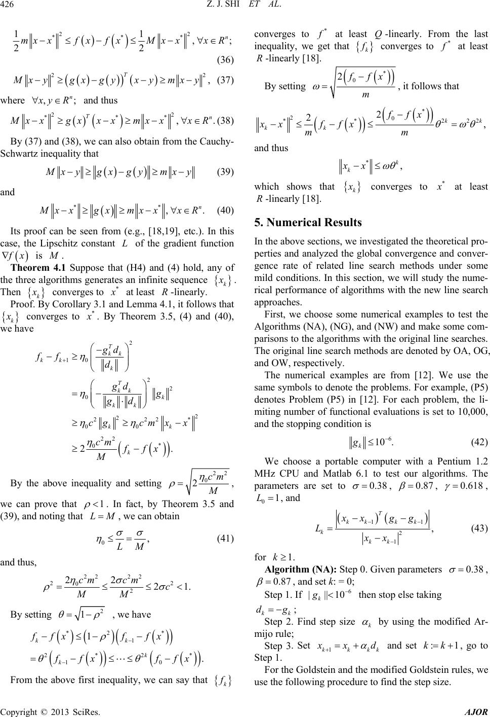

Z. J. SHI ET AL. 426


22
***
11
,;
22
converges to *
f
at least -linearly. From the last
inequality, we g thatQ et


k
f
n
x R mxxf xfxMxx 
(36
converges to *
f
)
   
2,
T2
M
xygx gyxymxy
at least
-linearly [18 R].
By setting



(37)
,;
n
x
yR where and thus


22
***
,.
n
T
M
xx xxx gmxxxR (38)
By (37) and (38), we can also obtain from the Cau
Schwartz inequality that chy-
 
M
xygxgymxy  (39)
and

**
,.
n
M
xxgxmxxxR  (40)
Its proof can be seen from (e.g., [18,19], etc.).
case, the Lipschitz constant of the gradient function
In this
L

f
x is 
M
.
Theorem 4.1 Suppose thaH4) and (4) hold, any of
e algtht ( the threorims generates an infinite sequen ce


k
x
.
Then

k
x
converges to *
x
at least R-linearly.
Proof. By Corollary 3.1 and Lemma 4.1, it follow

k
s that
x
erges to * conv
x
. By Theorem 35, (4) and .(40),
we have


2
T
kk
f10
2
2
0
2
2
22 2*
00
22 *
0
2.
kk
k
T
kk k
kk
kk
k
gd
fd
gd g
gd
cgcmx x
cm ffx
M

















 

By the above inequality and setting 22
0
2cm
M

 ,
we can prove that 1

. In fact, by Td heorem 3.5 an
(39), and noting th, we can obtain at LM
0,
LM


   (41)
and thus,
22 22
22
02
2221 cm cm c.
M
M

  
By setting 2 1

  , we have
*
From the above first inequality, we can say that
 

   
* *
2*2
10
1
.
k
k
x
ffxffx





 

2
1kk
fff fx

 


k
f
*
0
2
f
fx
m


, it follows that





*
2
*2
2ffx
x f0
*222
,
kk
xf
mm
kk
x

 
an


d thus
*
xx ,
k
k


which shows

that


k
x
*
x
converges to at least
5. Numerical Results
we iretical
ehe gl
geted line search methods r some
ion, we will studnume-
hms with the nerch
tively.
ion is
R-linearly [18].
a
ec
In the above section s, nvestigated the theopro-
prties and analyzed tobal convergenced conver-
nce rate of rel an unde
y the
w line sea
mild conditions. In this sect
rical performance of algorit
approaches.
First, we choose some numerical examples to test the
Alg ori thms ( NA) , (NG) , and ( NW) an d mak e some com-
parisons to the algorith ms with the original line searches.
The original line search methods are denoted by OA, OG,
and OW, resp
The numerical examples are from [12]. We use the
same symbols to denote the problems. For example, (P5)
denotes Problem (P5) in [12]. For each problem, the li-
miting number of functional evaluations is set to 10,000,
and the stopping condit
6
10 .
k
g  (42)
We choose a portable computer with a Pentium 1.2
MHz CPU and Matlab 6.1 to test our algorithms. The
parameters are set to 0.38


, 0.87

, 0.618


,
01L

, and
 
11
2
1
,
T
kkk k
k
xx gg
Lxx



 (43)
1.
kk
forAlgorithm : Step 0. Given paramete k (NA)rs 0.38


,
0.87


, and : = 0;
Step 1. If set k ||
k
g6 |10

 then stop else takin
k
g
k
dg

;
S Ftep 2.ind step size k

by using the modi-
ijo rule;
. Set
fied Ar
mStep 3kk1kk
x
xd



 and set :1kk
ep 1. , go to StFor the Goldstein and the modified Goldstein rules, we
use e the following procedurto find the step size.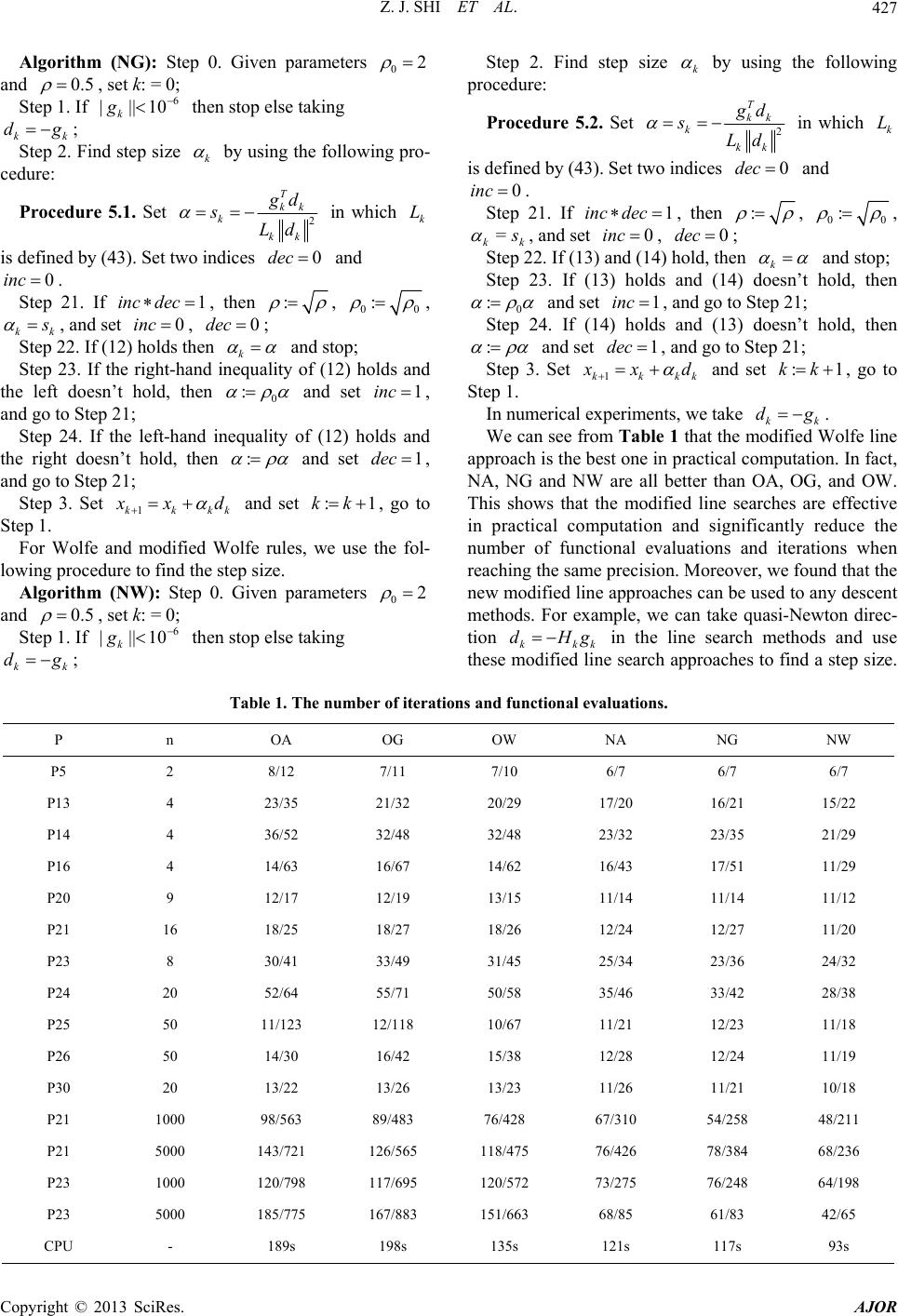

Z. J. SHI ET AL. 427
m (NG): Step 0. Given parameters Algorith 02


and 0.5

, s
Step 1et k: = 0; . If then stop else taking
6
|||10
k
g 
kk
g ;
Step 2. Find step size k
d

by using the following pro-
ce
5.1. Set
dure:
Procedure 2
kk
k
T
kk
g
dich
is
Step 21. If , then
sLd
  in wh k L
defined by (43). Set two indices 0dec and
0inc . 1inc dec :

 , 00 :

,
kk
s

, and set 0inc , 0dec

;
Step 22. If (12) holds thenk


lit
 and stop;
y of lds and
the lefoesn’t hold, then
Step 23. If the right-hand inequa(12) ho
t d 0 :

  and set 1inc

,
an1;
Step left-ha inequay of (12) holds and
th
d go to Step 2
24. If thendlit
e right doesn’t hold, then :

   and set 1dec

,
and go to Step 21;
Step 3. Set 1kkkk
x
xd

 t :1kk o
Step 1. and se go t
p size.
): Step 0. Given parameters
,
For Wolfe and modified Wolfe rules, we use the fol-
lowing procedure to find the ste
Algorithm (NW 02


and 0.5

, s
Step 1et k: = 0; . If then stop else taking
ind step sStep 2. Fize k

by using the following
procedure:
6
|||10
k
g 
kk
g ; d
Procedure 5.2. Set 2
T
kk
k
kk
g
d
  in which sLd
iso indices
k
L
defined by (43). Set tw and 0dec
0inc

.
Step 21. If 1inc dec

, then :

 , 0 :0

,
ks=

, and
kset 0inc

,
3) and (14) h0dec; Step 22. If (1old, then k


23. If (1s 4) doe sn’t and stop; Step 3) holdand (1 hold, then
0
:



and set 1inc

, and go to S tep 21;
Step 24. If (14) holds and (13) doesn’t hold, then
:



and set dec , an d go to Step 2 1 ; 1

Step 3. Set 1kkkk
x
xd



 and set :1kk , go to
Step 1. experiments, w
n see from Table 1 that the mWolfe line
ap mputation. In fact,
N
In numericale take kk dg
We ca. odified
proach is the best one in practical co
A, NG and NW are all better than OA, OG, and OW.
This shows that the modified line searches are effective
in practical computation and significantly reduce the
number of functional evaluations and iterations when
reaching the same precision. Moreover, we found that the
new modified line approaches can be used to any descent
methods. For example, we can take quasi-Newton direc-
tion kkk
dHg

 in the line search methods and use
these modified line search approaches to find a step size.
s and functional evaluations.
Table 1. The numberat
n
of iterion
P OA OG OW NA NG NW
P5 2 6/7 6/7 8/12 7/11 7/10 6/7
P13
2 23/35 21/29
1
5 1 1 1
CPU - 189s 198s 135s 121s 117s 93s
4 23/35 21/32 20/29 17/20 16/21 15/22
P14 4 36/52 32/48 32/48 3/32
P16 4 14/63 16/67 14/62 16/43 17/51 11/29
P20 9 12/17 12/19 13/15 11/14 11/14 11/12
P21 16 18/25 18/27 18/26 12/24 12/27 11/20
P23 8 30/41 33/49 31/45 25/34 23/36 24/32
P24 20 52/64 55/71 50/58 35/46 33/42 28/38
P25 50 11/123 12/118 10/67 11/21 12/23 11/18
P26 50 14/30 16/42 15/38 12/28 12/24 11/19
P30 20 13/22 13/26 13/23 11/26 11/21 10/18
P21 00098/563 89/483 76/428 67/310 54/258 48/211
P21 00043/72126/56518/47576/426 78/384 68/236
P23 1000 120/798 117/695 120/572 73/275 76/248 64/198
P23 5000 185/775 167/883 151/663 68/85 61/83 42/65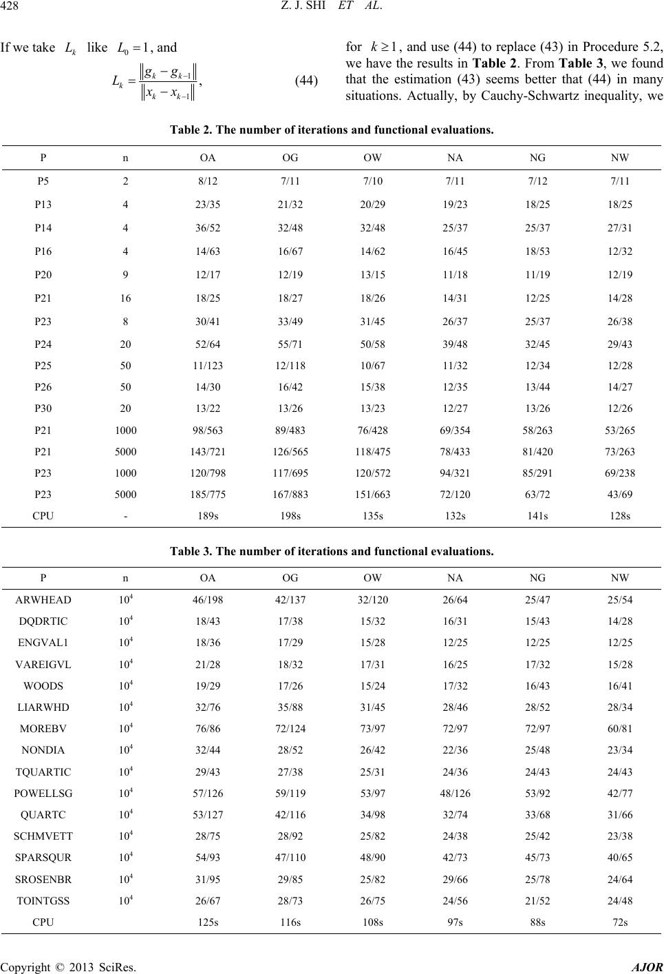

Z. J. SHI ET AL. 428
If we like , and
take k
L0 L1
1
1
,
kk
kkk
gg
xx



 )
f, and u to repla) in Pro5.2,
we he results inTable 2. F Table 3, wound
thstimatio) seems that (44) in many
sits. Actua Cauchyneq, we
2. The number of iteration
P n O
L (44
or 1kse (44)ce (43cedure
ave th
at the e n (43rom better e f
uationlly, by-Schwartz iuality
Table s and functional evaluations.
OW NA NG NW A OG
P5 2 8/12 7/11 7/10 7/11 7/12 7/11
P13 4 18/25 18/25
P14
1
5
1 1 1
1 1 1 1
23/35 21/32 20/29 19/23
4 36/52 32/48 32/48 25/37 25/37 27/31
P16 4 14/63 16/67 14/62 16/45 18/53 12/32
P20 9 12/17 12/19 13/15 11/18 11/19 12/19
P21 16 18/25 18/27 18/26 14/31 12/25 14/28
P23 8 30/41 33/49 31/45 26/37 25/37 26/38
P24 20 52/64 55/71 50/58 39/48 32/45 29/43
P25 50 11/123 12/118 10/67 11/32 12/34 12/28
P26 50 14/30 16/42 15/38 12/35 13/44 14/27
P30 20 13/22 13/26 13/23 12/27 13/26 12/26
P21 00098/563 89/483 76/428 69/354 58/263 53/265
P21 00043/72126/56518/47578/433 81/420 73/263
P23 00020/79817/69520/57294/321 85/291 69/238
P23 5000 185/775 167/883 151/663 72/120 63/72 43/69
CPU - 189s 198s 135s 132s 141s 128s
Tabe numbations and functional ens. le 3. Ther of itervaluatio
P n OA OG OW NA NG NW
ARWHEAD 10 46/198 42/137 32/120 26/64 25/47 25/54
4
DQDRTIC 104 15/43 14/28
ENGL1
P
33/68
S
CPU 125s 116s 108s 97s 88s 72s
18/43 17/38 15/32 16/31
VA 10418/36 17/29 15/28 12/25 12/25 12/25
VAREIGVL 104 21/28 18/32 17/31 16/25 17/32 15/28
WOODS 104 19/29 17/26 15/24 17/32 16/43 16/41
LIARWHD 104 32/76 35/88 31/45 28/46 28/52 28/34
MOREBV 104 76/86 72/124 73/97 72/97 72/97 60/81
NONDIA 104 32/44 28/52 26/42 22/36 25/48 23/34
TQUARTIC 104 29/43 27/38 25/31 24/36 24/43 24/43
OWELLSG 104 57/126 59/119 53/97 48/126 53/92 42/77
QUARTC 104 53/127 42/116 34/98 32/74 31/66
SCHMVETT 104 28/75 28/92 25/82 24/38 25/42 23/38
SPARSQUR 104 54/93 47/110 48/90 42/73 45/73 40/65
ROSENBR 104 31/95 29/85 25/82 29/66 25/78 24/64
TOINTGSS 104 26/67 28/73 26/75 24/56 21/52 24/48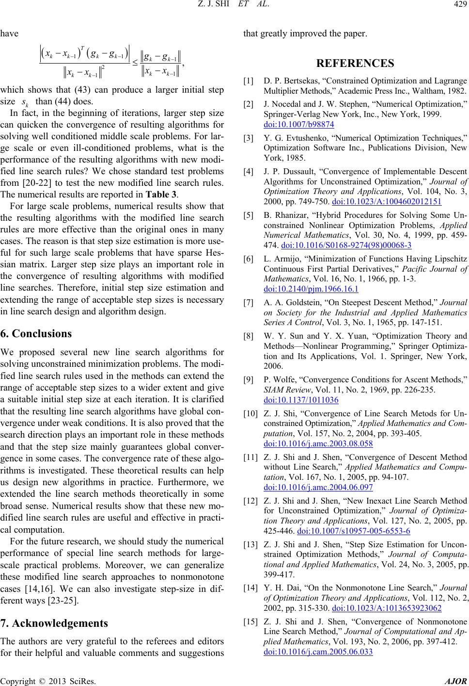

Z. J. SHI ET AL. 429
have
 
11 1
21
1
,
T
kkk kkk
kk
kk
xx gg
x
xx
 





hows that (43) can produce a larger initial step
gg
x
which s
size k
s
than (44) does.
In, in the beginning of iterations, larger step size
can quicken the convergence of resulting algoms for
solving well conditioned middle scale problems. For lar-
m
an extend the
to a wider extent and
p size at each iteration. It is clarified
that greatly improved the paper.
ERENCES
[1] P. Bertsekaonstrained ization andrange
s,” Academic Press Inc., Waltham, 1982.
. Stephen, “Numerical Optimization,”
, Inc., New York, 1999.
factrith
ge scale or even ill-conditioned problems, what is the
perforance of the resulting algorithms with new modi-
fied line search rules? We chose standard test problems
from [20-22] to test the new modified line search rules.
The numerical results are reported in Table 3.
For large scale problems, numerical results show that
the resulting algorithms with the modified line search
rules are more effective than the original ones in many
cases. The reason is that step size estimation is more use-
ful for such large scale problems that have sparse Hes-
sian matrix. Larger step size plays an important role in
the convergence of resulting algorithms with modified
line searches. Therefore, initial step size estimation and
extending the range of acceptable step sizes is necessary
in line search design and algorith m design .
6. Conclusions
We proposed several new line search algorithms for
solving unconstrained minimization problems. The modi-
fied line search rules used in the methods c
range of acceptable step sizes
a suitable initial stegive
that the resulting line search algorith ms have global con-
vergence und er weak con d itions . It is also pro ved th at th e
search direction plays an important role in these methods
and that the step size mainly guarantees global conver-
gence in some cases. The convergence rate of these algo-
rithms is investigated. These theoretical results can help
us design new algorithms in practice. Furthermore, we
extended the line search methods theoretically in some
broad sense. Numerical results show that these new mo-
dified line search rules are useful and effective in practi-
cal computation.
For the future research, we should study the numerical
performance of special line search methods for large-
scale practical problems. Moreover, we can generalize
these modified line search approaches to nonmonotone
cases [14,16]. We can also investigate step-size in dif-
ferent ways [23-25].
7. Acknowledgements
The authors are very grateful to the referees and editors
for their helpful and valuable comments and suggestions
Multiplier Method
[2] J. Nocedal and J. W
REF
D. s, “COptim Lag
Springer-Verlag New York
doi:10.1007/b98874
[3] Y. G. Evtushenko, “Numerical Optimization Techniques,”
Optimization Software Inc., Publications Division, New
York, 1985.
[4] J. P. Dussault, “Convergence of Implementable Descent
Algorithms for Unconstrainedization,” Journal of
Optimization , Vol. 104, No. 3,
Optim
Theory and Applications
2000, pp. 749-750. doi:10.1023/A:1004602012151
[5] B. Rhanizar, “Hybrid Procedures for Solving Some Un-
constrained Nonlinear Optimization Problems, Applied
Numerical Mathematics, Vol. 30, No. 4, 1999, pp. 459-
474. doi:10.1016/S0168-9274(98)00068-3
[6] L. Armijo, “Minimization of Functions Having Lipschitz
Continuous First Partial Derivatives,” Pacific Journal of
Mathematics, Vol. 16, No. 1, 1966, pp. 1-3.
doi:10.2140/pjm.1966.16.1
[7] A. A. Goldstein, “On Steepest Descent Method,” Journal
on Society for the Industrial and Applied Mathematics
Series A Control, Vol. 3, No. 1, 1965, pp. 147-151.
[8] W. Y. Sun and Y. X. Yuan, “Optimization Theory and
Methods—Nonlinear Programming,” Springer Optimiza-
tion and Its Applications, Vol. 1. Springer, New York,
2006.
[9] P. Wolfe, “Convergence Conditions for Ascent Methods,”
SIAM Review, Vol. 11, No. 2, 1969, pp. 226-235.
doi:10.1137/1011036
[10] Z. J. Shi, “Convergence of Line Search Metods for Un-
constrained Optimization,” Applied Mathematic s and Com-
putation, Vol. 157, No. 2, 2004, pp. 393-405.
doi:10.1016/j.amc.2003.08.058
[11] Z. J. Shi and J. Shen, “Convergence of Descent Method
without Line Search,” Applied Mathematics and Compu-
tation, Vol. 167, No. 1, 2005, pp. 94-107.
doi:10.1016/j.amc.2004.06.097
[12] Z. J. Shi and J. Shen, “New Inexact Line Search Method
for Unconstrained Optimization,” Journal of Optimiza-
tion Theory and Applications, Vol. 127, No. 2, 200
425-446. 5, pp. 10957-005-6553-6doi:10.1007/s
, 2005, pp.
23062
[13] Z. J. Shi and J. Shen, “Step Size Estimation for Uncon-
strained Optimization Methods,” Journal of Computa-
tional and Applied Mathematics, Vol. 24, No. 3
399-417.
[14] Y. H. Dai, “On the Nonmonotone Line Search,” Journal
of Optimization Theory and Applications, Vol. 112, No. 2,
2002, pp. 315-330. doi:10.1023/A:10136539
[15] Z. J. Shi and J. Shen, “Convergence of Nonmonotone
Line Search Method,” Journal of Computational and Ap-
plied Mathematics, Vol. 193, No. 2, 2006, pp. 397-412.
doi:10.1016/j.cam.2005.06.033

Z. J. SHI ET AL. 430
[16] W. Y. Sun, J. Y. Han and J. Sun, “Global Convergence of
Nonmonotone Descent Methods for Unconstrained Opti-
mization Problems,” Journal of Computational and Ap-
plied Mathematics, Vol. 146, No. 1, 2002, pp. 89-98.
doi:10.1016/S0377-0427(02)00420-X
[17] H. C. Zhang and W. W. Hager, “A Nonmonotone Line
Search Technique and Its Application to Unconstrained
Optimization,” The SIAM Journal on Optimization, Vol.
14, No. 4, 2004, pp. 1043-1056.
doi:10.1137/S1052623403428208
[18] J. M. Ortega and W. C. Rheinboldt, “Iterative Solution of
Nonlinear Equations in Several Variables,” Academic
Press, Walth am , 1970.
[19] R. T. Rockafellar, “Convex Analysis,” Princeton Univer-
sity Press, Princeton, 1970.
[20] I. Bongartz, A. R. Conn, N. I. M. Gould and P. L. Toi
“CUTE: Constrained and Unconstrai nt ned Testing Envi-
,
ronments,” ACM Transactions on Mathematical Software,
Vol. 21, No. 1, 1995, pp. 123-160.
doi:10.1145/200979.201043
[21] W. W. Hager and H. C. Zhang, “A New Conjugate Gra-
dient Method with Guaranteed Descent and an Efficient
Line Search,” The SIAM Journal on Optimization, Vol.
16, No. 1, 2005, pp. 170-192. doi:10.1137/030601880
[22] W. W. Hager and H. C. Zhang, “
DESCENT, A Conjugate Gradient Method
Algorithm 851: CG
with Guaran-
teed Descent,” ACM Transactions on Mathematical Soft-
ware, Vol. 32, No. 1, 2006, pp. 113-137.
doi:10.1145/1132973.1132979
[23] A. I. Cohen, “Stepsize Analysis for Descent Methods,”
Journal of Optimization Theory and Applications, Vol. 33,
No. 2, 1981, pp. 187-205. doi:10.1007/BF00935546
[24] J. C. Gilbert and J. Nocedal, “Global Convergence Pro-
perties of Conjugate Gradie nt Methods for
The SIAM Journal on OptimizaOptimization,” tion, Vol. 2, No. 1, 1992,
pp. 21-42. doi:10.1137/0802003
[25] Z. J. Shi, “A New Memory Gradient Method under Exact
Line Search,” Asia-Pacific Journal of Operational Re-
search, Vol. 20, No. 2, 2003, pp. 275-284.