J. Serv. Sci. & Management. 2008, 1: 21-27
Published Online June 2008 in SciRes (www.SRPublishing.org/journal/jssm)
Research on Supply Chain Inventory Optimization and
Benefit Coordination with Controllable Lead Time
Fei Ye，Yi-Na Li，Xue-Jun Xu and Jian-Hui Zhao
School of Business Administration, South China University of Technology, Guangzhou, P.R.China 510640
ABSTRACT
In this paper, we propose two supply chain inventory models with controllable lead time, the first is proposed under
centralized decision mode and the other is proposed under decentralized decision mode. The solution procedures are
also suggested to get the optimal solutions. In addition, taking individual rationality into consideration, Shapely value
method and MCRS method are used to coordinate th e benefits of the vendo r and the buyer. Numerical example is given
to illustrate the results of the propo sed models.
Keywords: Supply Chain Inventory Model, Controllable Lead Time, Shapely Value, MCRS Method
1. Introduction
Time-based competition (TBC) has been one of the most
popular competitive modes and time management is be-
coming more and more important in this increasing in-
tense competitive environment [1]. In most of traditional
economic order quantity literatures, lead time is viewed
as a constant or a stochastic variable by either using de-
terministic or probabilistic models, that is, lead time is
assumed to be not subject to control [2,3]. However, this
may not be realistic. As pointed out by Tersine [4], lead
time usually is consisted of five components: order
preparation time, order transmit time, vendor’s lead time,
delivery time and setup time. In many practical cases,
lead time can be reduced by an added crashing cost, that
is, it is controllable. The benefit of reducing lead time,
such as lower safety stock, decrease stock out loss, en-
hance customer service level, and obtain the competitive
advantages has been clearly evidenced by successful ex-
perience of using Just-In-Time (JIT) production. Lead
time reduction has been viewed to be an effective way to
realize the quick response of the whole supply chain and
one of the most important sources of competitive advan-
tage [1].
Liao & Shyu (1991) [5] first put forward a continuous
review model where order quantity is predetermined and
lead time is the only decision variable. Ben-Daya &
Raouf (1994 ) [6] extended Liao & Shyu’s model (1991)
by viewing both lead time and order quantity as decision
variables. Ouyang et al. (1996) [7] further took the as-
sumption that the shortage could be divided into a mix-
ture of backord ers and lost sales. Ouyang&Wu (199 8) [8]
viewed that the demand of lead time can be any known
and free cumulative distribution, and proposed procedures
to get the optimal lead time and order quantity under dif-
ferent situations. Moon&Choi (1998) [9] extended Ouy-
ang et al.’s model (1996) by consid ering the reorder poin t
to be another decision variable. Ouyang&Chang (2000)
[10] improved Ouyang et al.’s model (1996 ) by further
assuming the backorder rate is not a determined constant,
but be dependent on the length of lead time. All of these
above models only took the optimal policy decisions for
the buyer into consider ation. However, the growing focus
on supply chain management for this increasing intense
competitive environment calls for a more efficient man-
agement of inventories across the whole supply chain
through more coordination and cooperation. In recent
paper, Pan & Yang (2002) [11] extended Goyal’s model
(1988) [12] by assuming lead time as a controllable vari-
able and gained a lower joint expected cost and shorter
lead time of the entire supply chain compared to that of
Goyal’s model. Ouyang et al. (2004) [13] improved Pan
& Yang’s model (2002) by further assuming the reorder
point as the other decision variable and shortages is per-
mitted, optimizing ordering quantity, lead time, reorder
point and the number of lots simultaneously in an inte-
grated supply chain inventory model.
In this paper, we consider the single vendor single
buyer inventory p roblem. As known to all, a supply chain
can be viewed as a network which is consisted of series of
suppliers, manufacturers, retailers, and customers,
through the physical flow, information flow and financial
flow. It is beginning with the raw materials producing by
a supplier and ending with the product consumption by
customers. A node in the supply chain network represents
a physical site, a sub-network, or an operation process,
and links represent physical flow. However, all supply
chain network (SCN) can be divided into several
one-to-one supply models consists of single vendor and
single buyer under certain conditions. This kind of
one-to-one supply model is the basis of supply chain
network analysis. Hence, we only take the two-echelon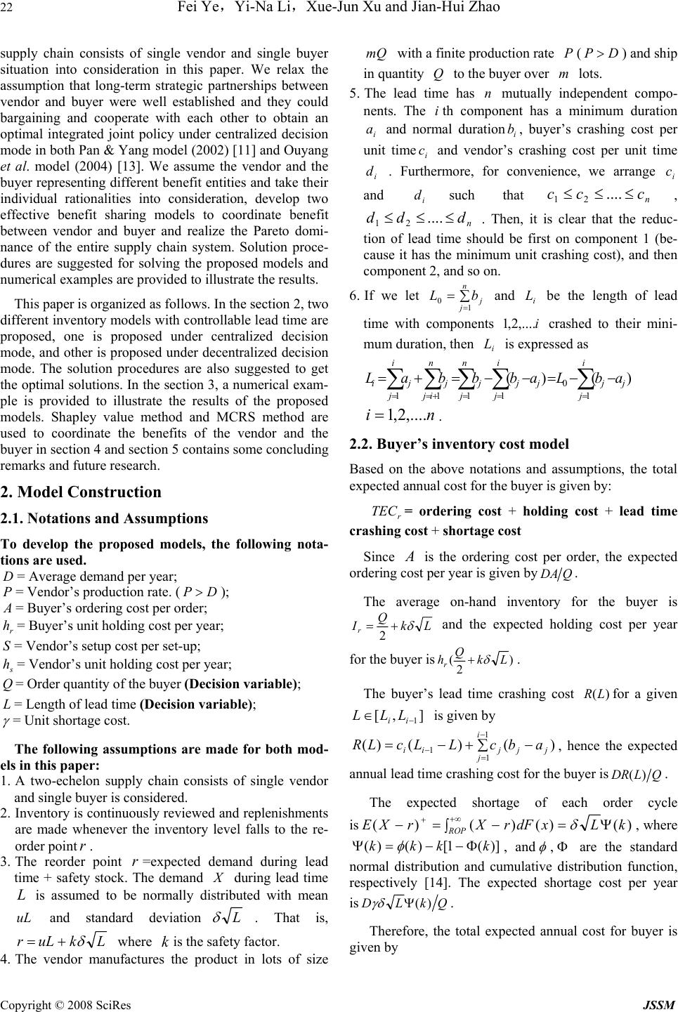

22 Fei Ye，Yi-Na Li，Xue-Jun Xu and Jian-Hui Zhao
supply chain consists of single vendor and single buyer
situation into consideration in this paper. We relax the
assumption that long-term strategic partnerships between
vendor and buyer were well established and they could
bargaining and cooperate with each other to obtain an
optimal integrated joint policy under centralized decision
mode in both Pan & Yang model (2002) [11] and Ouyang
et al. model (2004) [13]. We assume the vendor and the
buyer representing differen t benefit entities and take their
individual rationalities into consideration, develop two
effective benefit sharing models to coordinate benefit
between vendor and buyer and realize the Pareto domi-
nance of the entire supply chain system. Solution proce-
dures are suggested for solving the proposed models and
numerical examples are provided to illustrate the results.
This paper is organized as follows. In th e section 2, two
different inventory models with controllable lead time are
proposed, one is proposed under centralized decision
mode, and other is proposed under decentralized decision
mode. The solution procedures are also suggested to get
the optimal solutions. In the section 3, a numerical exam-
ple is provided to illustrate the results of the proposed
models. Shapley value method and MCRS method are
used to coordinate the benefits of the vendor and the
buyer in section 4 and section 5 contains some concluding
remarks an d f u t ur e r es ear ch.
2. Model Construction
2.1. Notations and Assumptions
To develop the proposed models, the following nota-
tions are used.
D= Average demand per year;
P
= Vendor’s production rate. (D
P
>);
A
= Buyer’s ordering cost per order;
r
h= Buyer’s unit hol din g c ost per year;
S= Vendor’s setup cost per set-up;
s
h= Vendor’s unit holding cost per year;
Q= Order quantity of the buyer (Decision variable);
L= Length of lead time (Decision variable);
γ
= Unit shortage cost.
The following assumptions are made for both mod-
els in this paper:
1. A two-echelon supply chain consists of single vendor
and single buyer is consider ed.
2. Inventory is continuously reviewed and replenishments
are made whenever the inventory level falls to the re-
order point
r
.
3. The reorder point
r
=expected demand during lead
time + safety stock. The demand
X
during lead time
L is assumed to be normally distributed with mean
uL and standard deviationL
δ
. That is,
LkuLr δ += where kis the safety factor.
4. The vendor manufactures the product in lots of size
mQ with a finite production rate
P
(D
P
>) and ship
in quantity Q to the buyer over m lots.
5. The lead time has n mutually independent compo-
nents. The ith component has a minimum duration
i
a and normal durationi b, buyer’s crashing cost per
unit timei c and vendor’s crashing cost per unit time
i
d . Furthermore, for convenience, we arrange i c
and i
dsuch thatn
ccc
≤
≤≤ ....
21 ,
n
ddd
≤
≤
≤
....
21 . Then, it is clear that the reduc-
tion of lead time should be first on component 1 (be-
cause it has the minimum unit crashing cost), and then
component 2, and so on.
6. If we let ∑
==
n
jj
bL 1
0 and i
L be the length of lead
time with components i,....2,1 crashed to their mini-
mum duration, then i L is expressed as
∑∑∑∑∑ ====+=
−−=−−=+= i
jjj
i
jjj
n
jj
i
j
n
ijjji abLabbbaL
1
0
1111
)()(
ni ,....2,1
=
.
2.2. Buyer’s inventory cost model
Based on the above notations and assumptions, the total
expected annual cost for the buyer is given by:
r
TEC = ordering cost + holding cost + lead time
crashing cost + shortage cost
Since A is the ordering cost per order, the expected
ordering cost per year is given byQDA .
The average on-hand inventory for the buyer is
Lk
Q
Ir δ += 2 and the expected holding cost per year
for the buyer is)
2
(Lk
Q
hr δ +.
The buyer’s lead time crashing cost )(LR for a given
],[1−
∈
ii LLL is given by
∑−+−= −
=
−
1
1
1)()()( i
jjjjii abcLLcLR , hence the expected
annual lead time crashing cost for the buyer isQLDR )( .
The expected shortage of each order cycle
is )()()()( kLxdFrXrXE ROP Ψ=
∫−=− +∞
+
δ , where
)](1[)()( kkkk
Φ
−
−
=
Ψ
φ
, and
φ
,Φ are the standard
normal distribution and cumulative distribution function,
respectively [14]. The expected shortage cost per year
is QkLD )(Ψ γδ
.
Therefore, the total expected annual cost for buyer is
given by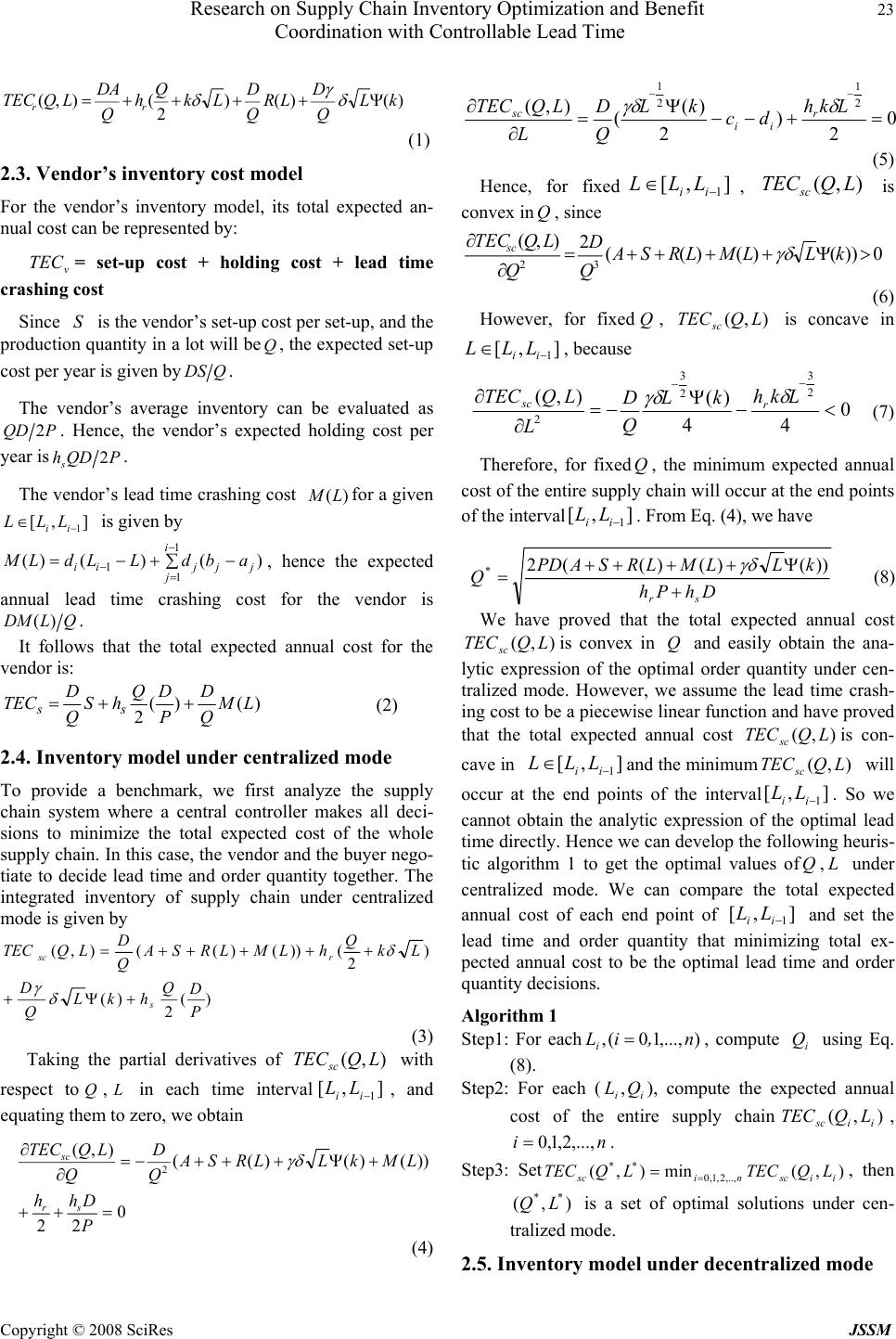

Research on Supply Chain Inventory Optimization and Benefit 23
Coordination with Controllable Lead Time
)()()
2
(),(kL
Q
D
LR
Q
D
Lk
Q
h
Q
DA
LQTEC rr Ψ++++= δ
γ
δ
(1)
2.3. Vendor’s inventory cost model
For the vendor’s inventory model, its total expected an-
nual cost can be represented by:
v
TEC = set-up cost + holding cost + lead time
crashing cost
Since S is the vendor’s set-up cost per set-up, and the
production quan tity in a lot will beQ, the expected set-up
cost per year is given byQDS .
The vendor’s average inventory can be evaluated as
PQD 2. Hence, the vendor’s expected holding cost per
year isPQDhs2.
The vendor’s lead time crashing cost )(LM fo r a given
],[1− ∈ii LLL is g iven by
∑−+−=−
=
−
1
1
1)()()(i
jjjjii abdLLdLM, hence the expected
annual lead time crashing cost for the vendor is
QLDM )( .
It follows that the total expected annual cost for the
vendor is:
)()(
2LM Q
D
P
DQ
hS
Q
D
TEC ss ++= (2)
2.4. Inventory model under centralized mode
To provide a benchmark, we first analyze the supply
chain system where a central controller makes all deci-
sions to minimize the total expected cost of the whole
supply chain. In this case, the vendor an d the buyer nego-
tiate to decide lead time and order quantity together. The
integrated inventory of supply chain under centralized
mode is given by
)(
2
)(
)
2
())()((),(
P
D
Q
hkL
Q
D
Lk
Q
hLMLRSA
Q
D
LQTEC
s
rsc
+Ψ+
+++++=
δ
γ
δ
(3)
Taking the partial derivatives of ),( LQTECsc with
respect toQ,
L
in each time interval],[ 1−ii LL , and
equating them to zero, we obtain
0
22
))()()((
),(
2
=++
+Ψ+++−=
∂
∂
P
Dhh
LMkLLRSA
Q
D
Q
LQTEC
sr
sc
γδ
(4)
0
2
)
2
)(
(
),( 2
1
2
1
=+−−
Ψ
=
∂
∂−
−Lkh
dc
kL
Q
D
L
LQTECr
ii
sc
δ
γδ
(5)
Hence, for fixed],[ 1−
∈
ii LLL , ),( LQTECsc is
convex inQ, since
0))()()((
2
),(
32 >Ψ++++=
∂
∂kLLMLRSA
Q
D
Q
LQTECsc
γδ
(6)
However, for fixedQ, ),( LQTECsc is concave in
],[ 1−
∈
ii LLL , because
0
44
)( ),( 2
3
2
3
2<−
Ψ
−=
∂
∂−
−Lkh
kL
Q
D
L
LQTEC r
sc
δ γδ
(7)
Therefore, for fixed Q, the minimum expected annual
cost of the entire supply chain will occur at the end po ints
of the interval],[ 1−ii LL . F rom Eq. (4), we have
DhPh
kLLMLRSAPD
Q
sr +
Ψ++++
=))()()((2
*
γδ
(8)
We have proved that the total expected annual cost
),( LQTECsc is convex in Q and easily obtain the ana-
lytic expression of the optimal order quantity under cen-
tralized mode. However, we assume the lead time crash-
ing cost to be a piecewise linear function and have proved
that the total expected annual cost ),( LQTECsc is con-
cave in ],[ 1−
∈
ii LLL an d t he min i mu m),( LQTECsc will
occur at the end points of the interval],[ 1−ii LL . So we
cannot obtain the analytic expression of the optimal lead
time directly. Hence we can develop the following heuris-
tic algorithm 1 to get the optimal values of Q,L under
centralized mode. We can compare the total expected
annual cost of each end point of ],[ 1−ii LL and set the
lead time and order quantity that minimizing total ex-
pected annual cost to be the optimal lead time and order
quantity decisions.
Algorithm 1
Step1: For each),...,10(, n
， iLi
=
, compute i Q using Eq.
(8).
Step2: For each (ii QL ,), compute the expected annual
cost of the entire supply chain),( iisc LQTEC ,
ni ,...,2,1,0
=
.
Step3: Set),(min),( ,..,2,1,0
**iiscnisc LQTECLQTEC =
=, then
),( **LQ is a set of optimal solutions under cen-
tralized mode.
2.5. Inventory model under decentralized mode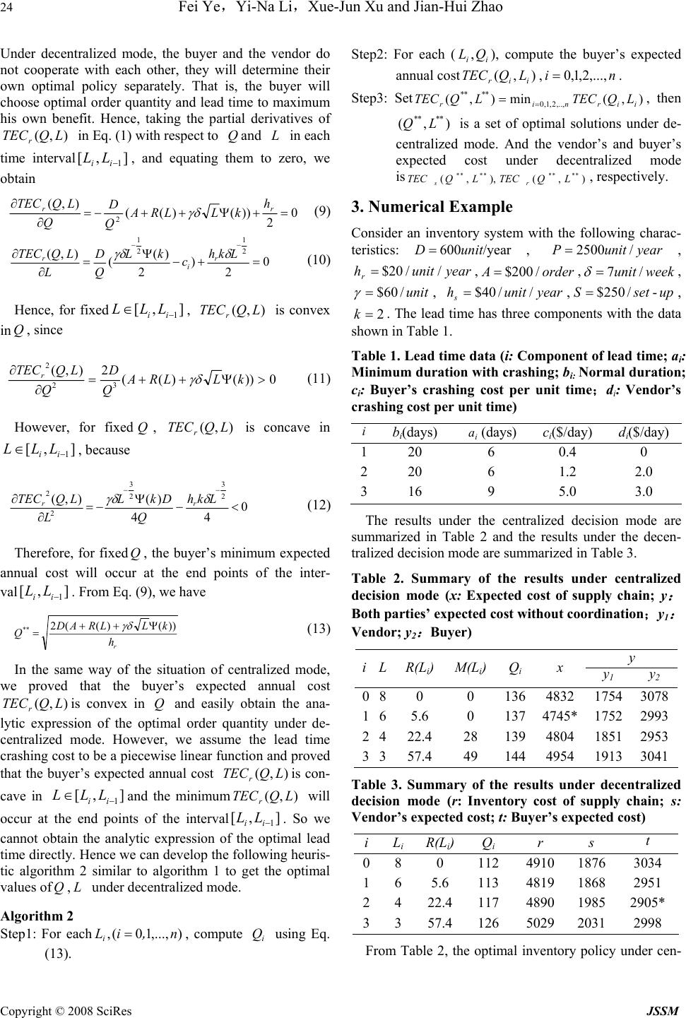

24 Fei Ye，Yi-Na Li，Xue-Jun Xu and Jian-Hui Zhao
Under decentralized mode, the buyer and the vendor do
not cooperate with each other, they will determine their
own optimal policy separately. That is, the buyer will
choose optimal order qu antity and lead time to maximum
his own benefit. Hence, taking the partial derivatives of
),( LQTECr in Eq. (1) with resp ect to Qand L in each
time interval],[ 1−ii LL , and equating them to zero, we
obtain
0
2
))()((
),(
2=+Ψ++−=
∂
∂rr h
kLLRA
Q
D
Q
LQTEC
γδ
(9)
0
2
)
2
)(
(
),( 2
1
2
1
=+−
Ψ
=
∂
∂−− Lkh
c
kL
Q
D
L
LQTEC r
i
r
δγδ
(10)
Hence, for fixed],[ 1−
∈ii LLL , ),( LQTECr is convex
inQ, since
0))()((
2),(
32
2
>Ψ++=
∂
∂kLLRA
Q
D
Q
LQTECr
γδ
(11)
However, for fixedQ, ),( LQTECr is concave in
],[ 1− ∈ii LLL , because
0
44
)(),( 2
3
2
3
2
2
<−
Ψ
−=
∂
∂−− Lkh
Q
DkL
L
LQTEC rr δγδ
(12)
Therefore, for fixedQ, the buyer’s minimum expected
annual cost will occur at the end points of the inter-
val ],[ 1−ii LL . From Eq. (9), we have
r
h
kLLRAD
Q))()((2
** Ψ++
=
γδ
(13)
In the same way of the situation of centralized mode,
we proved that the buyer’s expected annual cost
),( LQTECris convex in Q and easily obtain the ana-
lytic expression of the optimal order quantity under de-
centralized mode. However, we assume the lead time
crashing cost to be a piecewise linear function and proved
that the buyer’s expected annual cost ),( LQTECris con-
cave in ],[ 1−
∈ii LLL and the minimum),( LQTECr will
occur at the end points of the interval],[ 1−ii LL . So we
cannot obtain the analytic expression of the optimal lead
time directly. Hence we can develop the following heuris-
tic algorithm 2 similar to algorithm 1 to get the optimal
values ofQ,L under decentralized mode.
Algorithm 2
Step1: For each),...,10(, n
， iLi=, compute i Q using Eq.
(13).
Step2: For each (ii QL,), compute the buyer’s expected
annual cost),( iir LQTEC,ni ,...,2,1,0=.
Step3: Set),(min),( ,..,2,1,0
**** iirnir LQTECLQTEC =
=, then
),( **** LQ is a set of optimal solutions under de-
centralized mode. And the vendor’s and buyer’s
expected cost under decentralized mode
is ),(),,(********LQTECLQTEC rs, respectively.
3. Numerical Example
Consider an inventory system with the following charac-
teristics: /year600unitD
=
, yearunitP /2500=,
yearunithr//20$
=
,orderA/200$
=
,weekunit /7=
δ
,
unit/60$
=
γ
, yearuniths//40$
=
,upsetS-/250$=,
2
=
k. The lead time has three components with the data
shown in Table 1.
Table 1. Lead time data (i: Component of lead time; ai:
Minimum duration with crashing; bi: Normal duration;
ci: Buyer’s crashing cost per unit time；di: Vendor’s
crashing cost per unit time)
ibi(days) i
a(days) ci($/day) di($/day)
120 6 0.4 0
220 6 1.2 2.0
316 9 5.0 3.0
The results under the centralized decision mode are
summarized in Table 2 and the results under the decen-
tralized decision mode are summarized in Table 3.
Table 2. Summary of the results under centralized
decision mode (x: Expected cost of supply chain; y
：
Both parties’ expected cost without coordination；y1 ：
Vendor; y2 ： Buyer)
y
iL R(L
i)M(Li)Q i x y1 y
2
080 0 136 4832 17543078
165.6 0 137 4745* 17522993
2422.4 28 139 4804 18512953
3357.4 49 144 4954 19133041
Table 3. Summary of the results under decentralized
decision mode (r: Inventory cost of supply chain; s:
Vendor’s expected cost; t: Buyer’s expe cted cost)
iL
i R(Li)Qi r s t
08 0 112 4910 1876 3034
16 5.6 113 4819 1868 2951
24 22.4117 4890 1985 2905*
33 57.4126 5029 2031 2998
From Table 2, the optimal inventory policy under cen-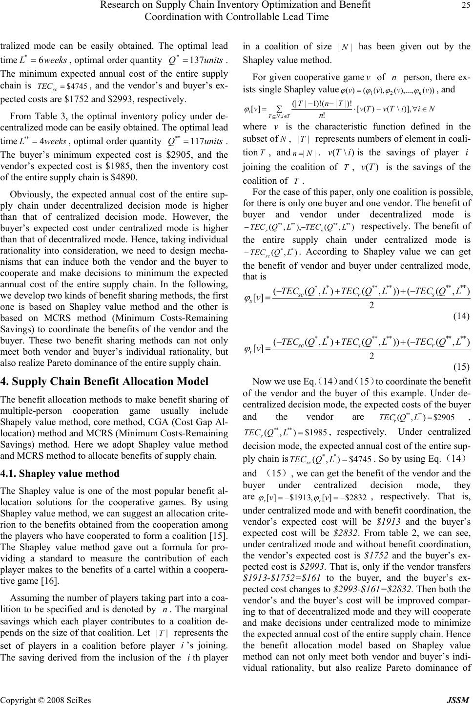

Research on Supply Chain Inventory Optimization and Benefit 25
Coordination with Controllable Lead Time
tralized mode can be easily obtained. The optimal lead
time weeksL 6
*=, optimal order quantity unitsQ 137 *=.
The minimum expected annual cost of the entire supply
chain is $4745=
sc
TEC , and the vendor’s and buyer’s ex-
pected costs are $1752 and $2993, respectively.
From Table 3, the optimal inventory policy under de-
centralized mode can be easily obtained. The optimal lead
time weeksL 4
** =, optimal order quantity unitsQ 117 ** =.
The buyer’s minimum expected cost is $2905, and the
vendor’s expected cost is $1985, then the inventory cost
of the entire supply chain is $4890.
Obviously, the expected annual cost of the entire sup-
ply chain under decentralized decision mode is higher
than that of centralized decision mode. However, the
buyer’s expected cost under centralized mode is higher
than that of decentralized mode. Hence, taking individual
rationality into consideration, we need to design mecha-
nisms that can induce both the vendor and the buyer to
cooperate and make decisions to minimum the expected
annual cost of the entire supply chain. In the following,
we develop two kinds of benefit sharing methods, the first
one is based on Shapley value method and the other is
based on MCRS method (Minimum Costs-Remaining
Savings) to coordinate the benefits of the vendor and the
buyer. These two benefit sharing methods can not only
meet both vendor and buyer’s individual rationality, but
also realize Pareto dominance of the entire supply chain.
4. Supply Chain Benefit Allocation Model
The benefit allocation methods to make benefit sharing of
multiple-person cooperation game usually include
Shapely value method, core method, CGA (Cost Gap Al-
location) method and MCRS (Minimum Costs-Remaining
Savings) method. Here we adopt Shapley value method
and MCRS method to allocate benefits of supply chain.
4.1. Shapley value method
The Shapley value is one of the most popular benefit al-
location solutions for the cooperative games. By using
Shapley value method, we can suggest an allocation crite-
rion to the benefits obtained from the cooperation among
the players who have cooperated to form a coalition [15].
The Shapley value method gave out a formula for pro-
viding a standard to measure the contribution of each
player makes to the benefits of a cartel within a coopera-
tive game [16].
Assuming the number of players taking part into a coa-
lition to be specified and is denoted by n. The marginal
savings which each player contributes to a coalition de-
pends on the size of that coalition. Let ||T represents the
set of players in a coalition before player i’s joining.
The saving derived from the inclusion of the ith player
in a coalition of size || N has been given out by the
Shapley value method.
For given cooperative game
v
of n person, there ex-
ists single Shapley value))(),...,(),(()( 21 vvvv n
ϕ
ϕ
ϕ
ϕ
=, and
NiiTvTv
n
TnT
vTiNT
i∈∀−⋅
∑−− =∈⊆ )],\()([
!
|)!|()!1|(|
][ , ϕ
where
v
is the characteristic function defined in the
subset ofN, ||T represents numbers of element in coali-
tion
T
, and|| Nn
=
. )\( iTv is the savings of player i
joining the coalition of
T
, )(Tv is the savings of the
coalition of
T
.
For the case of this paper, only one coalition is possible,
for there is only one buyer and one vendor. The benefit of
buyer and vendor under decentralized mode is
),(),,(******** LQTECLQTEC sr −− respectively. The benefit of
the entire supply chain under centralized mode is
),( ** LQTECsc −. According to Shapley value we can get
the benefit of vendor and buyer under centralized mode,
that is
2
),(()),(),((
][ ********** LQTECLQTECLQTEC vsrsc
s−++−
= ϕ
(14)
2
),(()),(),((
][ ********** LQTECLQTECLQTEC
vrssc
r−++−
=
ϕ
(15)
Now we use Eq. （14）and（15）to coordinate the benefit
of the vendor and the buyer of this example. Under de-
centralized decision mode, the expected costs of the buyer
and the vendor are2905$),( **** =LQTECr,
1985$),( **** =LQTECs, respectively. Under centralized
decision mode, the expected annual cost of the entire sup-
ply chain is4745$),( ** =LQTECsc . So by using Eq.（14）
and （15）, we can get the benefit of the vendor and the
buyer under centralized decision mode, they
are 2832$][,1913$][ −=−= vv rs ϕϕ , respectively. That is,
under centralized mode and with benefit coordination, the
vendor’s expected cost will be $1913 and the buyer’s
expected cost will be $2832. From table 2, we can see,
under centralized mode and without benefit coordination,
the vendor’s expected cost is $1752 and the buyer’s ex-
pected cost is $2993. That is, only if the vendor transfers
$1913-$1752=$ 161 to the buyer, and the buyer’s ex-
pected cost changes to $2993-$161=$2832. Then both the
vendor’s and the buyer’s cost will be improved compar-
ing to that of decentralized mode and they will cooperate
and make decisions under centralized mode to minimize
the expected annual cost of the entire supply chain. Hence
the benefit allocation model based on Shapley value
method can not only meet both vendor and buyer’s indi-
vidual rationality, but also realize Pareto dominance of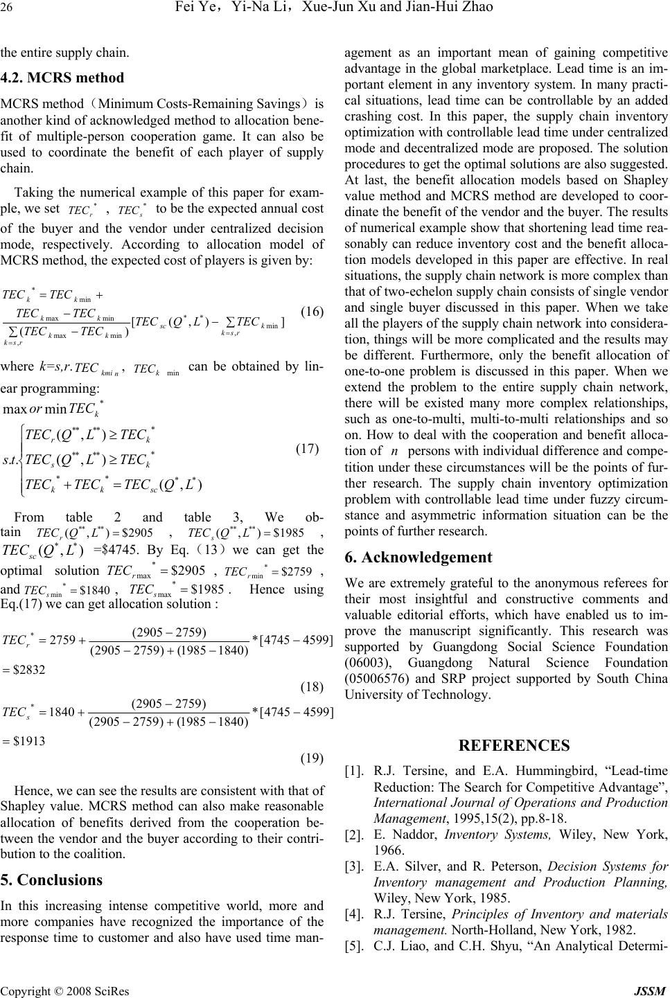

26 Fei Ye，Yi-Na Li，Xue-Jun Xu and Jian-Hui Zhao
the entire supply chain.
4.2. MCRS method
MCRS method （Minimum Costs-Remaining Savings） is
another kind of acknowledged method to allocation bene-
fit of multiple-person cooperation game. It can also be
used to coordinate the benefit of each player of supply
chain.
Taking the numerical example of this paper for exam-
ple, we set *
r
TEC , *
s
TEC to be the expected annual cost
of the buyer and the vendor under centralized decision
mode, respectively. According to allocation model of
MCRS method, the expected cost of players is give n by:
]),([
)( ,min
**
,minmax
minmax
min
*
∑
−
∑−
−
+=
=
=
rsk ksc
rsk kk
kk
kk
TECLQTEC
TECTEC
TECTEC
TECTEC (16)
where k=s,r.n
kmi
TEC , mink TEC can be obtained by lin-
ear programm ing:
⎪
⎪
⎩
⎪
⎪
⎨
⎧
=+
≥
≥
),(
),(
),(
..
minmax
**
**
*
****
*
****
*
LQTECTECTEC
TECLQTEC
TECLQTEC
ts
TECor
sckk
ks
kr
k
(17)
From table 2 and table 3, We ob-
tain 2905$),( ****=LQTECr,1985$),( ****=LQTECs,
),( ** LQTECsc =$4745. By Eq.（13）we can get the
optimal solution2905$
*
max = r
TEC ,$2759
*
min = r
TEC ,
and $1840
*
min =
s
TEC , $1985
*
max =
s
TEC . Hence using
Eq.(17) we can get allocation solution :
2832$
]45994745[*
)18401985()27592905(
)27592905(
2759
*
=
−
−+−
−
+=
r
TEC
(18)
1913$
]45994745[*
)18401985()27592905(
)27592905(
1840
*
=
−
−+−
−
+=
s
TEC
(19)
Hence, we can see the results are consistent with that of
Shapley value. MCRS method can also make reasonable
allocation of benefits derived from the cooperation be-
tween the vendor and the buyer according to their contri-
bution to the coalition.
5. Conclusions
In this increasing intense competitive world, more and
more companies have recognized the importance of the
response time to customer and also have used time man-
agement as an important mean of gaining competitive
advantage in the global marketplace. Lead time is an im-
portant element in any inventory system. In many practi-
cal situations, lead time can be controllable by an added
crashing cost. In this paper, the supply chain inventory
optimization with controllable lead time under centralized
mode and decentralized mode are proposed. The solution
procedures to get the optimal solutions are also suggested.
At last, the benefit allocation models based on Shapley
value method and MCRS method are developed to coor-
dinate the benefit of the vendor and the buyer. The results
of numerical example show that shortening lead time rea-
sonably can reduce inventory cost and the benefit alloca-
tion models developed in this paper are effective. In real
situations, the supply chain network is more complex than
that of two-echelon supply chain consists of single vendor
and single buyer discussed in this paper. When we take
all the players of the supply chain network into considera-
tion, things will be more complicated and the results may
be different. Furthermore, only the benefit allocation of
one-to-one problem is discussed in this paper. When we
extend the problem to the entire supply chain network,
there will be existed many more complex relationships,
such as one-to-multi, multi-to-multi relationships and so
on. How to deal with the cooperation and benefit alloca-
tion of n persons with individual difference and compe-
tition under these circumstances will be the points of fur-
ther research. The supply chain inventory optimization
problem with controllable lead time under fuzzy circum-
stance and asymmetric information situation can be the
points of further research.
6. Acknowledgement
We are extremely grateful to the anonymous referees for
their most insightful and constructive comments and
valuable editorial efforts, which have enabled us to im-
prove the manuscript significantly. This research was
supported by Guangdong Social Science Foundation
(06003), Guangdong Natural Science Foundation
(05006576) and SRP project supported by South China
University of Technology.
REFERENCES
[1]. R.J. Tersine, and E.A. Hummingbird, “Lead-time
Reduction: The Search for Competitive Advantage”,
International Journal of Operations and Production
Management, 1995,15(2), pp.8-18.
[2]. E. Naddor, Inventory Systems, Wiley, New York,
1966.
[3]. E.A. Silver, and R. Peterson, Decision Systems for
Inventory management and Production Planning,
Wiley, New York, 1985.
[4]. R.J. Tersine, Principles of Inventory and materials
management. North-Holland, New York, 1982.
[5]. C.J. Liao, and C.H. Shyu, “An Analytical Determi-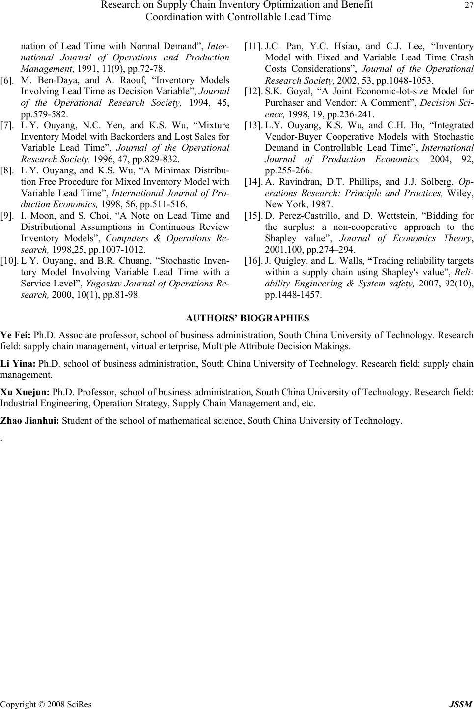

Research on Supply Chain Inventory Optimization and Benefit 27
Coordination with Controllable Lead Time
nation of Lead Time with Normal Demand”, Inter-
national Journal of Operations and Production
Management, 1991, 11(9), pp.72-78.
[6]. M. Ben-Daya, and A. Raouf, “Inventory Models
Involving Lead Time as Decision Variable”, Journal
of the Operational Research Society, 1994, 45,
pp.579-582.
[7]. L.Y. Ouyang, N.C. Yen, and K.S. Wu, “Mixture
Inventory Model with Backorders and Lost Sales for
Variable Lead Time”, Journal of the Operational
Research Society, 1996, 47, pp.8 29-832.
[8]. L.Y. Ouyang, and K.S. Wu, “A Minimax Distribu-
tion Free Procedure for Mixed Inventory Model with
Variable Lead Time”, International Journal of Pro-
duction Economics, 1998, 56, pp.511-516.
[9]. I. Moon, and S. Choi, “A Note on Lead Time and
Distributional Assumptions in Continuous Review
Inventory Models”, Computers & Operations Re-
search, 1998,25, pp.1007-1012.
[10]. L.Y. Ouyang, and B.R. Chuang, “Stochastic Inven-
tory Model Involving Variable Lead Time with a
Service Level”, Yugoslav Journal of Operations Re-
search, 2000, 10(1), pp.81-98.
[11]. J.C. Pan, Y.C. Hsiao, and C.J. Lee, “Inventory
Model with Fixed and Variable Lead Time Crash
Costs Considerations”, Journal of the Operational
Research Society, 2002, 53, pp.1048-1053.
[12]. S.K. Goyal, “A Joint Economic-lot-size Model for
Purchaser and Vendor: A Comment”, Decision Sci-
ence, 1998, 19, pp.236-241.
[13]. L.Y. Ouyang, K.S. Wu, and C.H. Ho, “Integrated
Vendor-Buyer Cooperative Models with Stochastic
Demand in Controllable Lead Time”, International
Journal of Production Economics, 2004, 92,
pp.255-266.
[14]. A. Ravindran, D.T. Phillips, and J.J. Solberg, Op-
erations Research: Principle and Practices, Wiley,
New York, 1987.
[15]. D. Perez-Castrillo, and D. Wettstein, “Bidding for
the surplus: a non-cooperative approach to the
Shapley value”, Journal of Economics Theory,
2001,100, pp.274–294.
[16]. J. Quigley, and L. Walls, “Trading reliability targets
within a supply chain using Shapley's value”, Reli-
ability Engineering & System safety, 2007, 92(10),
pp.1448-1457.
AUTHORS’ BIOGRAP HIES
Ye Fei: Ph.D. Associate professo r, school of busin ess administra tion, South China University of Technolog y. Research
field: supply chain management, virtual enterprise, Multiple Attribute Decision Makings.
Li Yina: Ph.D. school of business administration, South China University of Technology. Research field : supply chain
management.
Xu Xuejun: Ph.D. Professor, school of busin ess administratio n, Sout h China Univ ersity o f Technology. Research f ield:
Industrial Engineering, Operation Strategy, Supply Chain Management and, etc.
Zhao Jianhui: Student of the school of m athematical science, South China University of Technology.
.

2 Fei Ye，Yi-Na Li，Xue-Jun Xu and Jian-Hui Zhao