Paper Menu >>
Journal Menu >>
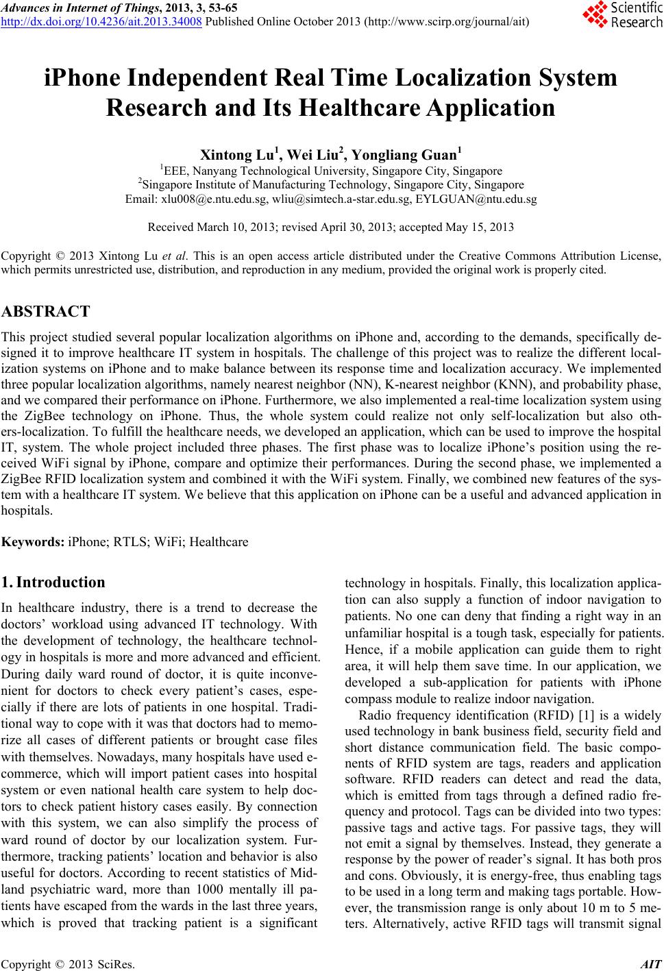 Advances in Internet of Things, 2013, 3, 53-65 http://dx.doi.org/10.4236/ait.2013.34008 Published Online October 2013 (http://www.scirp.org/journal/ait) iPhone Independent Real Time Localization System Research and Its Healthcare Application Xintong Lu1, Wei Liu2, Yongliang Guan1 1EEE, Nanyang Technological University, Singapore City, Singapore 2Singapore Institute of Manufacturing Technology, Singapore City, Singapore Email: xlu008@e.ntu.edu.sg, wliu@simtech.a-star.edu.sg, EYLGUAN@ntu.edu.sg Received March 10, 2013; revised April 30, 2013; accepted May 15, 2013 Copyright © 2013 Xintong Lu et al. This is an open access article distributed under the Creative Commons Attribution License, which permits unrestricted use, distribution, and reproduction in any medium, provided the original work is properly cited. ABSTRACT This project studied several popular localization algorithms on iPhone and, according to the demands, specifically de- signed it to improve healthcare IT system in hospitals. The challenge of this project was to realize the different local- ization systems on iPhone and to make balance between its response time and localization accuracy. We implemented three popular localization algorithms, namely nearest neighbor (NN), K-nearest neighbor (KNN), and probability phase, and we compared their performance on iPhone. Furthermore, we also implemented a real-time localization system using the ZigBee technology on iPhone. Thus, the whole system could realize not only self-localization but also oth- ers-localization. To fulfill the healthcare needs, we developed an application, which can be used to improve the hospital IT, system. The whole project included three phases. The first phase was to localize iPhone’s position using the re- ceived WiFi signal by iPhone, compare and optimize their performances. During the second phase, we implemented a ZigBee RFID localization system and combined it with the WiFi system. Finally, we combined new features of the sys- tem with a healthcare IT system. We believe that this application on iPhone can be a useful and advanced application in hospitals. Keywords: iPhone; RTLS; WiFi; Healthcare 1. Introduction In healthcare industry, there is a trend to decrease the doctors’ workload using advanced IT technology. With the development of technology, the healthcare technol- ogy in hospitals is more and more advanced and efficient. During daily ward round of doctor, it is quite inconve- nient for doctors to check every patient’s cases, espe- cially if there are lots of patients in one hospital. Tradi- tional way to cope with it was that doctors had to memo- rize all cases of different patients or brought case files with themselves. Nowadays, many hospitals have used e- commerce, which will import patient cases into hospital system or even national health care system to help doc- tors to check patient history cases easily. By connection with this system, we can also simplify the process of ward round of doctor by our localization system. Fur- thermore, tracking patients’ location and behavior is also useful for doctors. According to recent statistics of Mid- land psychiatric ward, more than 1000 mentally ill pa- tients have escaped from the wards in the last three years, which is proved that tracking patient is a significant technology in hospitals. Finally, this localization applica- tion can also supply a function of indoor navigation to patients. No one can deny that finding a right way in an unfamiliar hospital is a tough task, especially for patients. Hence, if a mobile application can guide them to right area, it will help them save time. In our application, we developed a sub-application for patients with iPhone compass module to realize indoor navigation. Radio frequency identification (RFID) [1] is a widely used technology in bank business field, security field and short distance communication field. The basic compo- nents of RFID system are tags, readers and application software. RFID readers can detect and read the data, which is emitted from tags through a defined radio fre- quency and protocol. Tags can be divided into two types: passive tags and active tags. For passive tags, they will not emit a signal by themselves. Instead, they generate a response by the power of reader’s signal. It has both pros and cons. Obviously, it is energy-free, thus enabling tags to be used in a long term and making tags portable. How- ever, the transmission range is only about 10 m to 5 me- ters. Alternatively, active RFID tags will transmit signal C opyright © 2013 SciRes. AIT 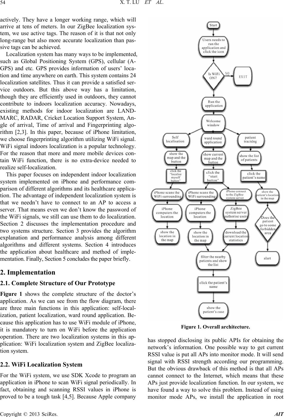 X. T. LU ET AL. 54 actively. They have a longer working range, which will arrive at tens of meters. In our ZigBee localization sys- tem, we use active tags. The reason of it is that not only long-range but also more accurate localization than pas- sive tags can be achieved. Localization system has many ways to be implemented, such as Global Positioning System (GPS), cellular (A- GPS) and etc. GPS provides information of users’ loca- tion and time anywhere on earth. This system contains 24 localization satellites. Thus it can provide a satisfied ser- vice outdoors. But this above way has a limitation, though they are efficiently used in outdoors, they cannot contribute to indoors localization accuracy. Nowadays, existing methods for indoor localization are LAND- MARC, RADAR, Cricket Location Support System, An- gle of arrival, Time of arrival and Fingerprinting algo- rithm [2,3]. In this paper, because of iPhone limitation, we choose fingerprinting algorithm utilizing WiFi signal. WiFi signal indoors localization is a popular technology. For the reason that more and more mobile devices con- tain WiFi function, there is no extra-device needed to realize self-localization. This paper focuses on independent indoor localization system implemented on iPhone and performance com- parison of different algorithms and its healthcare applica- tion. The advantage of independent localization system is that we needn’t have to connect to an AP to access a server. That means even we don’t know the password of the WiFi signals, we still can use them to do localization. Section 2 discusses the implementation procedure and two systems structure. Section 3 provides the algorithm explanation and performance analysis among different algorithms and different systems. Section 4 introduces the application about healthcare and method of imple- mentation. Finally, Section 5 concludes the paper briefly. 2. Implementation 2.1. Complete Structure of Our Prototype Figure 1 shows the complete structure of the doctor’s application. As we can see from the flow diagram, there are three main functions in this application: self-local- ization, patient localization, ward round application. Be- cause this application has to use WiFi module of iPhone, it is mandatory to turn on WiFi before the application operation. There are two localization systems in this ap- plication: WiFi localization system and ZigBee localiza- tion system. 2.2. WiFi Localization System For the WiFi system, we use SDK Xcode to program an application in iPhone to scan WiFi signal periodically. In fact, obtaining and scanning RSSI values in iPhone is proved to be a tough task [4,5]. Because Apple company Figure 1. Overall architecture. has stopped disclosing its public APIs for obtaining the network’s information. One possible way to get current RSSI value is put all APs into monitor mode. It will send signal with RSSI strength according our programming. But the obvious drawback of this method is that all APs cannot connect to the Internet, which means that these APs just provide localization function. In our system, we have found a way to solve this problem. Instead of using monitor mode APs, we install the application in root Copyright © 2013 SciRes. AIT 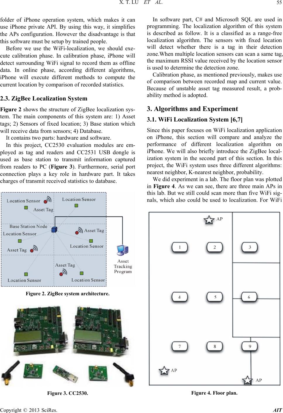 X. T. LU ET AL. 55 folder of iPhone operation system, which makes it can use iPhone private API. By using this way, it simplifies the APs configuration. However the disadvantage is that this software must be setup by trained people. Before we use the WiFi-localization, we should exe- cute calibration phase. In calibration phase, iPhone will detect surrounding WiFi signal to record them as offline data. In online phase, according different algorithms, iPhone will execute different methods to compute the current location by comparison of recorded statistics. 2.3. ZigBee Localization System Figure 2 shows the structure of ZigBee localization sys- tem. The main components of this system are: 1) Asset tags; 2) Sensors of fixed location; 3) Base station which will receive data from sensors; 4) Database. It contains two parts: hardware and software. In this project, CC2530 evaluation modules are em- ployed as tag and readers and CC2531 USB dongle is used as base station to transmit information captured from readers to PC (Figure 3). Furthermore, serial port connection plays a key role in hardware part. It takes charges of transmit received statistics to database. Figure 2. ZigBee system architecture. Figure 3. CC2530. In software part, C# and Microsoft SQL are used in programming. The localization algorithm of this system is described as follow. It is a classified as a range-free localization algorithm. The sensors with fixed location will detect whether there is a tag in their detection zone.When multiple location sensors can scan a same tag, the maximum RSSI value received by the location sensor is used to determine the detection zone. Calibration phase, as mentioned previously, makes use of comparison between recorded map and current value. Because of unstable asset tag measured result, a prob- ability method is adopted. 3. Algorithms and Experiment 3.1. WiFi Localization System [6,7] Since this paper focuses on WiFi localization application on iPhone, this section will compare and analyze the performance of different localization algorithm on iPhone. We will also briefly introduce the ZigBee local- ization system in the second part of this section. In this project, the WiFi system uses three different algorithms: nearest neighbor, K-nearest neighbor, probability. We did experiment in a lab. The floor plan was plotted in Figure 4. As we can see, there are three main APs in this lab. But we still could scan more than five WiFi sig- nals, which also could be used to localization. For WiFi Figure 4. Floor plan. Copyright © 2013 SciRes. AIT 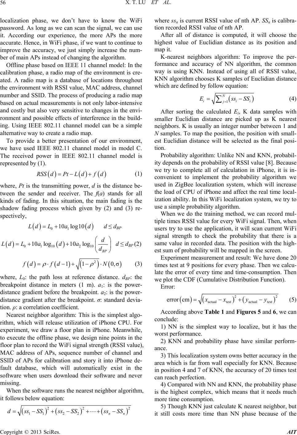 X. T. LU ET AL. 56 localization phase, we don’t have to know the WiFi password. As long as we can scan the signal, we can use it. According our experience, the more APs the more accurate. Hence, in WiFi phase, if we want to continue to improve the accuracy, we just simply increase the num- ber of main APs instead of changing the algorithm. Offline phase based on IEEE 11 channel model: In the calibration phase, a radio map of the environment is cre- ated. A radio map is a database of locations throughout the environment with RSSI value, MAC address, channel number and SSID. The process of producing a radio map based on actual measurements is not only labor-intensive and costly but also very sensitive to changes in the envi- ronment and possible effects of interference in the build- ing. Using IEEE 802.11 channel model can be a simple alternative way to create a radio map. To provide a better presentation of our environment, we have used IEEE 802.11 channel model in model C. The received power in IEEE 802.11 channel model is represented by (1). RSSdPtL dfd (1) where, Pt is the transmitting power, d is the distance be- tween the sender and receiver. The f(a) stands for all kinds of fading. In this situation, the main fading is the shadow fading process which given by (2) and (3) re- spectively, 01 10 log10Ld Lad d ≤ dBP 01 10210 10 log10log BP d Ld Ladad d ≤ dBP (2) 2 11 0,σfd fdN (3) where, L0: the path loss at reference distance. d BP: the breakpoint distance in meters (1 m). a 1: is the power- distance gradient before the breakpoint. a2: is the power- distance gradient after the breakpoint. σ: standard devia- tion. ρ: a correlation coefficient. Nearest neighbor algorithm: This is the simplest algo- rithm, which will release utilization of iPhone CPU. For experiment, we draw a floor plan in iPhone. Meanwhile, to execute the offline phase, we design nine points in the floor plan to record the WiFi signal strength (RSSI value), MAC address of APs, sequence number of channel and SSID of APs for calibration and story it into iPhone de- fault database, which will automatically exist in the software when users download their software and never missing. When the software runs the nearest neighbor algorithm, it follows below equation: 2 22 112 2nn dssSSssSSssSS where ssn is current RSSI value of nth AP. SSn is calibra- tion recorded RSSI value of nth AP. After all of distance is computed, it will choose the highest value of Euclidian distance as its position and map it. K-nearest neighbors algorithm: To improve the per- formance and accuracy of NN algorithm, the common way is using KNN. Instead of using all of RSSI value, KNN algorithm chooses K samples of Euclidian distance which are defined by follow equation: 1 N ii j Ess i SS (4) After sorting the calculated Ei, K data samples with smaller Euclidian distance are picked up as K nearest neighbors. K is usually an integer number between 1 and N samples. To map the position, the position with small- est Euclidian distance will be selected as the final posi- tion. Probability algorithm: Unlike NN and KNN, probabil- ity depends on the probability of RSSI value [8]. Because we try to complete all of calculation in iPhone, it is in- convenient to implement the probability algorithm we used in ZigBee localization system, which will increase the load of CPU of iPhone and affect the real time local- ization ability. In this WiFi localization system, we try to use a simple probability algorithm. When we do the training method, we can record mul- tiple times RSSI value for every WiFi signal. Then, when users try to use the application, it will scan current WiFi signal strength to check the probability that there is a same value in recorded data. The position with the high- est sum of probability will be mapped in the screen. Experiment measurement and result: We have done 20 times test at 9 positions for every phase. Then we calcu- late the error of every time and time-consumption. Then we plot the CDF (Cumulative Distribution Function). Error: 22 actual testactualtest errorcmxx yy (5) According above Table 1 and Figures 5 and 6, we can conclude: 1) NN is the simplest way to localize, but it has the worst performance. 2) KNN and probability phase have similar perform- ance. 3) This localization system owns better accuracy in the area which is far from wall especially for KNN. Because in position 4 and 7 of KNN, the accuracy of 20 times test can reach perfection. 4) Compared with NN and KNN, the probability phase is the highest complex, which means that it needs much more time consumption. 5) Though KNN just calculate K nearest neighbor, but it still costs more time than NN phase because of the Copyright © 2013 SciRes. AIT  X. T. LU ET AL. 57 Table 1. Error distance. NN KNN Probability 1 568.501 244.566 234.078 2 438.353 443.194 263.309 3 510 502.209 553.559 4 403.5 0 39 5 80.077 256.040 267.622 6 168 474.141 341.941 7 622.383 0 187.5 8 418.373 143.012 305.273 9 168 382.5 157.5 Average error distance 375.242 224.566 345.078 Average time consumption 1805 ms 1871 ms 3826 ms Figure 5. Position error distributions. sorting process. 6) According the Figure 6, probability phase has bet- ter performance than others. More than 50% localization points have no error. However, NN phase has the worst error statistics. More than 50% localization points have above 400 cm error distance. 7) For the health care system, since we are focusing on not only the accuracy and but real-time feature, we select KNN as our application phase. Although the test result was good, we still can find that the position of current location may jump to other places Figure 6. Error distance CDF. instantaneously, which has bad performance. Thus, to improve the accuracy, we added a filter to the last result. As the above introduction, the RSSI value may be af- fected by change of circumstance. For instance, if there are many people around the receiver, the RSSI value can change dramatically. According our test, the received RSSI can have 10 dB differences at a same position. Hence, to solve this problem, we store the last several times results as a reference statistics. If the final result is different from the previous data, we should make a deci- sion whether the position should be changed. The logic of the filter is following the diagram Figure 7. Furthermore, to reduce the chance that the display of the position will jump a large-scale distance, we intro- duced a small-scale jump phase. Instead of jumping to the destination point directly, in our system, the position will just move to the inferred point with smaller dis- tance.Because, in our system, the calibration points in the radio map have 397.5 centimeters distance. Although walking speed is various depending on the height, weight, age, terrain, surface, load and so on. The average speed is 5 kilometers per hour, or about 1.3 meters per second. So, imagining a person is walking in our experimental cir- cumstance, the average variation is almost one third of distance of changing. Inferred Position=Original Position Distance Difference +3 (6) where, Distance Difference is the distance between last position and current measured position. Thus, we can track the moving of inferred position. From the above analysis, we know that the probability phase has better performance for the reason that it uses more record statistics. Thus, to improve the NN, KNN performance, we change the calibration phase. Instead of recording the data directly, we adopt a method that it Copyright © 2013 SciRes. AIT  X. T. LU ET AL. 58 Figure 7. Logic of filter. scans the WiFi signal n times and calculate the average RSSI value. In this way, it will avoid the break changing of RSSI value. Meanwhile, to reduce the effect of the direction of devices, we can scan the multi-direction in calibrationphase. When we do the calibration, the user should go round in the position to collect all the statistics of multi-direction. Because we have found that the probability phase has obvious delay. Hence, we just implement above filters and phases in NN and KNN. Then, we did the calibration phase and tested the error distance again just like the previous one. The final ex- perimental resultis as follow: From the final experimental result (Table 2, Figures 8 and 9), we can see that the average error distance of KNN can be reduced to 123.7 cm by mentioned filters and phases. The time consumption will increase a little from 1871 cm to 1925 ms. In addition, because the posi- tion will move small distance every time when the cur- rent position is different from the previous one, the number of small error distance increases. We can see this phenomenon from Figure 9. However, the performance of NN and KNN with filters gets improvement. From Figure 9, the performance of NN with filters is even bet- ter than the performance of probability without filters. It also shows that more than 90 percent of KNN inferred positions with filters have error distance less than 3 meters. The reason why filters can improve the accuracy is that it filters unstable statistics in the radio map. Hence less unexpected jump happens. In addition, the step filter measures the position according human move, which can reduce the large-scale jump. There are still two factors we can explore their rela- tionships with performance, which are the K value of KNN and the number of sampling points. Table 2. Error distance with filter. Error distance Position Index NN KNN 1 329 77 2 214 129 3 251 62 4 480 56 5 270 268 6 77 23 7 416 76 8 91 293 9 49 128 Average error distance 242 124 Average time consumption 1845 ms 1925 ms Figure 8. Position index. Figure 9. Error distance CDF. Copyright © 2013 SciRes. AIT  X. T. LU ET AL. 59 We tested 9 sampling points’ case, and got the statis- tics: From Table 3 and Figure 10, we can know that the K = 4 is the best algorithm for localization in 9 sampling points’ case. Furthermore we can find the average time consumption will increase withthe value of K. Next, for 16 sampling points’ measurement, we got the experimental statistics as follow: From Table 4 and Fig- ure 11, we can easily find that K = 4 is more accurate than others. What’s more, the time consumption still fol- lows the law we got in 9 sampling points. And we also can find that the 16 sampling points will cost more time than 9 sampling locations case. Finally, we tested the 25 sampling points, which is much more complex than others (Table 5).We plotted the average error distance at every location: From Figure 12 and Ta ble 5, we find that the result is different from the earlier two cases. K = 5 has the best result. The reason of this is that the 5th signal is station- ary at the time of the experiment. Furthermore, 25 sam pling points case will be sensitive to any small variation, so K = 4 cannot be as good as 16 sampling points case and 9 sampling points. From all these 9 tests, we can get the following con- clusions: KNN with K = 4 has better result than others generally. 16 sampling points is the best situation. 9 sampling points’ case and 25 sampling points’ case have similar performance in average error distance, Table 3. 9 sampling test statistics. Error distance K = 3 K = 4 K = 5 The Worst Error Distance 379 293 587 Average Error Distance 170 124 186 Average time consumption 1806 ms 1925 ms 1931 ms Figure 10. Average error distance at every location for 9 sampling points. Table 4. 16 sampling points test statistics for 9 sampling points. Error distance K = 3 K = 4 K = 5 The Worst Error Distance 304 256 244 Average Error Distance 134 107 139 Average time consumption 1810 ms 1937 ms 1944 ms Figure 11. Average error distance at every location for 16 sampling points. Table 5. 25 sampling test statistics. Error distance K = 3 K = 4 K = 5 The Worst Error Distance 482 475 340 Average Error Distance 183 179 158 Average time consumption 1891 ms 1971 ms 2663 ms which are worse than 16 sampling points. Although 25 sampling points is more complex, but the statistical si- milarity is too high to get accurate result. K = 3 has the least time-consumption, because after selecting k minimum error distance, it only uses the 3 minimum error distance to localize. For time consumption, 9 sampling points < 16 sam- pling points < 25 sampling points. The reason for this phenomenon is that, for 9 sampling points’ case, it only calculates the distance between current location and 9 recording calibration locations. But for 25 sampling points, it has to compare with 25 recording calibration Copyright © 2013 SciRes. AIT  X. T. LU ET AL. 60 Figure 12. Average error distance at every location for 25 sampling points. locations (Figure 13). We can also find that the bottom points have better accurate than others. The bottom points mean that the measured points near the bottom line of the floor plan. The reason of this result is that around the bottom line there are two APs, which can localize the location accu- rately. At the top of the floor plan there is only one AP. The system hardly finds the accurate location. To im- prove the accuracy of this experimental circumstance, we should add one AP at the top line of the floor plan. 16 sampling points KNN algorithm with K = 4 can achieve 107 cm error distance accuracy. To research the relationship between the K value of KNN and its localization performance, we tested three situations with K = 3, K = 4, K = 5, and plotted their per- formance. According to previous literature, the K value depends on the algorithm, the measurement method and circumstance. We plotted the CDF figures of three cases (Figures 14-16). From the 9 sampling points, we can know that KNN with K = 4 is the best algorithm. From the 16 sampling points, we can know that KNN with K = 4 is the best algorithm. From the 25 sampling points, we can know that KNN with K = 4 has outstanding performance. According to Figure 14-16, we can get the conclusion: Totally, K = 4 has better performance than others. Be- cause, in our experimental circumstance, there are four major routers, they can provide the strong evidence for localization. For RSSI value, the closer distance between Figure 13. Time consumption of each situation. Figure 14. 9 sampling points with different K value. Figure 15. 16 sampling points with different K value. Copyright © 2013 SciRes. AIT  X. T. LU ET AL. 61 Figure 16. 25 sampling points with different K values. APs and receivers, the better stable performance we will get. For K = 5 cases, in 25 sampling points, it has better accuracy than 9 sampling points’ case and 16 sampling points’ case. Because, in 25 sampling points, neighbor distance is smaller than others, it protects against small- scale variation. For the 5th strongest signal, it is not the major signal. Hence, it will experience lots of reflection, diffraction and multipath. It also passes several walls and floors. We can use Ericsson multiple breakpoint model [9] to estimate the remote APs signal. In 9 sampling points, the error distance for different K values is fluctuating. The reason of this phenomenon is that signal surrounding of sampling points in 9 sampling points’ case are quite different. And the distance between points is large. Hence long-distance error can be hap- pened. To research the relationship between the sampling density and its localization accuracy, we also change the sampling density. Instead of 9 sampling points, we use 16 sampling points and 25 sampling points (Figure 17- 19) Then we compare their performance and get the con- clusion. We measured minimum distance between two neigh- bors in there cases: We plotted the above three situations in Figure 20. Then we compared their performance. From Figure 20 and Table 6, we can know that, for short-term distance error, 9 sampling points’ case has better performance than others. For long-term distance error, 16 sampling points’ case is the best one rather than 25 sampling points’ case. We can also find the result of Figure 21 is similar with the previous one. The difference is that in short-term distance error 16 sampling points’ case has similar per- formance with 9 sampling points’ case. Figure 17. 9 sampling points. Figure 18. 16 sampling locations. For K = 5 case, we can also find the conclusion. But the result is clearer than others. In short-term distance error almost half of result in 9 sampling points is zero error. But in long-term case, 16 sampling points is bril- liant. From Figures 20-22, we can get the conclusion: Copyright © 2013 SciRes. AIT  X. T. LU ET AL. 62 Figure 19. 32 sampling locations. Figure 20. Different sampling points with K = 3. Table 6. Minimum neighbors distance. 9 sampling points 16 sampling points 25 sampling points Minimum distance between two neighbors (cm) 330 312 260 9 sampling points has better accuracy or more zero distance in short-term distance error. As we know, 9 sampling points case has far neighbors. It has slim chance to skip to their neighbor, because their neighbors have quite different WiFi circumstance. From minimum neighbors’ distance table, we have gotten the minimum distance between two neighbors. For 9 sampling points’ case, the minimum distance is 330 cm, which is larger than others. However, 16 sampling points’ case and 25 sampling points’ case have outstanding accuracy in long-term. For small probability error, which is long-term distance error, 16 sampling points’ case and 25 sampling points case have common feature that they can protect against the happen of long-term distance error. The reason of this phenomenon is that, for these two cases, they have closer neighbor than 9 sampling points’ case. Even if the meas- ured signal strength is quite different from the calibration strength, it can also find near neighbor to localize. 16 sampling points’ case is more accurate than 25 sampling points. For 25 sampling points, the minimum neighbors distance is too little to localize correctly. The relevant coherency of signal strength between neighbors Figure 21. Different sampling points with K = 4. Figure 22. Different sampling points with K = 5. Copyright © 2013 SciRes. AIT  X. T. LU ET AL. 63 affects its performance. We have already known that, even in same situation, the received strength of same signal source will be different. The range of that is ±10 dB. So for 25 sampling points, it has large probability to skip to its neighbor locations. To find the optimization, we plotted overall CDF fig- ure (Figure 23). We can find the 16 sampling points KNN with K = 4 is the best algorithm. To find the optical number of cali- bration points, we can find the average area for each point. Our experimental lab is 1560 cm × 1620 cm = 2,527,200 cm2. Hence, for each point of 16 sampling points case, we separate the room into 16 areas. Each point covers 2,527,200 ÷ 16 = 157,950 cm2 = 15.795 m2. So we can get the conclusion that, to install localization system like our experimental circumstance, each separated area should cover about 16 m2 and do calibration phase. For value of K, we can get conclusion that the number of K value should be equal to the major APs you have. This system has two subsystems: doctor’s subsystem and patient’s subsystem. For patient’s subsystem, because this system is used as self-localization and self-navigation, as users, they can clearly tell the small distance error and subjectively tell which is the correct location. We just care about long- term distance error. From Figure 23, we can know 16 sampling points KNN algorithm with K = 4 is the best one. We will adopt this method in our healthcare applica- tion in chapter V. For doctor’s subsystem, because it is used as ward round case filter, it should be very accurate in small-term distance and of high-resolution ratio to tell the difference form patient to patient. Thus we selected 25 sampling points with K = 4 as the algorithm. Since there are lots of other future functions of this application, we can select different algorithm according to the requirement of the application. 3.2. ZigBee Localization System [10] In the ZigBee localization system, we used Improved Bayesian probability radio map algorithm. Because we did this in the server, we needn’t care more about the complexity of the algorithm. Thus, improving the accu- racy is the target. We assume that the value received by every location sensor belongs Gaussian Distribution. The equation for mean and deviation is shown below: 1 μ n i i x n (7) 2 1μ σ n i ix n (8) 2 2 1e2σ σ2π x fx (9) where xi is an RSSI value; μ is the mean value of sample RSSI value σ is the standard deviation of sample RSSI value. According the Gaussian Distribution, when the base station receives a RSSI packet, it can compute the prob- ability of current value in each location sensor. Finally the position with highest probability will be assigned to the final position. Improved Bayesian Probability Radio Map Algorithm [10]: The probabilistic approach for radio map algorithm can be realized by using the concept of, conditional probability, Bayes theorem (Figure 24). The formula used for computing the likelihood for each position of the asset tag is shown below: ii in jj j PBAPA PAB PBAPA (10) where: N is the number of location points of the radio map; P(Ai) is the probability that the object is at the par- ticular point I; P(BAj) is the probability that the particu- lar RSSI value B is received at a particular point I; P(AiB) is the probability that the object is in a particular point I given the received RSSI value B. Figure 23. Overall performance. Figure 24. Block diagram of improved bayesian probability radio map algorithm. Copyright © 2013 SciRes. AIT  X. T. LU ET AL. 64 When the reader received the RSSI value, it would first convert the values into a probability value for each calibration point using “probabilistic map”. A “condi- tional probability map” could then be calculated by using the probability values from the previous step. A condi- tional probability map contained probability that the asset tag would be for each calibrated point shown below. The position of the highest probability would be deemed as the position of the object. Position Inference Algorithm: The algorithm would take into consideration a number of calibration points that locate near the test point, instead of just the nearest calibration point, during computation shown below. It was based on the assumption that points, which were located close together, had relatively similar RSSI signa- ture values. The final “inferred” position was then computed in a function that involved the probability of each points and distances between the considered points. To improve the accuracy, we combined the two algo- rithms. The result of the nine test points has shown in below table. According to Table 7, the average error distance is 28.25cm, which is much better than the WiFi system. 4. Healthcare Application To combine this system with healthcare application, we must find the demands. It is common for doctors to carry patient’s case during daily ward round. So our target is to simply the work of doctors. When users click the health- care button and switch the localization button on, it will map current self-location and all patients’ location. Fig- ure 25 Then doctors can click nearby button to view sur- rounding patients’ list. For instance, when the doctor stand by the patient A if he is trying to check in the di- agnosis of patient A. he can press the “nearby” button and then he can easily find patient A from the nearby list, nevertheless, patient B who is far from the doctor or even in another ward will not be listed in the nearby list. (Fig- ure 26) This will definitely improve the efficiency of doctors’ work. Furthermore, this application can also remind doctors which patients have been checked and which one has not. If the doctor has checked the patient, the doctor can mark it. It will not display on the screen until the end of this ward round. Further more, this application can also develop a sub-application for patients for indoor navigation. To help patients to find right direction and right way, we also use the compass in iPhone, which will help both doctors and patients to find the direction. Especially, for patient, who newly come to a hospital. It is quite difficult for them to find a right place and room to deal with the hospital issues. For instance, for patients, who should take X-ray in diagnostic imaging department. But Table 7. Test results of ZigBee location system. NOActual PositionMeasured PositionError Distance (cm) 1(100,350)(100,350)0 2(100,700)(150,760)78.102 3(2,001,150)(2,001,150)0 4(400,140)(400,140)0 5(400,950)(470,980)76.158 6(550,250)(550,250)0 7(55,050)(550,550)0 8(550,800)(550,700)100 9(5,501,050)(5,501,050)0 Figure 25. Doctor’s application. there are lots of departments in a hospital and there may be crowded which proves inconvenient for patients. With this application, nevertheless, patients don’t have to worry about loss their way in hospitals. It can guide pa- tients to go to right place. As we can see from the picture, the array direction is the direction that the patient is fac- ing. The other function of this application is to track pa- tients (Figure 27). For mental disease patients, they need to be tracked to prevent accidents and escape from hos- pital. Hence setting some restricted zone is necessary to alert doctors to their patients’ unusual locations and be- haviors. In the tracking function, if a patient goes into restricted area, the application will alert. Copyright © 2013 SciRes. AIT  X. T. LU ET AL. Copyright © 2013 SciRes. AIT 65 Figure 26. Nearby patient’s list. Figure 27. Navigation function. 5. Conclusion To be more practical and efficient, the next step is to use it in hospital to verify its result. Furthermore, to improve the accuracy, adding more APs is an effective way. However, it will increase the time delay during localiza- tion, which will decrease the real-time sensitivity. So we should find a balance between the accuracy, sensitivity and complexity of a practical real-time RTLS system. REFERENCES [1] L. M. Ni, Y. H. Liu, Y. C. Lau and A. P. Patil, “LAND- MARC: Indoor Location Sensing Using Active RFID,” Proceedings of the 1st IEEE International Conference on Pervasive Computing and Communications, March 2003. [2] J. Wyffels, J.-P. Goemaere, P. Verhoeve, P. Crombez, B. Nauwelaers, L. DeStrycker, K. A. H. O. Sint-Lieven, K. U. Leuven and N. V. Televic, “A Novel Indoor Localiza- tion System for Healthcare Environments,” International Symposium on Computer-Based Medical Systems (CBMS), 2012. [3] M. Pourhomayoun, Z. P. Jin and M. Fowler, “Spatial Sparsity Based Indoor Localization in Wireless Sensor Network for Assistive Healthcare,” IEEE International Conference on Engineering in Medicine and Biology So- ciety (EMBC), 2012. [4] M. Bharanidharan, X. J. Li, Y. Y. Jin, J. S. Pathmasun- tharam and G. X. Xiao, “Design and Implementation of a Real Time Locating System Utilizing WiFi Signals from iPhones,” IEEE International Conference on Networks (ICON), 2012. [5] M. Ali, “iPhone SDK Programming: Developing Mobile Applications for Apple iPhone and iPod Touch,” Wiley Press, 2009. [6] Q. X. Chen; D.-L. Lee and W.-C. Lee, “Rule-Based WiFi Localization Methods,” IEEE/IFIP International Confer- ence on Embedded and Ubiquitous Computing, 2008. [7] T. Bagosi and Z. Baruch, “Indoor Localization by WiFi,” IEEE International Conference on Intelligent Computer Communication and Processing (ICCP), 2011. [8] Effelsberg, “COMPASS: A Probabilistic Indoor Posi- tioning System Based on 802.11 and Digital Compasses,” WiNTECH ‘06 Proceedings of the 1st International Workshop on Wireless Network Testbeds, Experimental Evaluation & Characterization, 2006, pp. 34-40. [9] W.-H. Chen, H. H. Chang; T. H. Lin, P. C. Chen, L. K. Chen, S. J. Hwang, D. H. J. Yen, H. S. Yuan and W. C. Chu, “Dynamic Indoor Localization Based on Active RFID for Healthcare Applications: A Shape Constraint Approach,” International Conference on Biomedical En- gineering and Informatics (BMEI), 2009. [10] L. Y. Hao, G. Y. Liang and L. Wei, “Indoor Positioning system ( Middleware),” Nanyang Technological Univer- sity, Nanyang, 2012. |