An Extension to Pi-Calculus for Performance Evaluation

doi:10.4236/jsea.2011.41002

Paper Menu >>

Journal Menu >>

Journal of Software Engineering and Applications, 2011, 1, 9-17

doi:10.4236/jsea.2011.41002 Published Online January 2011 (http://www.scirp.org/journal/jsea)

An Extension to Pi-Calculus for Performance

Evaluation

Shahram Rahimi, Elham S. Khorasani, Yung-Chuan Lee, Bidyut Gupta

Department of Computer Science, Southern Illinois University, Illinois, USA.

Email: {rahimi, elhams, yclee, bidyut}@siu.edu

Received October 12th, 2010; revised November 25th, 2010; accepted November 30th, 2010.

ABSTRACT

Pi-Calculus is a formal method for describing and analyzing the behavior of large distributed and concurrent systems.

Pi-calculus offers a conceptual framework for describing and analyzing the concurrent systems whose configuration

may change during the computation. With all the advantages that pi-calculus offers, it does not provide any methods for

performance evaluation of the systems described by it; nevertheless performance is a crucial factor that needs to be

considered in designing of a multi-process system. Currently, the available tools for pi-calculus are high level language

tools that provide facilities for describing and analyzing systems but there is no practical tool on hand for pi-calculus

based performance evaluation. In this paper, the performance evaluation is incorporated with pi-calculus by adding

performance primitives and associating performance parameters with each action that takes place internally in a sys-

tem. By using such parameters, the designers can benchmark multi-process systems and compare the performance of

different architectures against one another.

Keywords: Pi-calculus, Performance Evaluation, Multi-Agent Systems, System Modeling

1. Introduction

Pi-calculus, introduced by Robin Milner [1-5], stands out

as one of the most powerful modeling tools for modeling

and analyzing the behavior of concurrent computational

systems such as: multi agent systems, grid computing sy-

stems, and so forth. Pi-calculus defines the syntax of pro-

cesses and actions and provides transition rules for ana-

lyzing and validating system functionalities. Mobility in

pi-calculus is achieved by sending and receiving channel

names through wh ich the recipient can co mmunicate with

the sender or even with other processes, provided the

channel is a free name. With the interaction between the

processes changing, the configuration of the whole sys-

tem is also changed and mobility is attained . In the high-

er-order pi-calculus [5], computational entities (such as

objects, process, or a code segment) can be transferred as

well as the values and channel names. Because of its

strong support for mobility, higher order pi-calculus is

very flexible and powerful in modeling mobile agen t sys-

tems. As mentioned before, however, pi-calculus by it-

self does not provide any method for performance evalu-

ation of systems described by it; nevertheless, perfor-

mance is an important factor that needs to be considered

in designing of a multi-process system. The traditional

software development methods delay the performance

test until after the implementation is completed. This

approach has its obvious drawback as if the system is

found not satisfying the desired performance require-

ments, then most of the implementation has to be redone.

So evaluating the performance at the design stage has

significant importance and can save much of the devel-

opers’ time, energy and cost.

The previous works for integrating th e process algebra

with performance measures have either extended the syn-

tax and semantics of the pi-calculus to account for per-

formance, or derived quantitative performance measures

from the system transitions.

In the former approach, a family of stochastic process

algebra [6-14] has been introduced that extends the stan-

dard process algebra with timing or probability informa-

tion. In this algebra, ev ery action has an associated dura-

tion which is assumed to be a random variable with an

exponential distribution. A prefix then is in the form of

(a,r).P, where a represents an action with a duration that

is exponentially distributed with parameter r, known as

the action rate. The memory-less property of the expo-

nential distribution conforms to the Markov property thus

Markov chains [15-16] are applied to compute the prob-

ability of reaching each state. Consequently, the final

An Extension to Pi-Calculus for Perf orm anc e E valuation

performance of the system can be calculated given the

reward model. One potential problem with providing

explicit action rates is that when the action rates are not

known in advance, a different symbol is used for each

action rate which leads to a heavy computational over-

head in performance calculation.

In the latter approach [17-18], labels of the transition

systems are enhanced to carry additional information

about the inference rule which was applied to the transi-

tion. So instead of giving an explicit action rate for each

action, the probabilistic distributions are computed from

the transition labels by associating a cost function to each

transition. Then Marko v chain is app lied as before to cal-

culate the final performance.

In this paper we follow the latter approach, in that we

leave the syntax of the pi-calculus intact and associate

performance parameters with each inference rule. How-

ever, our approach differs from the previous works in

two aspects: first, the cost functions proposed in the pre-

vious works are too abstract to be directly applied to real

cases. Thus, in this paper a cost function is replaced by a

concrete transition rate function that estimates the dura-

tion time for each transition rule. Second, our transition

rates account for process mobility such as transferring

objects or codes from one environment to another, con-

sidering the fact that the process mobility (suc h as mobile

agents) is different from simple name exchange in its

complexity and additional overhead [19].

The rest of the paper is organized as follows: we start

with some background knowledge on pi-calculus syntax

and its transition rules. Then we review the continuous

time Markov chains, their steady state analysis and re-

ward models. Finally, we introduce the transition rate

function and establish our performance evaluation me-

thodology based on it. A conclusion section summaries

the paper at the end and gives a prospective for future

work in this area.

2. Pi-Calculus

Pi-calculus, an extension of the process algebra CCS, was

introduced by Robin Milner in the late 80 s [1]. It provides

a formal theory for modeling mobile systems and reason-

ing about their behaviors. In pi-calculus, two entities are

specified, “names” and “processes” (or “agents”). “Na me”

is defined as a channel or a value that is transferred via a

channel. We follow the naming conventions and the syn-

tax of [1] in wh ich u, v, w, x, y, z range over names and A,

B, C,  range o ver process (agent) identi fiers.

The syntax of an agent (or a process) in pi-calculus is

defined as follows:







12 1

::0. ().. .

,, !

PPyxPyxPyxPPPP

PPxPxyPAyy P













 0 is a null process and means that agent P does not

do anything.

 .

iI P







: Agent P will behave as either one of



whereiI



, but not more than one, and the-

behaves likei

P. If



, then P behaves like 0.

 Here i



denotes any actions that could take place

in P (such as



,()yx, and so on).

 Here i



denotes any actions that could take place

in P (such as



,()yx, and so on).

 .

xP: Agent P sends the free name x out along

channel y and then behaves like P.

 Nam e x is said to be free if it is not bound to agent P.

In the same way, if x is bound to P (also say private

to P), that means x can only be used inside by P.







: Agent P sends bound name x out along

channel y and then behaves like P.







: Agent P receives name x along channel y

and then behaves like P.

 .P



: Agent P performs the silent action



and

then behaves like P.

 12

PP: Agent P has 1

P and 2

P executing in paral-

lel. 1

P and 2

P may behave independently or they

may interact with each other. E.g. if 111

.PP





and

222

.PP





, then 1

P and 2

P will behave indepen-

dently. But, if 11

().PyxP



and



.PyxP then

P sends name x to 2

Pvia channel y.

 The sum 12



means either 1

P or 2

P is ex-

ecuted, but not both.







P: is called restriction and means that agent P

does not change except for that x in P becomes pri-

vate to P. That means any outside communication

through channel x is proh ibited.

 A match operator [x = y] P means tha t if x = y, then

the agent behaves like P, otherwise it behaves like 0.







1,,

yy is an agent identifier where

1,,

yy are free names occurring in P.

 !P is called replication and can be thought of as an

infinite compositio nPPP.

The semantics of the calculus is defined by a set of

transition rules which establish the system evolution. A

transition rule is in the form of '



, which

means that process P evolves to '

Pafter performing ac-

tion



. Action



can be one of the following prefix-

es:





:: yx yxyx







Pi-calculus transition rules are listed in Table 1. The

TAU-ACT, INPUT-ACT, OUTPUT-ACT, SUM and

MATCH rules correspond directly to the definition of the

silent, input, and output actions and the sum and match

operators. The side condition



wfnzP in the

INPUT-ACT rule ensures that a free occurrence of w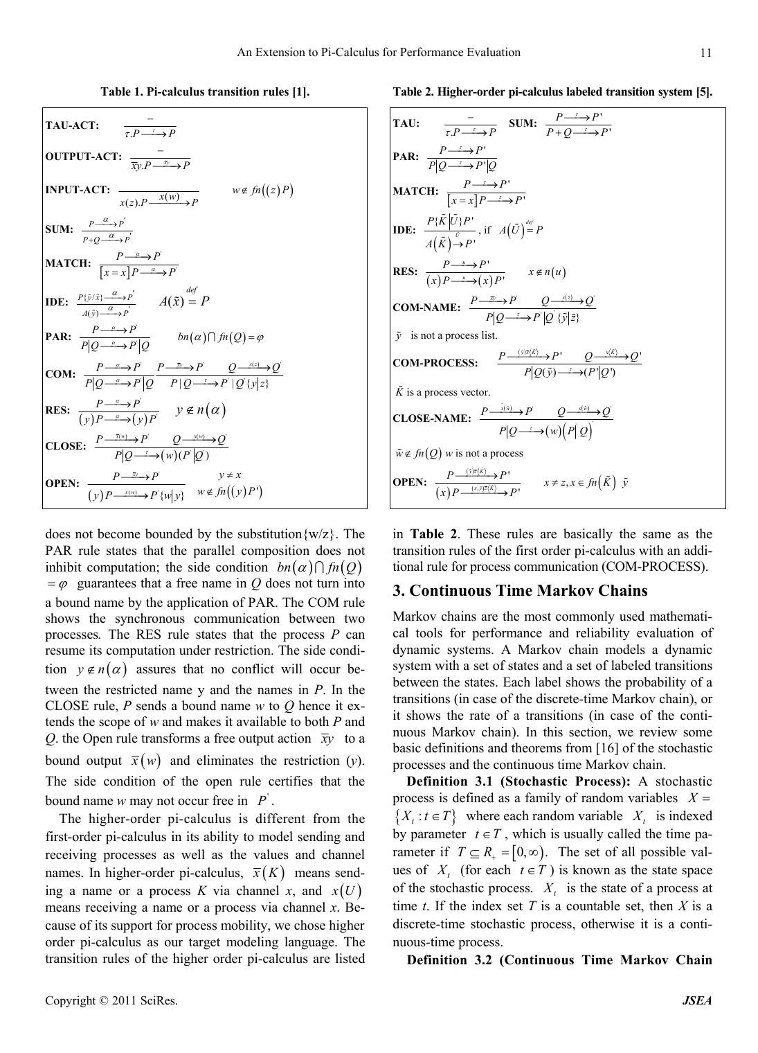

An Extension to Pi-Calculus for Perf orm anc e E valuation

Table 1. Pi-calculus transition rules [1].

TAU-ACT: .PP







OUTPUT-ACT: .xy

yP P





INPUT-ACT: ()

(). xw

zP P



wfnzP

SUM: '







MATCH:



xP P







IDE: '

{/}

()

yx P

Ay P







 ()

def

xP



PAR: '

PQP Q





 

bnfn Q







COM:



'' '

'||{}

PPPPQ Q

PQPQ yz

PQP Q









RES:

 

yP yP











CLOSE:

 



()

xw xw

PPQQ

PQwP Q







OPEN:



() {}

yP Pwy







wfnyP





does not become bounded by the substitution{w/z}. The

PAR rule states that the parallel composition does not

inhibit computation; the side condition







bnfn Q







 guarantees that a free name in Q does not turn into

a bound name by the ap plication of PAR. The COM rule

shows the synchronous communication between two

processes. The RES rule states that the process P can

resume its computation under restriction. The side condi-

tion





 assures that no conflict will occur be-

tween the restricted name y and the names in P. In the

CLOSE rule, P sends a bound name w to Q hence it ex-

tends the scope of w and makes it available to both P and

Q. the Open rule transforms a free output action

y to a

bound output



w and eliminates the restriction (y).

The side condition of the open rule certifies that the

bound name w may not occur free in '

The higher-order pi-calculus is different from the

first-order pi-calculus in its ability to model sending and

receiving processes as well as the values and channel

names. In higher-order pi-calculus,



K means send-

ing a name or a process K via channel x, and





means receiving a name or a process via channel x. Be-

cause of its support for process mobility, we chose higher

order pi-calculus as our target modeling language. The

transition rules of the higher order pi-calculus are listed

Table 2. Higher -order pi -calcu lus labeled tr ansitio n syst em [5].

TAU: .PP





 SUM: '

PQ P







PAR: '

PQP Q





MATCH:



xP P







IDE:



{}'

PKUP

KP





, if



def





RES:

 

xP xP





COM-NAME:



'{}

PPQ Q

PQP Qyz











 is not a process list.

COM-PROCESS:



()( '')

yxK xK

PPQQ

PQ yPQ



 







is a process vector.

CLOSE-NAME:

 



xw xw

PPQQ

PQwP Q















wfnQ

w is not a process

OPEN:



yzK

xyzK

zx fnK y

xP P









in Table 2. These rules are basically the same as the

transition rules of the first order pi-calculus with an addi-

tional rule for process communication (COM-PROCESS).

3. Continuous Time Markov Chains

Markov chains are the most commonly used mathemati-

cal tools for performance and reliability evaluation of

dynamic systems. A Markov chain models a dynamic

system with a set of states and a set of labeled transitions

between the states. Each label shows the probability of a

transitions (in case of the discrete-time Markov chain), or

it shows the rate of a transitions (in case of the conti-

nuous Markov chain). In this section, we review some

basic definitions and theorems from [16] of the stochastic

processes and the continuous time Markov chain.

Definition 3.1 (Stochastic Process): A stochastic

process is defined as a family of random variables







tT where each random variable t

is indexed

by parameter tT



, which is usually called the time pa-

rameter if





0, .TR



 The set of all possible val-

ues of t

(for each tT



) is known as the state space

of the stochastic process. t

is the state of a process at

time t. If the index set T is a countable set, then X is a

discrete-time stochastic process, otherwise it is a conti-

nuous-time process.

Definition 3.2 (Continuous Time Markov Chain

An Extension to Pi-Calculus for Perf orm anc e E valuation

(CTMC)): A stochastic process



tTconstitutes a

CTMC if it satisfies the Markov property, namely that,

given the present state, the future and the past states are

independent. Formally, for an arbitrary 0



 with

01 1

tttt nN



  and 0

sS , the

following relation holds for the conditional probability

mass function (pmf):



1 10

,,,

nnn

tntntnt

tntn

PXsXs XsXs

PXsXs



 





where



tntn

PXsXs



 is the transition proba-

bility to travel from state n

Sto state 1n

S during the

period of time





.

Definition 3.3 (Time-homogenous CTMC): A

CTMC is called time-homogenous if the transition prob-

abilities



tntn

PXsXs



 depend only on the

time difference tn+1-tn, and not on the actual values of tn+1

and tn.

Definition 3.4 (State Sojourn Time): The sojourn

time of a state is the time spent in that state before mov-

ing to another state. The sojourn time of time-homo-

genous CTMC exhibits the memory less property. Since

the exponential distribution is the only continuous distri-

bution with this property, the random variables denoting

the sojourn times, or holding times, must be exponen-

tially distributed.

Definition 3.5 (Irreducible CTMC): A CTMC is

called irreducible if every state i

S is reachable from

every other state i

S, that is:



,,, 0:0

ijijij

SSSStp t

Definition 3.6 (Instantaneous Transition Rates of

CTMC): A transition rate





q, measures how quickly

a process travels from state i to state j at time t. The tran-

sition rates are related to the conditional transition prob-

abilities as follows:





lim ,

() (,) 1

lim ,

ij ij ij

tij

ptt tij

qt ptt tqij



 

















(3.1)

The instantaneous transition rates form the infinitesimal

generator matrix ij





A CTMC can be mapped in to a directed graph, where

the nodes represent states and the arcs represent transi-

tions between the states labeled by their transition rates.

Definition 3.7 (The State Probability Vector): The

state probability vector is a probability vector



ttt



, where i



is the probability that the

process is in state i

S at time t. Given the initial state

probability,







, the state probability vector at

time t is calculated as:





00, 0

tPt t





 (3.2)

Because of the continuity of time, Equation (3.2) cannot

be easily solved; instead the following differential equa-

tion is used [16] to calculate the state probability vector

from the transition rates:





ij i

tttt





 (3.3)

3.1. The Steady State Analysis

For evaluating the performance of a dynamic system, it is

usually desired to analyze th e behavior of the system in a

long period of execution. The long run dynamics of

Markov chains can be studied by finding a steady state

probability vecto r.

Definition 3.8 (The Steady State Probability Vecto r):

The state probability vector



is steady if it does not

change over time. This means that further transitions do

not affect the steady state probabilities, and :





lim 0







, where





is the steady state prob-

ability vector. Hence from Equatio n (3.3):

 

ij i

qt tjS









, or in vector matrix form:



 (3.4)

Thus the steady state probability vector, if existing, can

be uniquely determined by the solution of Equation (3.4),

and the condition1







.

The following theorem states the sufficient conditions

for the existence of a unique steady-state probability

vector.

Theorem 3.1: a time-homegenous CTMC has a unique

steady-state probability vector if it is irreducible and finite.

A CTMC for which a unique steady state probability

vector exists is called an ergodic CTMC. In an ergodic

CTMC, each state is reachable from any other states

through one or more steps. The steady-state probability

vector



for an ergodic CTMC can be found directly

by solving Equation (3.4) as illustrated by the following

example:

Figure 1 shows an ergodic CTMC containing five

states: 12345

,,,,SSSSS when each state is reachable

from other states. The value associated with each arc is

the instantaneous transition rate between the states. The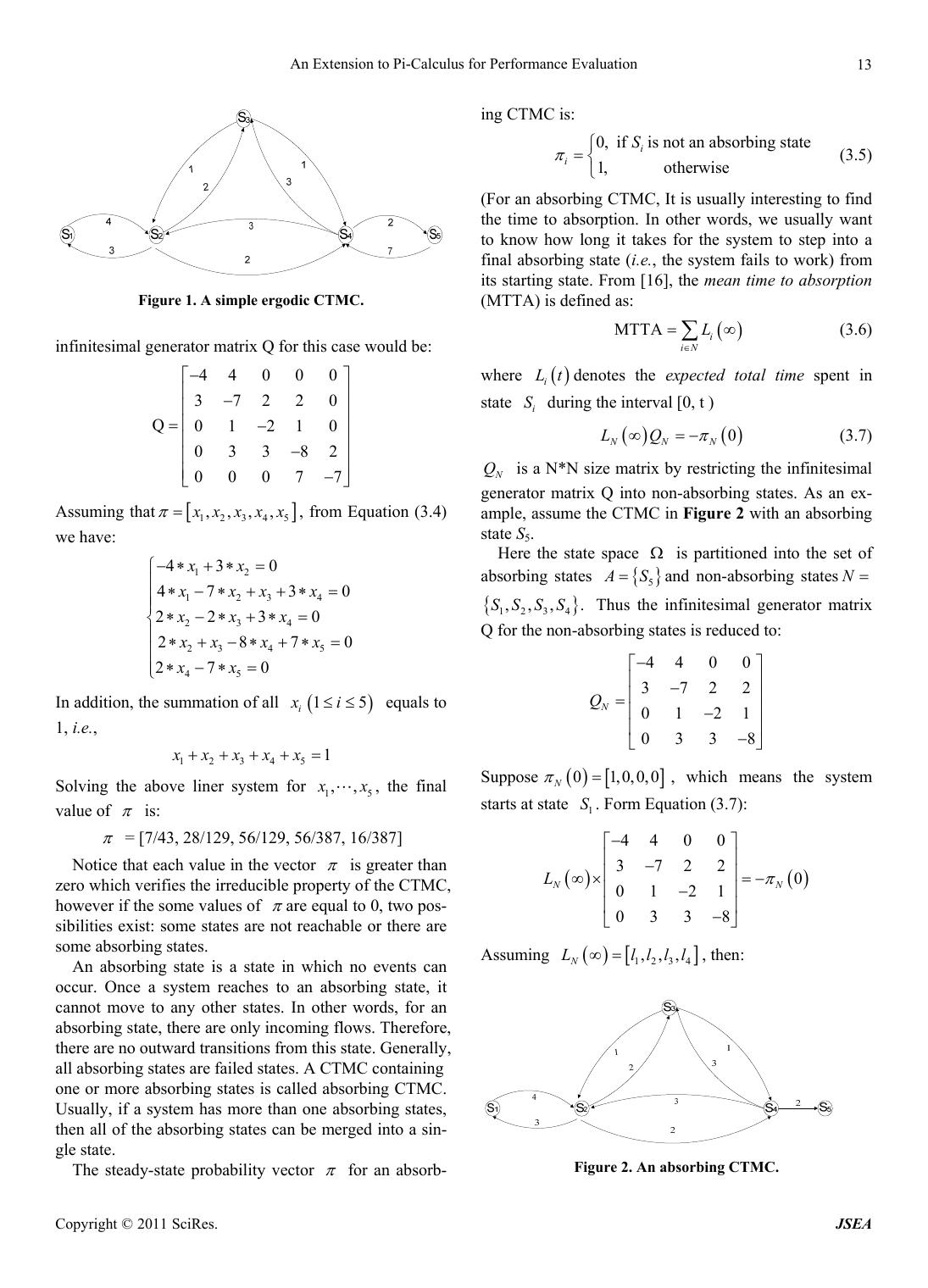

An Extension to Pi-Calculus for Perf orm anc e E valuation

Figure 1. A simple ergodic CTMC.

infinitesimal generator matrix Q for this case would be:

44 0 0 0

37220

Q01 210

033 82

0007 7























Assuming that





12345

,,,,

xxxx



, from Equation (3.4)

we have:

1234

234

23 45

43 0

473 0

2230

2870

270

xxx x

xxx

xx xx

 



 















In addition, the summation of all



xi equals to

1, i.e.,

12345

1xxxxx 

Solving the above liner system for 15

x, the final

value of



is:



= [7/43, 28/129, 56/129, 56/387, 16/387]

Notice that each value in the vector



is greater than

zero which verifies the irreducible property of the CTMC,

however if the some values of



are equal to 0, two pos-

sibilities exist: some states are not reachable or there are

some absorbing states.

An absorbing state is a state in which no events can

occur. Once a system reaches to an absorbing state, it

cannot move to any other states. In other words, for an

absorbing state, there are only incoming flows. Therefore,

there are no outward transitions from this state. Generally,

all absorbing states are failed states. A CTMC containing

one or more absorbing states is called absorbing CTMC.

Usually, if a system has more than one absorbing states,

then all of the absorbing states can be merged into a sin-

gle state.

The steady-state probability vector



for an absorb-

ing CTMC is:

0,ifis not an absorbing state

1, otherwise







 (3.5)

(For an absorbing CTMC, It is usually in teresting to find

the time to absorption. In other words, we usually want

to know how long it takes for the system to step into a

final absorbing state (i.e., the system fails to work) from

its starting state. From [16], the mean time to absorption

(MTTA) is defined as:



MTTA i







 (3.6)

where





Ltdenotes the expected total time spent in

state i

S during the interval [0, t )





NNN



 (3.7)

Q is a N*N size matrix by restricting the infinitesimal

generator matrix Q into non-absorbing states. As an ex-

ample, assume the CTMC in Figure 2 with an absorbing

state S5.

Here the state space



is partitioned into the set of

absorbing states





Sand non-absorbing statesN







1234

,,, .SSSS Thus the infinitesimal generator matrix

Q for the non- ab sorbing states is reduc ed to:

44 00

3722

01 21

033 8



































Suppose









0 1,0,0,0



, which means the system

starts at state 1

S. Form Equation (3.7):

 

44 0 0

3722 0

01 21

033 8













 











Assuming









1234

,,,

Lllll , then:

Figure 2. An absorbing CTMC.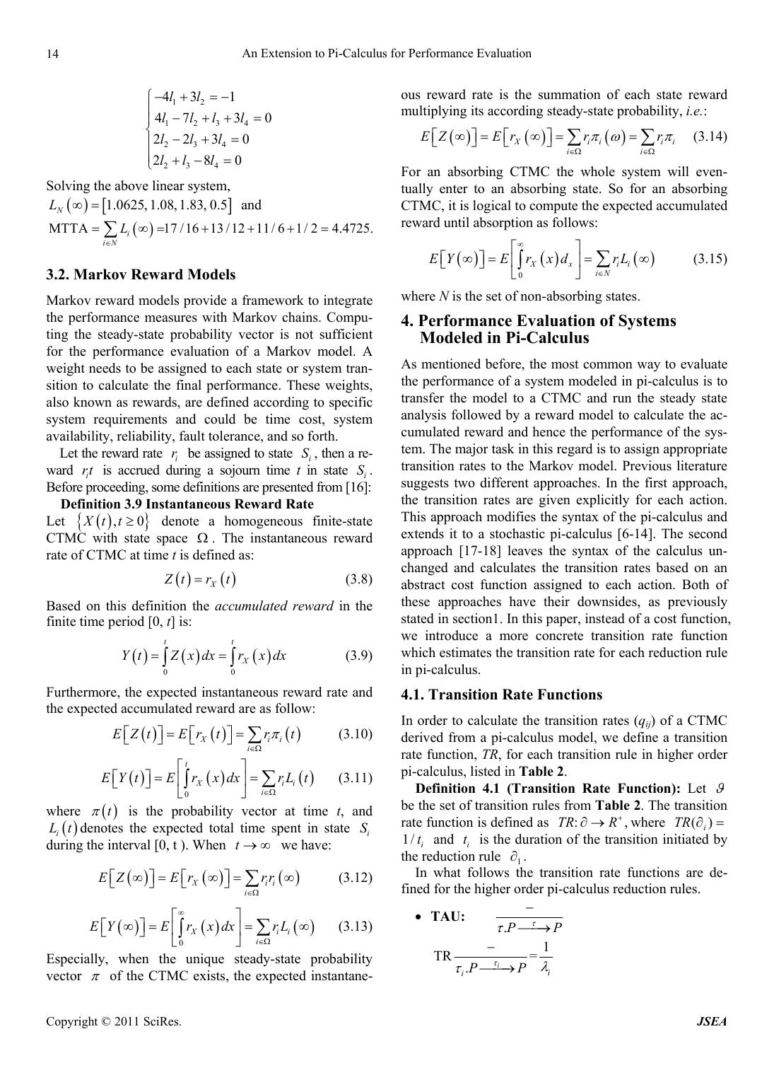

An Extension to Pi-Calculus for Perf orm anc e E valuation

1234

234

23 4

431

4730

2230

280

llll

lll

ll l

 















Solving the above linear system,







1.0625,1.08,1.83,0.5

L and



MTTA17/16 13/12 11/6 1/24.4725.







3.2. Markov Reward Models

Markov reward models provide a framework to integrate

the performance measures with Markov chains. Compu-

ting the steady-state probability vector is not sufficient

for the performance evaluation of a Markov model. A

weight needs to be assigned to each state or system tran-

sition to calculate the final performance. These weights,

also known as rewards, are defined according to specific

system requirements and could be time cost, system

availability, reliability, fault tolerance, and so forth.

Let the reward rate i

r be assigned to state i

S, then a re-

ward i

rt is accrued during a sojourn time t in state i

Before p roceedi ng, som e defi nitio ns are pr esente d from [16]:

Definition 3 . 9 Instantaneou s Reward Rate

Let





,0Xt t denote a homogeneous finite-state

CTMC with state space . The instantaneous reward

rate of CTMC at time t is defined as:







trt (3.8)

Based on this definition the accumulated reward in the

finite time period [0, t] is:

 

YtZx dxrx dx



(3.9)

Furthermore, the expected instantaneous reward rate and

the expected accumulated reward are as follow:

 

Xii

EZtErtrt







 

 

 (3.10)

 

Xii

EYtErxdxrL t











 (3.11)

where





is the probability vector at time t, and



Ltdenotes the expected total time spent in state i

during the interval [0, t ). When t we have:

 

Xii

EZ Errr



 

 

 

 (3.12)

 

0Xii

EYEr xdxrL







 







 (3.13)

Especially, when the unique steady-state probability

vector



of the CTMC exists, the expected instantane-

ous reward rate is the summation of each state reward

multiplying its according steady-state probability, i.e.:









Xiiii

EZ Errr





 

 

 

 



(3.14)

For an absorbing CTMC the whole system will even-

tually enter to an absorbing state. So for an absorbing

CTMC, it is logical to compute the expected accumulated

reward until absorption as follows:

 

0Xx ii

EYEr xdrL

















 (3.15)

where N is the set of non-absorbing states.

4. Performance Evaluation of Systems

Modeled in Pi-Calculus

As mentioned before, the most common way to evaluate

the performance of a system modeled in pi-calculus is to

transfer the model to a CTMC and run the steady state

analysis followed by a reward model to calculate the ac-

cumulated reward and hence the performance of the sys-

tem. The major task in this regard is to assign appropriate

transition rates to the Markov model. Previous literature

suggests two different approaches. In the first approach,

the transition rates are given explicitly for each action.

This approach modifies the syntax of the pi-calculus and

extends it to a stochastic pi-calculus [6-14]. The second

approach [17-18] leaves the syntax of the calculus un-

changed and calculates the transition rates based on an

abstract cost function assigned to each action. Both of

these approaches have their downsides, as previously

stated in section1. In this paper, instead of a cost function,

we introduce a more concrete transition rate function

which estimates the transition rate fo r each reduction rule

in pi-calculus.

4.1. Transition Rate Functions

In order to calculate the transition rates (qij) of a CTMC

derived from a pi-calculus model, we define a transition

rate function, TR, for each transition rule in higher order

pi-calculus, listed in Table 2.

Definition 4.1 (Transition Rate Function): Let



be the set of transition rules from Table 2. The transition

rate function is defined as :,TR R

 where ()





1/ i

t and i

t is the duration of the transition initiated by

the reduction rule 1



In what follows the transition rate functions are de-

fined for the higher order pi-calculus reduction rules.

 TAU: .PP







TR 1

.ii

iPP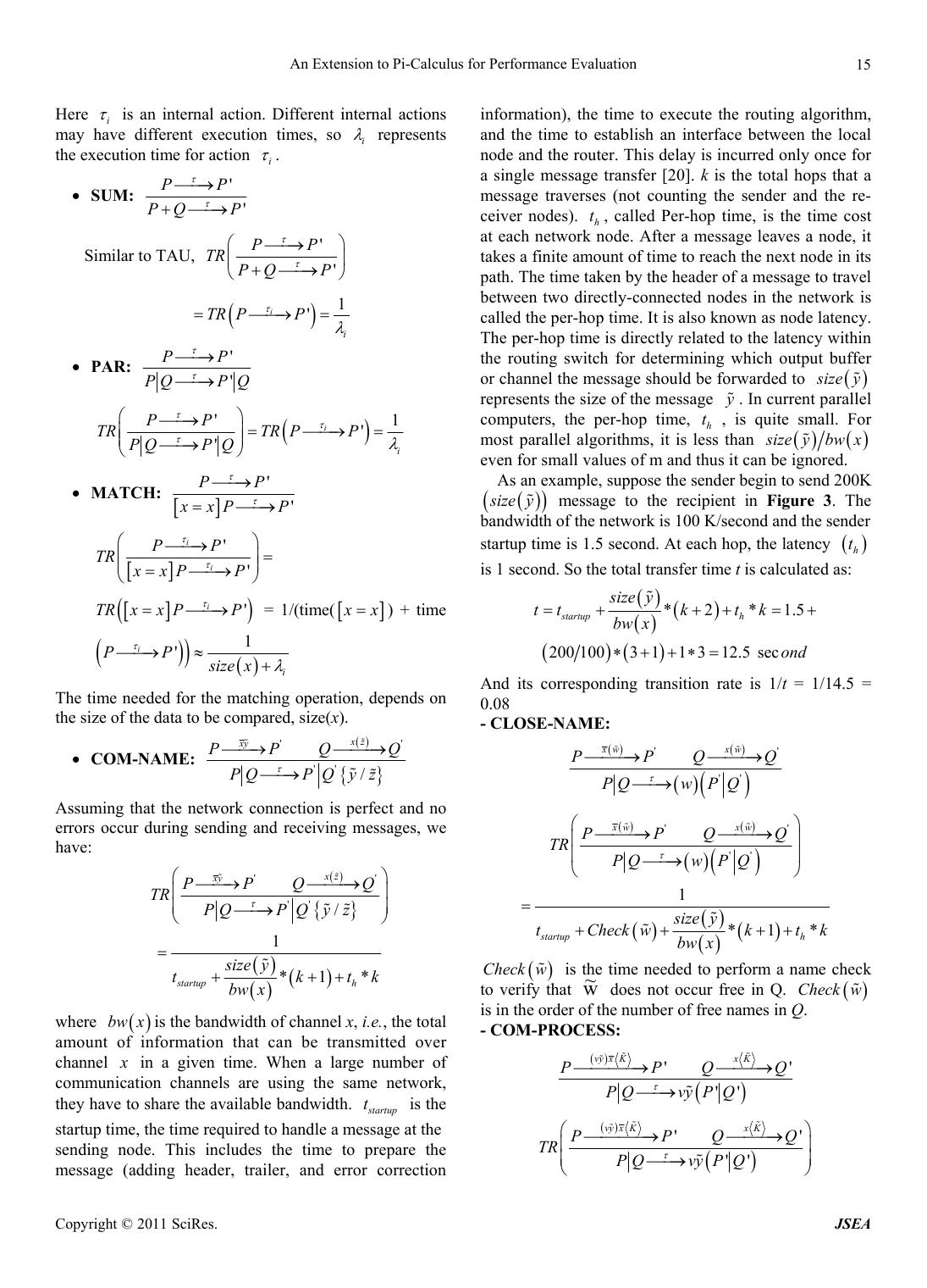











An Extension to Pi-Calculus for Perf orm anc e E valuation

Here i



is an internal action. Different internal actions

may have different execution times, so i



represents

the execution time for action i



 SUM: '

PQ P







Similar to TAU, '

TR PQP















TR PP







 PAR: '

PQP Q







TRTR PP

PQP Q

















 MATCH:



xP P









TR xxP P



















TRxx PP



 = 1/(time(





x) + time





size x









The time needed for the matching operation, depends on

the size of the data to be compared, size(x).

 COM-NAME:





'' /

PPQQ

PQPQyz











Assuming that the network connection is perfect and no

errors occur during sending and receiving messages, we

have:





'' /

PPQQ

TR PQPQyz



















 

*1 *

startup h

size y

tktk

bw x







where



bw xis the bandwidth of channel x, i.e., the total

amount of information that can be transmitted over

channel

in a given time. When a large number of

communication channels are using the same network,

they have to share the available bandwidth.

tartup

t is the

startup time, the time required to handle a message at the

sending node. This includes the time to prepare the

message (adding header, trailer, and error correction

information), the time to execute the routing algorithm,

and the time to establish an interface between the local

node and the router. This delay is incurred only once for

a single message transfer [20]. k is the total hops that a

message traverses (not counting the sender and the re-

ceiver nodes). h

t, called Per-hop time, is the time cost

at each network node. After a message leaves a node, it

takes a finite amount of time to reach the next node in its

path. Th e time ta k en b y th e hea d er o f a me ss a ge to tr av el

between two directly-connected nodes in the network is

called the per-hop time. It is also known as node latency.

The per-hop time is directly related to the latency within

the routing switch for determining which output buffer

or channel the message should be forwarded to





ize y



repre sents th e size of the me ssage

. In current parallel

computers, the per-hop time, h

t , is quite small. For

most parallel algorithms, it is less than









izeybw x



even for small values of m and thus it can be ignored.

As an example, suppose the sender begin to send 200K









ize y

 message to the recipient in Figure 3. The

bandwidth of the netwo rk is 100 K/second and the sender

startup time is 1.5 second. At each hop, the latency





is 1 second. So the total transfer time t is calculated as:





 

*2*1.5

startup h

size y

ttk tk

bw x















200100311312.5 sec ond

And its corresponding transition rate is 1/t = 1/14.5 =

0.08

- CLOSE-NAME:







xw xw

PPQQ

PQwPQ









 



xw xw

PPQQ

TR PQwP Q















 

*1 *

startup h

size y

tCheck wktk

bw x



 







Check w

 is the time needed to perform a name check

to verify that w

does not occur free in Q.





Check w



is in the order of the number of free names in Q.

- COM-PROCESS:



vy xKx K

PPQQ

PQvyP Q













vy xKx K

PPQQ

TR PQvy P Q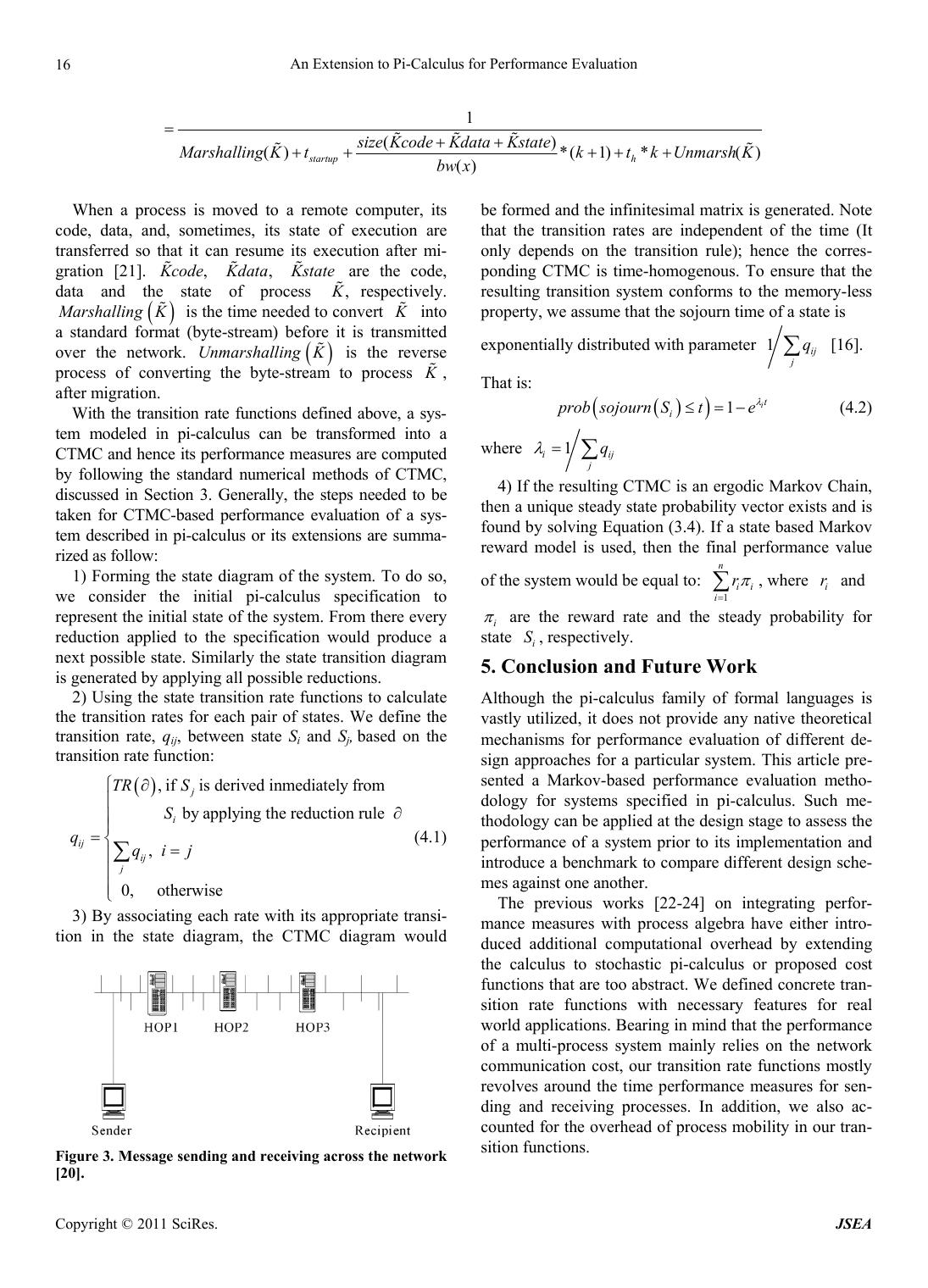

















An Extension to Pi-Calculus for Perf orm anc e E valuation

()

()*(1)*()

()

startup h

size KcodeKdataKstate

arshallingKtktkUnmarsh K

bw x



 





When a process is moved to a remote computer, its

code, data, and, sometimes, its state of execution are

transferred so that it can resume its execution after mi-

gration [21]. ,

cod e

 ,

data



state

 are the code,

data and the state of process ,

respectively.



arshalling K

 is the time needed to convert

 into

a standard format (byte-stream) before it is transmitted

over the network.



UnmarshallingK

 is the reverse

process of converting the byte-stream to process

,

after migration.

With the transition rate functions defined above, a sys-

tem modeled in pi-calculus can be transformed into a

CTMC and hence its performance measures are computed

by following the standard numerical methods of CTMC,

discussed in Section 3. Generally, the steps needed to be

taken for CTMC-based performance evaluation of a sys-

tem described in pi-calculus or its extensions are summa-

rized as follow:

1) Forming the state diagram of the system. To do so,

we consider the initial pi-calculus specification to

represent the initial state of the system. From there every

reduction applied to the specification would produce a

next possible state. Similarly the state transition diagram

is generated by applying all possible reductions.

2) Using the state transition rate functions to calculate

the transition rates for each pair of states. We define the

transition rate, qij, between state Si and Sj, based on the

transition rate function:



,ifis derived inmediately from

y applying the reduction rule

0, otherwise

TR S

qqij















 (4.1)

3) By associating each rate with its appropriate transi-

tion in the state diagram, the CTMC diagram would

Figure 3. Message sending and receiving across the network

[20].

be formed and the infinitesimal matrix is generated. Note

that the transition rates are independent of the time (It

only depends on the transition rule); hence the corres-

ponding CTMC is time-homogenous. To ensure that the

resulting transition system conforms to the memory-less

property, we assume that the sojourn time of a state is

exponentially distributed with parameter 1ij

 [16].

That is:









1it

prob sojourn Ste



 (4.2)

where 1

iij







4) If the resulting CTMC is an ergodic Markov Chain,

then a unique steady state p robability vector exists and is

found by solving Equ ation (3.4). If a state based Markov

reward model is used, then the final performance value

of the system would be equal to: 1





, where i

r and



are the reward rate and the steady probability for

state i

S, respectively.

5. Conclusion and Future Work

Although the pi-calculus family of formal languages is

vastly utilized, it does not provide any native theoretical

mechanisms for performance evaluation of different de-

sign approaches for a particular system. This article pre-

sented a Markov-based performance evaluation metho-

dology for systems specified in pi-calculus. Such me-

thodology can be applied at the design stage to assess the

performance of a system prior to its implementation and

introduce a benchmark to compare different design sche-

mes against one another.

The previous works [22-24] on integrating perfor-

mance measures with process algebra have either intro-

duced additional computational overhead by extending

the calculus to stochastic pi-calculus or proposed cost

functions that are too abstract. We defined concrete tran-

sition rate functions with necessary features for real

world applications. Bearing in mind that the performance

of a multi-process system mainly relies on the network

communication cost, our transition rate functions mostly

revolves around the time performance measures for sen-

ding and receiving processes. In addition, we also ac-

counted for the overhead of process mobility in our tran-

sition functions.

An Extension to Pi-Calculus for Perf orm anc e E valuation

The future studies should mai nly focus on the scalability

of the methodology to large complex systems with huge

number of states and transition rates. Many approaches are

proposed in literature to address the problem of state ex-

plosion in Markov chains [25-27].The incorporation of

these approaches with the performance evaluation of pi-

calculus models remains as a future work.

REFERENCES

[1] R. Milner, J. Parrow and D. Walker, “A Calculus of Mo-

bile Processes—Part I and II,” LFCS Report 89-85, Uni-

versity of Edinburgh, Edinburgh, 1989.

[2] R. Milner, “Communicating and Mobile Systems: The



-Calculus,” Cambridge University Press, Cambridge,

1999.

[3] R. Milner, “The Polyadic Pi-Calculus: A Tutorial,” Tech-

nical Report ECSLFCS -91-180, Computer Science De-

partment, University of Edinburgh, Edinburgh, 1991.

[4] D. Sangiorgi, “The



-Calculus: A Theory of Mobile

Processes,” Cambridge University Press, Cambridge, 2001.

[5] D. Sangiorgi: “Expressing Mobility in Process Algebras:

First-Order and Higher-Order Paradigms,” Ph.D. Thesis,

University of Edinburgh, Edinburgh, 1993.

[6] C. Priami, “Stochastic



-Calculus,” Computer Journal,

Vol. 38, 1995, pp. 578-589. doi:10.1093/comjnl/38.7.578

[7] N. G

 tz, U. Herzog and M. Rettelbach, “TIPP-A Lan-

guage for Timed Processes and Performance Evaluation,”

Technical Report 4/92. IMMD VII, University of Erlan-

gen-Nurnberg, Erlangen, 1992.

[8] J. Hillston, “A Compositional Approach to Performance

Modelling,” Ph.D. Thesis, University of Edinburgh,

Edinburgh, 1994.

[9] M. Bernardo, L. Donatiello and R. Gorrieri, “MPA: A

Stochastic Process Algebra,” Technial Report UBLCS-

94-10, University of Bologna, Bologna, 1994.

[10] P. Buchholz, “On a Markovian Process Algebra,” Tech-

inal Report Informatik IV, University of Dortmund, Dort-

mund 1994.

[11] L. de Alfaro, “Stochastic Transition Systems,” Proceed-

ings of Ninth International Conference on Concurrency

Theory (CONCUR’98), Vol. 1477, 1998, pp. 423-438.

doi:10.1007/BFb0055639

[12] J. Markovski and E. P. de Vink, “Performance Evaluation

of Distributed Systems Based on a Discrete Real- and

Stochastic-Time Process Algebra,” Fundamenta Informa-

ticae, Vol. 95, No. 1, October 2009, pp. 157-186.

[13] A. Clark, S. Gilmore, J. Hillston and M. Tribastone,

“Stochastic Process Algebras,” SFM’07 Proceedings of

the 7th International Conference on Formal Methods for

Performance Evaluation, 2007, pp 132-179.

[14] P. R. D’Argenio and J. Katoen, “A Theory of Stochastic

Systems. Part II: Process Algebra,” Information and

Computation, Vol. 203, No. 1, November 2005, pp. 39-74.

doi:10.1016/j.ic.2005.07.002

[15] S. M. Ross, “Stochastic Processes,” 2nd Edition, Wiley,

New York, 1996.

[16] G. Bolch, S. Greiner, H. De Meer and K. S. Trivedi,

“Queuing Networks and Markov Chains: Modelling and

Performance Evaluation with Computer Science Applica-

tions,” Wiley, New York, 1998

[17] C. Nottegar, C. Priami and P. Degano, “Performance

Evaluation of Mobile Processes Via Abstract Machines,”

IEEE Transactions on Software Engineering, Vol. 27, No.

10, 2001, pp. 867-889. doi:10.1109/32.962559

[18] F. Logozzo, “Pi-Calculus as a Rapid Prototype Language

For Performance Evaluation,” Proceedings of the ICLP

2001 Workshop on Specification, Analysis and Validation

for Emerging Technologies in Computational Logic

(SAVE 2001), 2001.

[19] S. Rahimi, M. Cobb, D. Ali, M. Paprzycki and F. Petry,

“A Knowledge-Based Multi-Agent System for Geospatial

Data Conflation,” Journal of Geographic Information and

Decision Analysis, Vol. 6, No. 2, 2002, pp. 67-81.

[20] A. Grama, G. Karypis, V. Kumar and A Gupta, “An In-

troduction to Parallel Computing: Design and Analysis of

Algorithms,” 2nd Edition, Addison Wesley, Reading,

2003.

[21] W. R. Cockayne and M. Zyda, “Mobile Agents,” Man-

ning Publications Company, Greenwich, 1998.

[22] H. Samet, “The Design and Analysis of Spatial Data

Structures,” Addison-Wesley, Reading, 1989.

[23] S. Rahimi, “Using Api-Calculus for Formal Modeling of

SDIAgent: A Multi-Agent Distributed Geospatial Data

Integration,” Journal of Geographic Information and De-

cision Analysis, Vol. 7, No. 2, 2003, pp. 132-149.

[24] S. Rahimi, J. Bjursell, M. Paprzycki, M. Cobb and D. Ali,

“Performance Evaluation of SDIAGENT, a Multi-Agent

System for Distributed Fuzzy Geospatial Data Confla-

tion,” Information Sciences, Vol. 176, No. 9, 2006.

doi:10.1016/j.ins.2005.07.009

[25] S. Derisavi, P. Kemper and W. H. Sanders, “Symbolic

State-Space Exploration and Numerical Analysis of

State-Sharing Composed Models,” Linear Algebra and Its

Applications, Vol. 386, July 2004, pp. 137-166. doi:10.

1016/j.laa.2004.01.006

[26] S. Derisavi, H. Hermanns and W. H. Sanders, “Optimal

State-Space Lumping in Markov Chains,” Information

Processing Letters, Vol. 87, No. 6, 2003, pp. 309-315.

doi:10.1016/S0020-0190(03)00343-0

[27] P. Buchholz, “Efficient Computation of Equivalent and

Reduced Representations for Stochastic Automata,” In-

ternational Journal of Computer Systems Science & En-

gineering, Vol. 15, No. 2, March 2000, pp. 93-103.