Vol.5, No.9, 1047-1055 (2013) Natural Science
http://dx.doi.org/10.4236/ns.2013.59129
Analytical expressions of the concentrations of
substrate and product in enzyme inhibition process
Sankaranarayanan Muthukumar, Lakshmanan Rajendran
Department of Mathematics, The Madura College, Madurai, India;
Received 3 June 2013; revised 3 July 2013; accepted 10 July 2013
Copyright © 2013 Sankaranarayanan Muthukumar, Lakshmanan Rajendran. This is an open access article distributed under the Crea-
tive Commons Attribution License, which permits unrestricted use, distribution, and reproduction in any medium, provided the
original work is properly cited.
ABSTRACT
The initial and boundary value problem in en-
zyme reactions mechanism for inhabitation proc-
ess is discussed. Approximate analytical exp re s-
sions for the concentrations of substrate and
product are presented. Approximate analytical
solutions of non-linear reaction equations con-
taining non-linear terms related to enzymatic re-
action mechanism are solved using Homotopy
perturbation method. The relevant analytical ex-
pression for the substrate and product concen-
tration profiles is discussed in terms of dimen-
sionless reaction diffusion parameters α, β, γE,
and γS. Numerical solution is also obtained us-
ing Matlab program. Our analytical expression
compared with numerical estimation and good
agreement is noted.
Keywords: Initial and Boundary V a lue Problems;
Enzyme Kinetics; Non-Linear Re action Equations;
Homotopy Perturbation Method; Michael is-Menten
Kinetics
1. INTRODUCTION
Enzymes are catalysts and increase the speed of a
chemical reaction without themselves undergoing any
permanent chemical change [1-7]. They are neither used
up in the reaction nor do they appear as reaction products.
An enzyme enhances the rate of the reaction it influences.
The catalysts is not consumed as a result of the reaction,
nor does it alter the equilibrium constant [8,9]. In this
two-step reaction, the enzyme combines with substrate to
form the complex, which can either dissociate again into
unchanged substrate and enzyme or go on to the second
step and form the products and unchanged enzyme. The
reverse of the second step would lead to the synthesis of
ES from enzyme and products, but this process can gen-
erally be ignored unless the products are allowed to ac-
cumulate. Also that the total substrate and product con-
centration in the enzyme kinetics in biochemical systems
has been modeled by system of nonlinear ordinary dif-
ferential equations.
An enzyme inhibitor is a molecule, which binds to
enzymes and decreases their activity. Since blocking an
enzyme’s activity can kill a pathogen or correct a meta-
bolic imbalance, many drugs are enzyme inhibitors. Th ey
are also used as herbicides and pesticides. Not all mole-
cules that bind to enzymes are inhibitors; enzyme acti-
vators bind to enzymes and increase their enzymatic ac-
tivity, while enzyme substrates bind and are conv erted to
products in the normal catalytic cycle of the enzyme.
The binding of an inhibitor can stop a substrate from
entering the enzyme’s active site. Inhibitor binding is ei-
ther reversible or irreversible. Irreversible inhibitors usu-
ally react with the enzyme and change it chemically. In
contrast, reversible inhibitors bind non-covalently and dif-
ferent types of inhibition are produced depending on
whether these inhibitors bind to the enzyme, the enzyme-
substrate complex, or both. Many drug molecules are en-
zyme inhibitors, so their discovery and improvement is
an active area of research in biochemistry and pharma-
cology.
Mathematical modeling of enzyme kinetics is given in
the books by Rubinow [10], Murray [11], Segel [12] and
Roberts [13]. Recently Rajendran and his team also solved
some non linear problems in enzyme reaction kinetics
[14-19]. The purpose of this communication is to derive
asymptotic approximate expressions for the concentra-
tion of substrate and product in enzyme inhibition proc-
ess.
2. MATHEMATICAL FORMULATION AND
ANALYSIS OF THE SUBSTRATE
INHIBITION MODELS
The sub strate act as an inh ibitor for enh ancing the ra te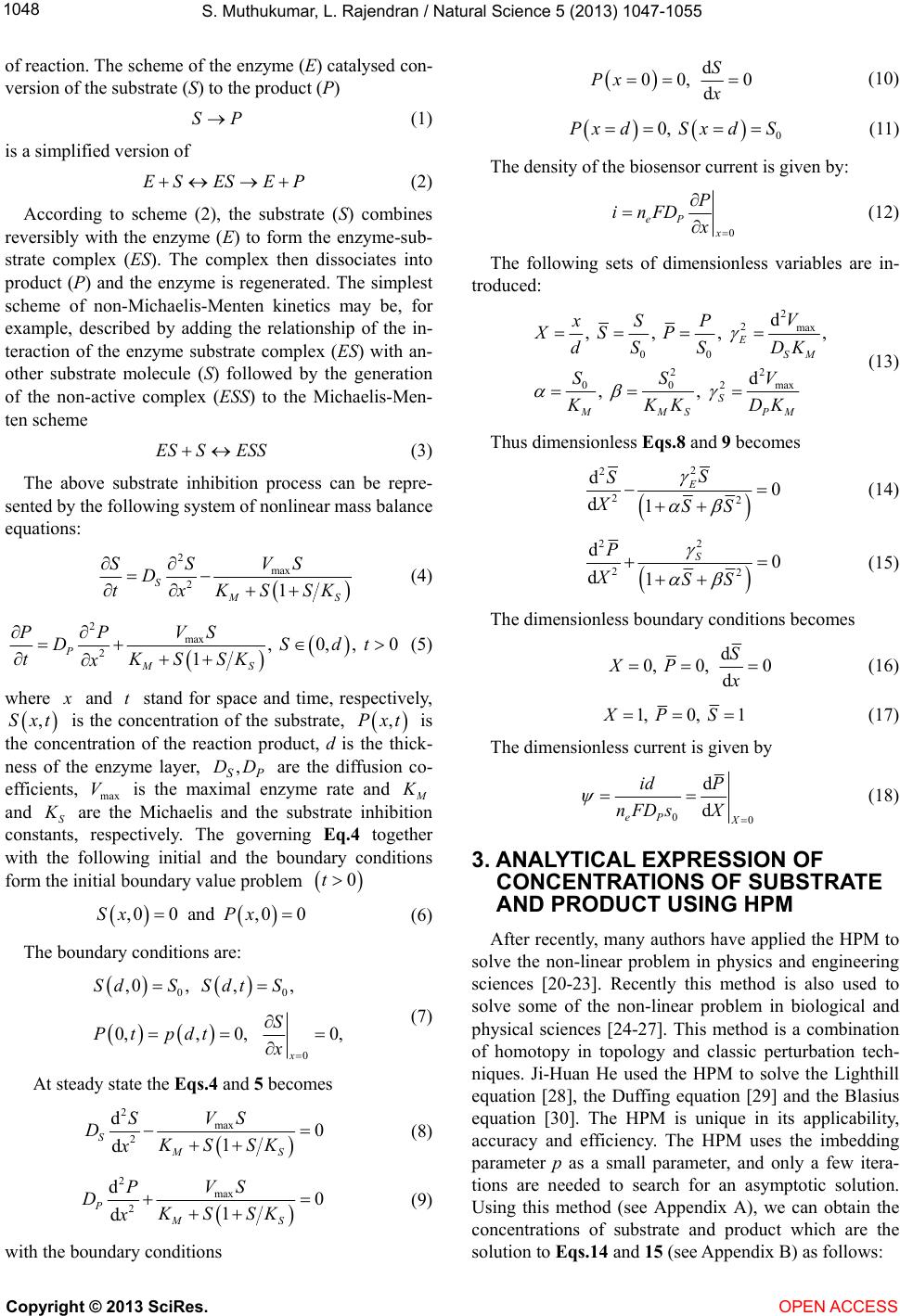

S. Muthukumar, L. Rajendran / Natural Science 5 (2013) 1047-1055
1048
of reaction. The scheme of the enzyme (E) catalysed con-
version of the substrate (S) to the product (P)
SP (1)
is a simplified version of
ESES EP  (2)
According to scheme (2), the substrate (S) combines
reversibly with the enzyme (E) to form the enzyme-sub-
strate complex (ES). The complex then dissociates into
product (P) and the enzyme is regenerated. The simplest
scheme of non-Michaelis-Menten kinetics may be, for
example, described by adding the relationship of the in-
teraction of the enzyme substrate complex (ES) with an-
other substrate molecule (S) followed by the generation
of the non-active complex (ESS) to the Michaelis-Men-
ten scheme
ES SESS (3)
The above substrate inhibition process can be repre-
sented by the f oll owi ng sy st em of nonli near m a ss bala nce
equations:

2max
21
S
M
S
VS
SS
D
tKSS x


 K
(4)


2max
2, 0,, 0
1
P
MS
VS PP
DS
tKSSK
x

 

dt
(5)
where
x
and stand for space and time, respectively, t


,Sxt is the concentration of the substrate,


,
P
xt is
the concentration of the reaction product, d is the thick-
ness of the enzyme layer, PS are the diffusion co-
efficients, max is the maximal enzyme rate and
DD ,
V
M
K
and S
K
are the Michaelis and the substrate inhibition
constants, respectively. The governing Eq.4 together
with the following initial and the boundary conditions
form the initial boundary value problem

0t



,00 and ,00Sx Px (6)
The boundary conditions are:
 
 
00
0
,0, ,,
0,,0, 0,
x
SdS SdtS
S
Pt pdtx


 

(7)
At steady state the Eqs.4 and 5 becomes

2max
2
d0
1 d
S
MS
VS
S
DKSSK
x  (8)

2max
2
d0
1 d
P
MS
VS
P
DKS SK
x  (9)
with the boundar y conditions

d
00, 0
d
S
Px x


(10)




0
0,
P
xdSxd S

 (11)
The density of the biosensor current is given by:
0
eP
x
P
inFD x

 (12)
The following sets of dimensionless variables are in-
troduced:
2
2max
00
22
2 00 max
d
, , , ,
d
, ,
E
SM
S
MMS PM
V xS P
XS P
dS SDK
SS V
KKK DK

 
 
 
(13)
Thus dimensi onl ess Eqs.8 and 9 becomes

2 2
22
d0
d1
ES
S
XSS




 (14)

2
2
22
d0
d1
S
P
XSS




 (15)
The dimensionless boundary conditions becomes
d
0, 0, 0
d
S
XP x

 (16)
1, 0, 1XPS

 (17)
The dim e ns i onless current is given by
00
d
d
eP X
id P
nFDs X


 (18)
3. ANALYTICAL EXPRESSION OF
CONCENTRATIONS OF SUBSTRATE
AND PRODUCT USING HPM
After recently, many authors have applied the HPM to
solve the non-linear problem in physics and engineering
sciences [20-23]. Recently this method is also used to
solve some of the non-linear problem in biological and
physical sciences [24-27]. This method is a combination
of homotopy in topology and classic perturbation tech-
niques. Ji-Huan He used the HPM to solve the Lighthill
equation [28], the Duffing equation [29] and the Blasius
equation [30]. The HPM is unique in its applicability,
accuracy and efficiency. The HPM uses the imbedding
parameter p as a small parameter, and only a few itera-
tions are needed to search for an asymptotic solution.
Using this method (see Appendix A), we can obtain the
concentrations of substrate and product which are the
solution to Eqs.14 an d 15 (see Appendix B) as follows:

S. Muthukumar, L. Rajendran / Natural Science 5 (2013) 1047-1055 104 9



22
1
22 2
273
4
222
sech sech
sech cosh
sinh cosh 2
cosh3
SS
SX
kNMNM
2
M
MX
N
kX MXkk MX
kMX
NNNN



 



(19)
 

 
275
2
65 12
223 22
64
22
2
2 57 6 12
2232
53 222
sech1
24
321cosh
48
1cosh2 1cosh3
36 9
3 2
sech
42 4
sinh
cosh 84
NM kk
PX M
kk
kk
M
MMM MM
kk
M
MM
kk k
kk N
XM
MMMM
kk
kX MX
MX MM

 

 


 





 




 





3
4
k
MX






2
6 424
22 322
2
636
22 22
cosh 2
2
cosh3
936 98
3sech
4436
MX
M
k kkk
MX 5
1
2
k
k
M
MMMM
kkk NM
MM MM




 



 

M
(20)
where 2
2,
1
E
M


 and


23
12
22 3
2
22 22
32
22
224 4
3
222
2222 2
222
22 4
2
45
22
sech tanh
2
sechcosh 2
6
3
sechcosh3sech tanh
32 8
sechsech sech
2
3
sechsech ,
28
sech, s
32
E
E
EE
ESS
EE
ES
NM
kMM
NM MM
NM NM
M
Mm
NMN N
MMM
NM NM
kM
NM N
kMk

















 

M
M
2
422
22
67
22
22
32
ech,
sech ,sech ,
2
sech,
6
SE
E
M
NNM
kMk M
NM
kM






(21)
The analytical expression of dimensionless current us-
ing the Eq.17 is given by

 

26
12
222
53
22
67 4
22
32
sech 14
1cosh 1cosh2
84
1cosh3 24
36 9
k
kk NM
MMM
kk
3
5
M
M
M
MM
kk kM
MM


 






 
 
 
 
k



(22)
4. NUMERICAL SIMULATION
The nonlinear differential Eqs.19 and 20 are also solved
by using numerical methods. The function ode45 in Mat-
lab software which is a function of solving two-point
boundary value problems (BVPs) for ordinary different-
tial equations is used to solve those equations. Its nu-
merical solution is compared with the solution obtained
by using Homotopy perturbation method and it gives a
satisfactory result. The Matlab program is also given in
Appendix C.
5. DISCUSSION
Eqs.19 and 20 are the new and simple analytical ex-
pressions of concentrations of the substrate and the prod-
uct calculated using Homotopy perturbation method. The
dimensionless analytical expressions of concentration
substrate


SX andproduct


P
X versus the di-
mensionless distance for various values of dimen-
sionless reaction parameters are compared with numeri-
cal solution in Figures 1 and 2.
X
From these figures, it is inferred that the value of the
concentration of substrate increases gradually when
increases. Also the concentration of substrate increases
when
X
E

decreases and

decreases. The concentra-
tion of substrate is uniform when 0.1
E

. From the
Figure 2, it is inferred that the product have minimum
value at 0X

and 1X

. Also it is maximum at X =
0.5. Concentration of product increases when the pa-
rameter
E

increases. Dimensionless current

ver-
sus dimensionless parameters ,, and
E
S
 
is plot-
ted in Figure 3. From these figure it is inferred that the
current increases when and

decreases or γE and γS
increases.
6. CONCLUSION
The analytical expressions for the concentration of
substrate and product in substrate inhibition process are
derived using new Homotopy perturbation method. We
have also presented an analytical expression for the s te a d y-
state current. The extension of procedure to various inhi-
bition models for steady-state and non-steady state con-
ditions seems possible. These analytical results will be
useful for the optimization and the design of enzyme
inhibition process.

S. Muthukumar, L. Rajendran / Natural Science 5 (2013) 1047-1055
1050
Figure 1. Plots of dimensionless concentration of substrate S(X) versus dimensionless distance X
for various values of parameter γE using Eq.19. The key to the plot: (•••) represents Eq.19 and (—)
represents numerical simulation.
Figure 2. Plots of dimensionless concentration of product P(X) versus dimensionless distance X
for various values of parameters γS using Eq.20. The key to the plot: (•••) represents Eq.20 and
(—) represents numerical simulation.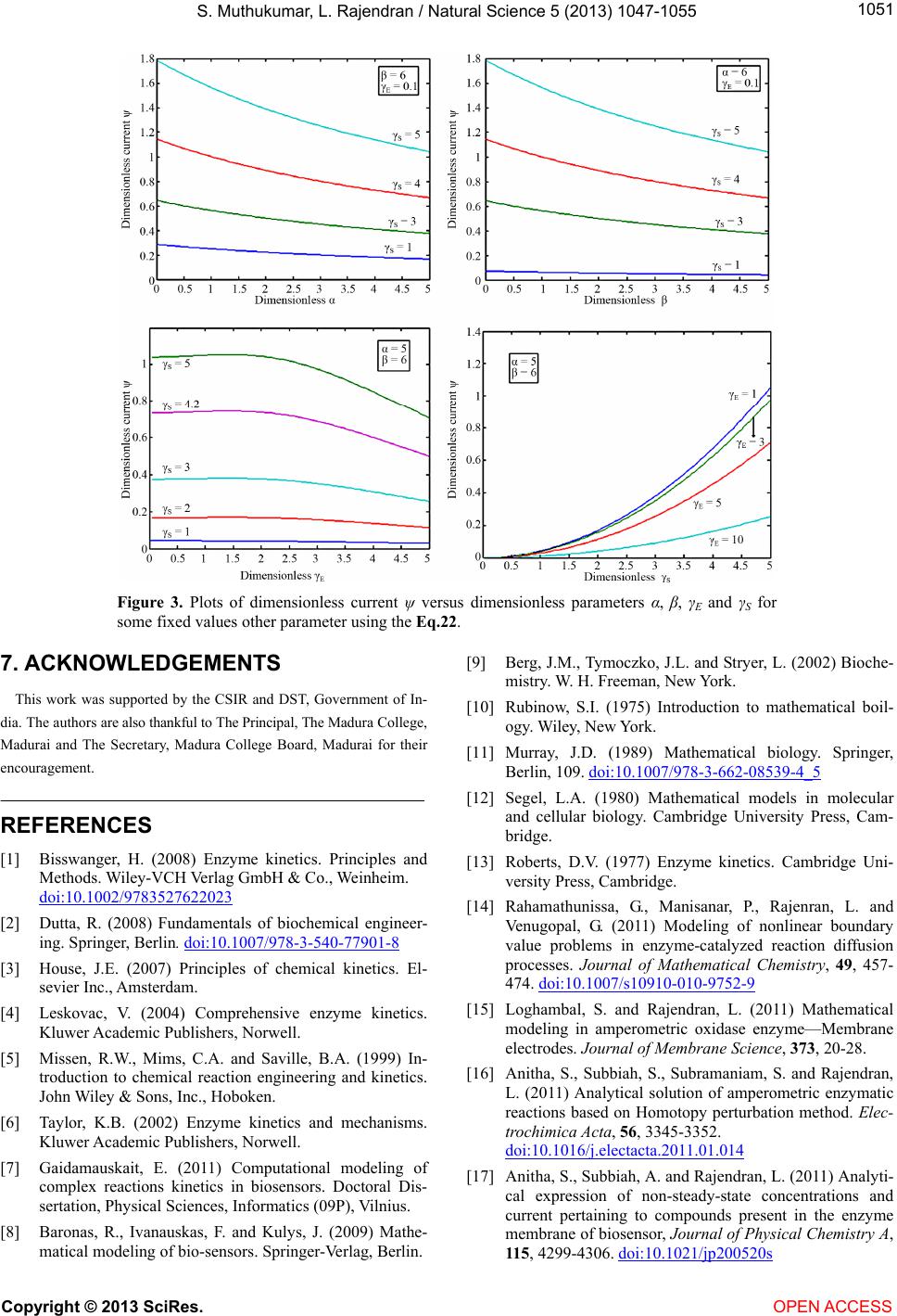

S. Muthukumar, L. Rajendran / Natural Science 5 (2013) 1047-1055 1051
Figure 3. Plots of dimensionless current ψ versus dimensionless parameters α, β, γE and γS for
some fixed values other parameter using the Eq.22.
7. ACKNOWLEDGEMENTS
This work was supported by the CSIR and DST, Government of In-
dia. The authors are also thankful to The Principal, The Madura College,
Madurai and The Secretary, Madura College Board, Madurai for their
encouragement.
REFERENCES
[1] Bisswanger, H. (2008) Enzyme kinetics. Principles and
Methods. Wiley-VCH Ve rlag GmbH & Co., Weinheim.
doi:10.1002/9783527622023
[2] Dutta, R. (2008) Fundamentals of biochemical engineer-
ing. Springer, Berlin. doi:10.1007/978-3-540-77901-8
[3] House, J.E. (2007) Principles of chemical kinetics. El-
sevier Inc., Amsterdam.
[4] Leskovac, V. (2004) Comprehensive enzyme kinetics.
Kluwer Academic Publishers, Norwell.
[5] Missen, R.W., Mims, C.A. and Saville, B.A. (1999) In-
troduction to chemical reaction engineering and kinetics.
John Wiley & Sons, Inc., Hoboken.
[6] Taylor, K.B. (2002) Enzyme kinetics and mechanisms.
Kluwer Academic Publishers, Norwell.
[7] Gaidamauskait, E. (2011) Computational modeling of
complex reactions kinetics in biosensors. Doctoral Dis-
sertation, Physical Sciences, Informatics (09P), Vilnius.
[8] Baronas, R., Ivanauskas, F. and Kulys, J. (2009) Mathe-
matical modeling of bio-sensors. Springer-Verlag, Berlin.
[9] Berg, J.M., Tymoczko, J.L. and Stryer, L. (2002) Bioche-
mistry. W. H. Freeman, New York.
[10] Rubinow, S.I. (1975) Introduction to mathematical boil-
ogy. W iley, New York.
[11] Murray, J.D. (1989) Mathematical biology. Springer,
Berlin, 109. doi:10.1007/978-3-662-08539-4_5
[12] Segel, L.A. (1980) Mathematical models in molecular
and cellular biology. Cambridge University Press, Cam-
bridge.
[13] Roberts, D.V. (1977) Enzyme kinetics. Cambridge Uni-
versity Press, Cambridge.
[14] Rahamathunissa, G., Manisanar, P., Rajenran, L. and
Venugopal, G. (2011) Modeling of nonlinear boundary
value problems in enzyme-catalyzed reaction diffusion
processes. Journal of Mathematical Chemistry, 49, 457-
474. doi:10.1007/s10910-010-9752-9
[15] Loghambal, S. and Rajendran, L. (2011) Mathematical
modeling in amperometric oxidase enzyme—Membrane
electrodes. Journal of Membrane Science, 373, 20-28.
[16] Anitha, S., Subbiah, S., Subramaniam, S. and Rajendran,
L. (2011) Analytical solution of amperometric enzymatic
reactions based on Homotopy perturbation method. Elec-
trochimica Acta, 56, 3345-3352.
doi:10.1016/j.electacta.2011.01.014
[17] Anitha, S., Subbiah, A. and Rajendran, L. (2011) Analyti-
cal expression of non-steady-state concentrations and
current pertaining to compounds present in the enzyme
membrane of biosensor, Journal of Physical Chemistry A,
115, 4299-4306. doi:10.1021/jp200520s

S. Muthukumar, L. Rajendran / Natural Science 5 (2013) 1047-1055
1052
[18] Uma Maheswari, M. and Rajendran, L. (2011) Analytical
solution of non-linear enzyme reaction equations arising
in mathematical chemistry. Journal of Mathematical Che-
mistry, 49, 1713-1726. doi:10.1007/s10910-011-9853-0
[19] Meena, A., Eswari, A. and Rajendran, L. (2011) Mathe-
matical modeling of biosensors: Enzyme-substrate Inter-
action and bio-molecular interaction. In: Serra, P.A., Ed.,
New Perspectives in Biosensors Technology and Applica-
tions, InTech, Rijeka. doi:10.5772/19513
[20] Ghori, Q.K., Ahmed, M. and Siddiqui, A.M. (2007) Ap-
plication of homotopy perturbation method to squeezing
flow of a Newtonian fluid. International Journal of Non-
linear Sciences and Numerical Simulation, 8, 179-184.
[21] Ozis, T. and Yildirim, A. (2007) A comparative study of
He’s homotopy perturbation method for determining fre-
quency-amplitude relation of a nonlinear oscillator with
discontinuities. International Journal of Nonlinear Sci-
ences and Numerical Simulation, 8, 243-248.
[22] Li, S.J. and Liu, Y.X. (2006) An improved approach to
nonlinear dynamical system identification using PID
neural networks. International Journal of Nonlinear Sci-
ences and Numerical Simulation, 7, 177-182.
doi:10.1515/IJNSNS.2006.7.2.177
[23] Mousa, M.M., Ragab, S.F. and Nturforsch, Z. (2008) Ap-
plication of the Homotopy perturbation method to linear
and nonlinear Schrödinger equations. Zeitschrift für Na-
turforschung, 63, 140-144.
[24] Margret PonRani, V. and Rajendran, L. (2010) Analytical
expression of non steady-state concentration profiles at
planar electrode for the CE mechanism. Natural Science,
2, 1318-1325. doi:10.4236/ns.2010.211160
[25] Varadharajan, G. and Rajendran, L. (2011) Analytical
solution of coupled non-linear second order reaction dif-
ferential equations in enzyme kinetics. Natural Science, 3,
459-465. doi:10.4236/ns.2011.36063
[26] Venugopal, K., Eswari, A. and Rajendran, L. (2011) Ma-
thematical model for steady state current at ppo-modified
micro-cylinder biosensors. Journal of Biomedical Science
and Engineering, 4, 631-641.
doi:10.4236/jbise.2011.49079
[27] Muthukumar, S. and Rajendran, L. (2012) Concentration
of species in two species oscillator using Homotophy
peturbation method. Global Journal of Theoretical and
Applied Mathematics Sciences, 2, 99-108.
[28] He, J.H. (1999) Homotopy perturbation technique. Com-
puter Methods in Applied Mechanics and Engineering,
178, 257-262.
[29] He, J.H. (2003) Homotopy perturbation method: A new
non-linear analytical technique. Applied Mathematics and
Computation, 135, 73-79.
doi:org/10.1016/S0096-3003(01)00312-5
[30] He, J.H. (2003) A simple perturbation approach to Blasius
equation. Applied Mathematics and Computation, 140,
217-222. doi:10.1016/S0096-3003(02)00189-3

S. Muthukumar, L. Rajendran / Natural Science 5 (2013) 1047-1055 1053
APPENDIX A: BASIC IDEA OF
HOMOTOPY PERTURBATION METHOD
In this appendix we outline the basic idea of Homo-
topy perturbation method. This method has eliminated
the limitations of the traditional perturbation methods.
On the other hand it can take full advantage of the tradi-
tional perturbation techniques, so there has been a con-
siderable deal of research in applying homotopy tech-
nique for solving various strongly nonlinear equations.
To explain Homotopy perturbation method, let us con-
sider the following function
 
0, Auf rr (A1)
with the boundary conditions,

,0, Bu unr  (A2)
where A, B,

f
r and  denote a general differential
operator, a boundary operator, a known analytical func-
tion and the boundary of the domain , respectively.
Generally speaking, the operator A can be divided into a
linear part L and a nonlinear part N. Eq.A1 can there fo re,
be written as

 


0LuNuf r (A3)
By Homotopy technique, we construct a Homotopy
 

,: 0,1vrp R which satisfies
  


0
,1
0.
0,1,
Hvpp LvLu
pAv fr
pr

  


 


(A4)
or
  

0
,
0.
0
H
vpLv LupLu
pNv fr
 
 

(A5)
where


0,1 p

0f r
is an embedding parameter, and μ0 is
an initial approximation of Eq.A1, which satisfies the
boundary conditions. When Eqs.A4 and A5 be-
come a linear equation; when it become a non-
linear equation. So the changing process of p from zero
to unity is just that of changing to
. We can first use the embedding pa-
rameter p as a small parameter. Obviously, from Eqs.A4
and A5, we will have
0p
p1
 
00Lv Lu

Av


 
0
,0 0HvLvLu 
(A6)



,10 HvAvf r  (A7)
Assume that the solutions of Eqs.A4 and A5 can be
written as a power series in p
2
01 2
vvpv pv  (A8)
Setting results in the approximate solution of
Eq.A1:
1p
012
1
lim
p
uvvvv


 (A9)
The combination of the perturbation method and the
Homotopy method is called the HPM.
APPENDIX B: SOLUTION OF EQS.14
AND 15 USING HPM
To find the solution of Eq.13, the homotopy is con-
structed as follows:

222
2
222
22 2
22
22 2
ddd
1ddd
dd d0
dd d
E
E
SSS
BS
XXX
SS S
BSS S
XX X

 





 


(B1)
The approximate solution of e Eq.B1 is:
2
01 2
SS BSBS

  (B2)
Substituting Eqs.B2 in B1 results:











22
01 01
22
201 201
2
201 01
2
22
2
01 01
01
22
201
dd
1dd
d
d
d
d
dd
dd
0
E
E
SBSSBS
BXX
SBSSBS
X
SBS
BSBS
X
SBS SBS
SBS
XX
SBS





 















 












(B3)
Comparing the coefficients of the powers of B
222
02 000
0
222
ddd
:0
ddd
E
SSS
BS
XX X



(B4)
222
12 111
1
222
22 22
2
00 00
00
22 22
ddd
:ddd
dd dd
0
dd dd
E
SS S
BS
XXX
SS SS
SS
XX XX

 


 
(B5)
The initial approximations are as follows:
01
dd
0, 0,0
dd
SS
XxX

 (B6)
01
1, 1, 0XS S

 (B7)
Solving (B4) and (B5) with boundary conditions (B6)
and (B7) gives
0sech coshSMMX

(B8)
and

S. Muthukumar, L. Rajendran / Natural Science 5 (2013) 1047-1055
1054
22
1
122 2
3
2
22
67
22
sechsech cosh
sinh cosh3
cosh 2
SS
kNN
SMM
N
k
kXMX MX
NN
kk MX
NN








MX
(B9)

01
gives the Eq.19. To find the solu-
tion of Eq.15, the homotopy is constructed as follows:
SXS S

222
2
222
222
22
222
ddd
1ddd
dd d0
dd d
S
S
PPP
BS
XXX
PPP
BSSS
XX X

 





 



(B10)
The approximate solution of Eq.B10 is:
2
01 2
PPBPBP  (B11)
Substituting (B11) in (B9) results:













22
01 01
22
201 201
2
201 01
2
2
2
01 01
01
22
201
dd
1dd
d
d
d
d
d
dd
0
S
E
PBP PBP
BXX
PBP SBS
X
PBP
BSBS
X
PBP PBP
SBS
XX
SBS





















 












2
d
(B12)
Comparing the coefficients of the powers of B
222
0
000
0
222
ddd
:
ddd
S
PPP
B
XXX
 
2
0S (B13)
222
12
111
1
222
22 22
2
00 00
00
22 22
ddd
:ddd
dd dd
0
dd dd
S
PPP
B
XXX
PP PP
SS
XX XX

 

 
S

(B14)
The initial approximations are as follows
01
At 0,0,0XPP (B15)
01
At 1,0,1XP P (B16)
Solving (B13) and (B14) with boundary conditions
(B15) and (B16) gives
 
2
02sech coshsech1sech
N
PMMXMX
M




6 12
1223
53
22
67 4
22
2
57 6 12
23 2
53 2222
6 42
321cosh
4
1cosh2
84
1cosh3 24
36 9
3 2cosh
42 4
sinh cosh 2
84
93
k
kk
PM
MMM
kk M
MM
kk kMX
MM
kk k kk
XM
MMM
kk
kX MXMX
MMM
k k
M






 



 
 

 
 

 

 
 





5
k
X
5 24
232
2
636 12222 2
2
cosh3
69
3sec
4436
k
kk
MX 2
8
M
MMM
kkk kNhM
MMMMM





 

(B18)


0
PXP P
1

 gives the Eq.20.
APPENDIX C: MATLAB PROGRAM TO
FIND THE NUMERICAL SOLUTION OF
EQS.14 AND 15
functio n pdex3
m = 0 ;
x = linspace(0,1);
t = linspace(0,1000 00000);
sol = pdepe(m,@pdex4pd e,@pdex4ic,@pdex4bc,x ,t);
u1 = sol(:,:,1);
u2 = sol(:,:,2);
%------------------------------------------------------
figure
plot(x,u1(end,:))
title(“u1(x,t)”)
xlabel(“Distance x”)
ylabel(“u1(x,2)”)
%---------------------------------------------------------------
figure
plot(x,u2(end,:))
title(“u2(x, t)”)
xlabel(“Distance x”)
ylabel(“u2(x,2)”)
% ---------------------------------------------------------
function [c,f,s] = pdex4pde(x,t,u,DuDx)
c = [1;1];
f = [1;1].* DuDx;
a=0.1; b=0.1; r1=0.1; r2=10;
F1 = -r1^2 * u(1)/(1 + a*u(1) + b*u(1)^2);
F2 = r2^2 * u(1)/(1 + a*u(1) + b*u(1)^2);
M
(B17)
s = [F1; F2];
% ---------------------------------------------------------
function u0 = pde x 4ic ( x)

S. Muthukumar, L. Rajendran / Natural Science 5 (2013) 1047-1055
1055
u0 = [1;1];
% --------------------------------------------------------
function [pl,ql,pr,qr] = pdex4bc(xl,ul,xr,ur,t)
pl = [0; ul(2)-0] ;
ql = [1; 0];
pr = [ur(1)-1 ; ur(2)-0];
qr = [0; 0];
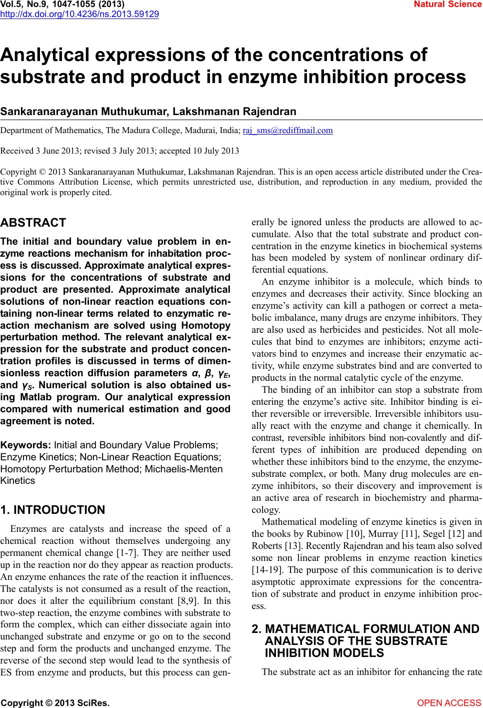