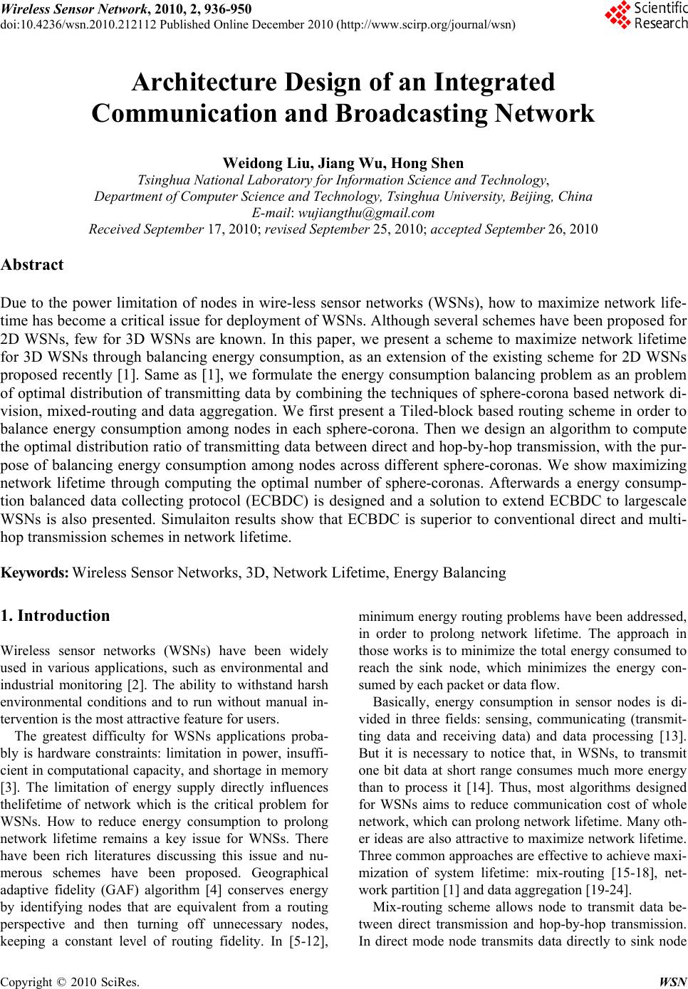Wireless Sensor Network, 2010, 2, 936-950
doi:10.4236/wsn.2010.212112 Published Online December 2010 (http://www.scirp.org/journal/wsn)
Architecture Design of an Integrated
Communication and Broadcasting Network
Weidong Liu, Jiang Wu, Hong Shen
Tsinghua National Laboratory for Information Scien ce and Technology,
Department of Com put er Science and Technology, Tsi n g hu a Universi t y, Beijing, Chin a
Received September 17, 2010; revised September 25, 2010; accepted September 26, 2010
Abstract
Due to the power limitation of nodes in wire-less sensor networks (WSNs), how to maximize network life-
time has become a critical issue for deployment of WSNs. Although several schemes have been proposed for
2D WSNs, few for 3D WSNs are known. In this paper, we present a scheme to maximize network lifetime
for 3D WSNs through balancing energy consumption, as an extension of the existing scheme for 2D WSNs
proposed recently [1]. Same as [1], we formulate the energy consumption balancing problem as an problem
of optimal distribution of transmitting data by combining the techniques of sphere-corona based network di-
vision, mixed-routing and data aggregation. We first present a Tiled-block based routing scheme in order to
balance energy consumption among nodes in each sphere-corona. Then we design an algorithm to compute
the optimal distribution ratio of transmitting data between direct and hop-by-hop transmission, with the pur-
pose of balancing energy consumption among nodes across different sphere-coronas. We show maximizing
network lifetime through computing the optimal number of sphere-coronas. Afterwards a energy consump-
tion balanced data collecting protocol (ECBDC) is designed and a solution to extend ECBDC to largescale
WSNs is also presented. Simulaiton results show that ECBDC is superior to conventional direct and multi-
hop transmission schemes in network lifetime.
Keywords: Wireless Sensor Networks, 3D, Network Lifetime, Energy Balancing
1. Introduction
Wireless sensor networks (WSNs) have been widely
used in various applications, such as environmental and
industrial monitoring [2]. The ability to withstand harsh
environmental conditions and to run without manual in-
tervention is the most attractive feature for users.
The greatest difficulty for WSNs applications proba-
bly is hardware constraints: limitation in power, insuffi-
cient in computational capacity, and shortage in memory
[3]. The limitation of energy supply directly influences
thelifetime of network which is the critical problem for
WSNs. How to reduce energy consumption to prolong
network lifetime remains a key issue for WNSs. There
have been rich literatures discussing this issue and nu-
merous schemes have been proposed. Geographical
adaptive fidelity (GAF) algorithm [4] conserves energy
by identifying nodes that are equivalent from a routing
perspective and then turning off unnecessary nodes,
keeping a constant level of routing fidelity. In [5-12],
minimum energy routing problems have been addressed,
in order to prolong network lifetime. The approach in
those works is to minimize the total energy consumed to
reach the sink node, which minimizes the energy con-
sumed by each packet or data flow.
Basically, energy consumption in sensor nodes is di-
vided in three fields: sensing, communicating (transmit-
ting data and receiving data) and data processing [13].
But it is necessary to notice that, in WSNs, to transmit
one bit data at short range consumes much more energy
than to process it [14]. Thus, most algorithms designed
for WSNs aims to reduce communication cost of whole
network, which can prolong network lifetime. Many oth-
er ideas are also attractive to maximize network lifetime.
Three common approaches are effective to achieve maxi-
mization of system lifetime: mix-routing [15-18], net-
work partition [1] and data aggregation [19-24].
Mix-routing scheme allows node to transmit data be-
tween direct transmission and hop-by-hop transmission.
In direct mode node transmits data directly to sink node

W. D. LIU ET AL. 937
while transmitting data to next hop node in hop-by-hop
mode. Energy consumption balance may be achieved if
node chooses an appropriate data allocation in these two
transmission modes, and then maximization of network
lifetime could be achieved accordingly.
Network partition has great influence on network life-
time. A good dividing method may reduce the amount of
data transmitted, save energy of sensor nodes, and then
prolong the system lifetime. Slice-based partition and
corona-based partition are two common methods for
network partition. Slice-based partition divide circular
network into slices. And Corona-based partition method
divides circular network area into coronas centred with
sink node with different radius.
Data aggregation is a useful technique to eliminate
redundant data of network. Nodes in small area are close
to each other and may generate redundant sensing data in
WSNs like temperature monitoring WSNs. In data ag-
gregation a node may pack its input data into a different
size outputted, reduce unnecessary data transmission and
save energy, which extends the lifetime of network.
For common situations, WSNs are mainly used in a
two dimensional environment. Recently there are emer-
ging applications deploying WSNs in a three dimension-
al environment, such as marine environment monitoring
and safety monitoring for coal mine that have attracted
interesting attention. Compared to 2D deployment, due
to the sufficient increase in the number of sensor nodes
within the coverage of WSNs in a 3D deployment, the
limit in power storage and supply remains even more
severe for WSNs in 3D applications. In this paper, we
present a method to maximize network lifetime by ba-
lancing the energy consumption at all nodes for 3D
WSNs deployment. The main contributions of this paper
can be summarized as follows:
• Similar to the zone based routing scheme in [1], we
propose a routing scheme called tiled-block routing for
3D environment. Our work is inspired and extends the
solution of [1] from 2D to 3D.
• Using a method similar to corona-partition, we pro-
pose a decomposing method that decomposes a 3D mon-
itoring sphere space into sphere-coronas, and then break
energy consumption balance down to two levels: intra
sphere-corona and inter sphere-corona.
• We propose a scheme to achieve intra energy con-
sumption balance, through partitioning each sphere co-
rona into a set of sphere subcoronas, such that data
transmission takes place only between two sphere sub-
coronas that have the same relative positions in two
neighbouring sphere-coronas.
• We propose a scheme to achieve inter energy con-
sumption balance, by computing a proper data distribu-
tion ratio for each sphere-corona between direct and
hop-by-hop transmission.
• We show that maximizing network lifetime can be
achieved through setting an optimal number of
sphere-coronas and that of sphere subcoronas within
each corona.
This paper is organized as follows: Section 2 presents
the system model and the statement of problems. Sec-
tions 3 and 4 give the solutions for the intra sphere coro-
na energy balance problem and inter sphere-corona
energy balance problem. Section 5 solves the maximiz-
ing network lifetime problem. Section 6 presents a pro-
tocol called ECBDC and Section 7 give the solutions to
extend ECBDC to large-scale sensor network. In Section
8, the ECBDC is evaluated through simulation and com-
pared to other protocols. And the conclusion of this pa-
per is given in Section 9.
2. System Models and Problem Statement
2.1. Network Model
We assume that all sensor nodes are distributed in a
sphere space S of radius R, in which the node distribu-
tion density is ρ. There is only one sink node that is lo-
cated at the core of S. All nodes have the same maximum
range of transmission Tmax that is larger than R and the
same amount of initial energy. Every node knows its
geographic location.
The data operation is divided into T rounds. In one
word, nodes receive data and generate data then transmit
it in one round. In the gap of two adjacent rounds, nodes
turn off its radio to save the energy.
2.2. Data Aggregation Model
We use a function [25] to illustrate the data aggregation
model:


x
mx c   (1)
where φ(x) is the amount of data output, x is the
amount of data received, m is the aggregation propor-
tion and c is a const that depends on specific situation:
• If m = 0 and c > 0, the amount of data that will be
transmitted in one node in one round is small so that it
can be put in a single packet.
• If m = 1 and c = 0, in this case, the node does not
perform any data aggregation.
• If 0 < m < 1 and c = 0, the node compresses the data
output by a factor of m.
2.3. Energy Model
The energy consumption function is given below:


k
elec amp
x
x 

 (2)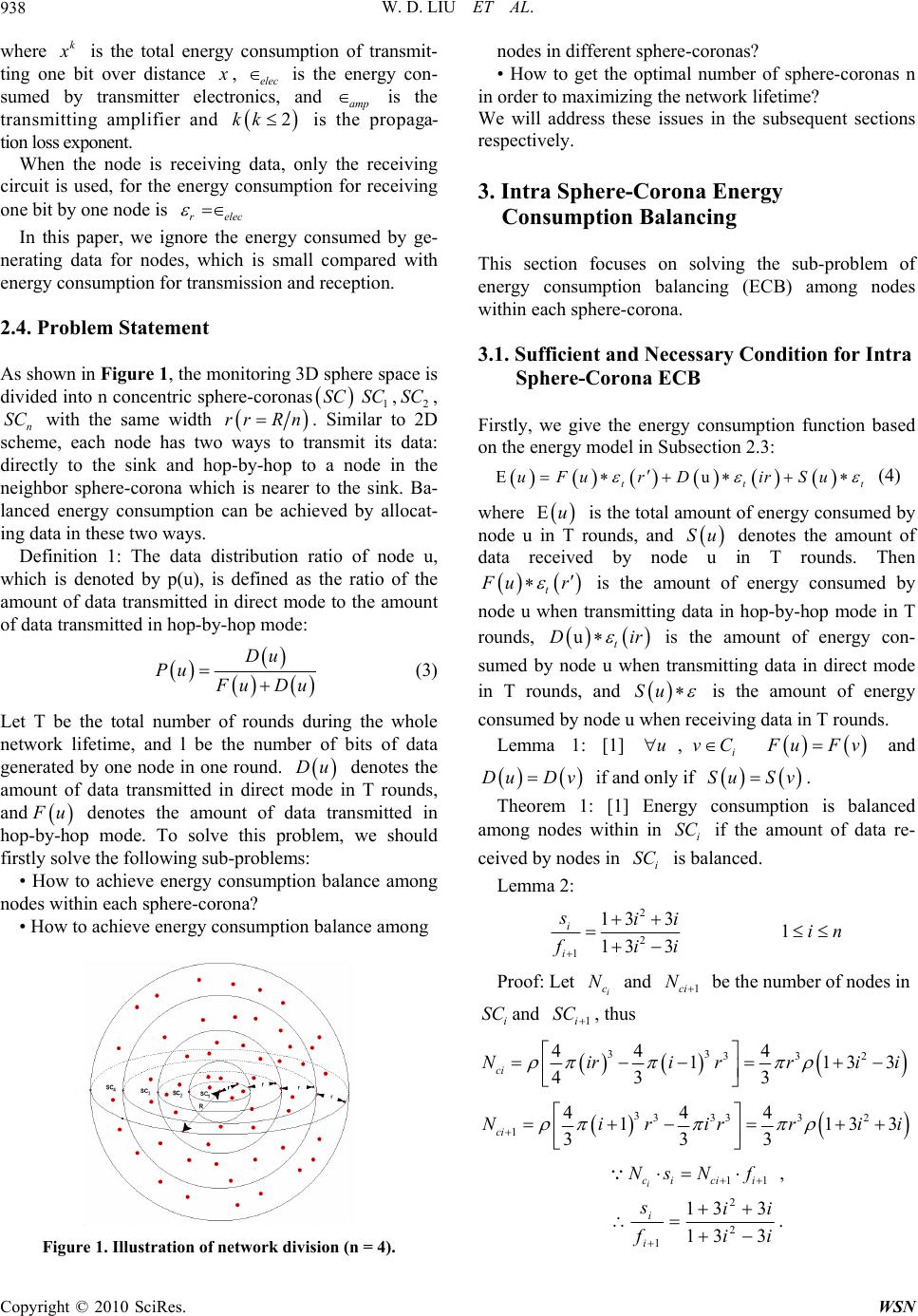

W. D. LIU ET AL. 938
where k
x
is the total energy consumption of transmit-
ting one bit over distance
x
, elec  is the energy con-
sumed by transmitter electronics, and amp  is the
transmitting amplifier and

2kk is the propaga-
tion loss exponent.
When the node is receiving data, only the receiving
circuit is used, for the energy consumption for receiving
one bit by one node is relec


In this paper, we ignore the energy consumed by ge-
nerating data for nodes, which is small compared with
energy consumption for transmission and reception.
2.4. Problem Statement
As shown in Figure 1, the monitoring 3D sphere space is
divided into n concentric sphere-coronas


SC 1 SC ,2 SC ,
n
SC with the same width


rr Rn. Similar to 2D
scheme, each node has two ways to transmit its data:
directly to the sink and hop-by-hop to a node in the
neighbor sphere-corona which is nearer to the sink. Ba-
lanced energy consumption can be achieved by allocat-
ing data in these two ways.
Definition 1: The data distribution ratio of node u,
which is denoted by p(u), is defined as the ratio of the
amount of data transmitted in direct mode to the amount
of data transmitted in hop-by-hop mode:
 
 
Du
Pu
F
uDu
 (3)
Let T be the total number of rounds during the whole
network lifetime, and l be the number of bits of data
generated by one node in one round.

Du denotes the
amount of data transmitted in direct mode in T rounds,
and

F
u denotes the amount of data transmitted in
hop-by-hop mode. To solve this problem, we should
firstly solve the following sub-problems:
• How to achieve energy consumption balance among
nodes within each sphere-corona?
• How to achieve energy consumption balance among
Figure 1. Illustration of network division (n = 4).
nodes in different sphere-coronas?
• How to get the optimal number of sphere-coronas n
in order to maximizing the network lifetime?
We will address these issues in the subsequent sections
respectively.
3. Intra Sphere-Corona Energy
Consumption Balancing
This section focuses on solving the sub-problem of
energy consumption balancing (ECB) among nodes
within each sphere-corona.
3.1. Sufficient and Necessary Condition for Intra
Sphere-Corona ECB
Firstly, we give the energy consumption function based
on the energy model in Subsection 2.3:












u
ttt
uFurDirSu




  
(4)
where


u is the total amount of energy consumed by
node u in T rounds, and

Su denotes the amount of
data received by node u in T rounds. Then




t
F
ur 

 is the amount of energy consumed by
node u when transmitting data in hop-by-hop mode in T
rounds,




ut Dir   is the amount of energy con-
sumed by node u when transmitting data in direct mode
in T rounds, and


Su


is the amount of energy
consumed by node u when receiving data in T rounds.
Lemma 1: [1] u

,i vC



F
uFv and




Du Dv if and only if




Su Sv.
Theorem 1: [1] Energy consumption is balanced
among nodes within in i
SC if the amount of data re-
ceived by nodes in i SC is balanced.
Lemma 2:
2
2
1
13 3
13 3
i
i
sii
fii





 1in
Proof: Let i
c
N and 1ci
N

be the number of nodes in
i
SC and 1i SC

, thus
 

33
332
44 4
1133
43 3
ci
Nirirrii  






33333 2
1
444
1133
333
ci
Nirirrii  





11
i
cici i
Ns Nf

 ,
2
2
1
13 3
13 3
i
i
sii
fii




.

W. D. LIU ET AL. 939
3.2. Tiled-block Based Routing Scheme
The basic idea of the Tiled-block (TB) is illustrated
as follows: As shown in Figure 2, each sphere-corona is
divided into

sphere subcoronas with equal width
rw, then the spherical surface of each sphere subcorona
is divided with latitudes of number a L and then longi-
tudes of number L
O, with a
L and L
O defined by
users. Moreover, the Lo longitudes divide the spherical
surface into L
O same cambered surfaces with equal
radian and equal width , and La latitudes divide each
longitude into 1
a
L equilength arcs. Nodes in sphere
subcorona SCi use two tuples to express their
Tiled-block ID

, ,eghk . Index h locates nodes in
latitudinal direction and index

locates nodes in lon-
gitudinal direction.
For any node

,,,
uuu
u

 denotes the three dimen-
sional polar coordinates of u, and ,,,ijhk TB denotes the tiled
block

,hk in,ij SC , i h and 1i h denote the distance
between plane
A
BCD and plane EFGH and the distance
between plane
I
JKL and plane
M
NOP respectively.
Figure 2. 1,,, TBijhkand ,,, TBijhkin a sphere space.
Lemma 3:


1
2
jr
ir
BC ABw
jr
IL IJir
w



Proof: As shown in Figure 2, let
B
C

be the radian
of

BC ,

R
B
C be the radius of spherical surface which

BC belongs to, and BC be the length of line whose two
endpoints are nodes B and C. Obviously,
A
DBC,
because

A
D and

BC belong to the same spherical
surface and the length of arc

A
D equals to the length
of arc

BC . With the same reason, EH FG,
J
KIL

, OP MN



=,
2sinR
2
=2sin1
2
BCIL ABIJ
BC BC
BC
BC
jr
ir
w




 










2sinR
2
=2sin2
2
1
2
IL IL
IL
IL
jr
ir
w
jr
ir
BC w
jr
IL ir
w


 










2sin R
2
=2sin1
2
AB AB
AB
AB
jr
ir
w


 





2sin R
2
IJ
I
J
IJ




=2 sin2
2
IJ jr
ir
w







1
2
jr
ir
A
BBC
w
jr
I
JIL
ir
w




Lemma 4
1
=2
ii
hh in

Proof: As shown in Figure 2,
== cos= cos
ir
hFSBFS BFBFSw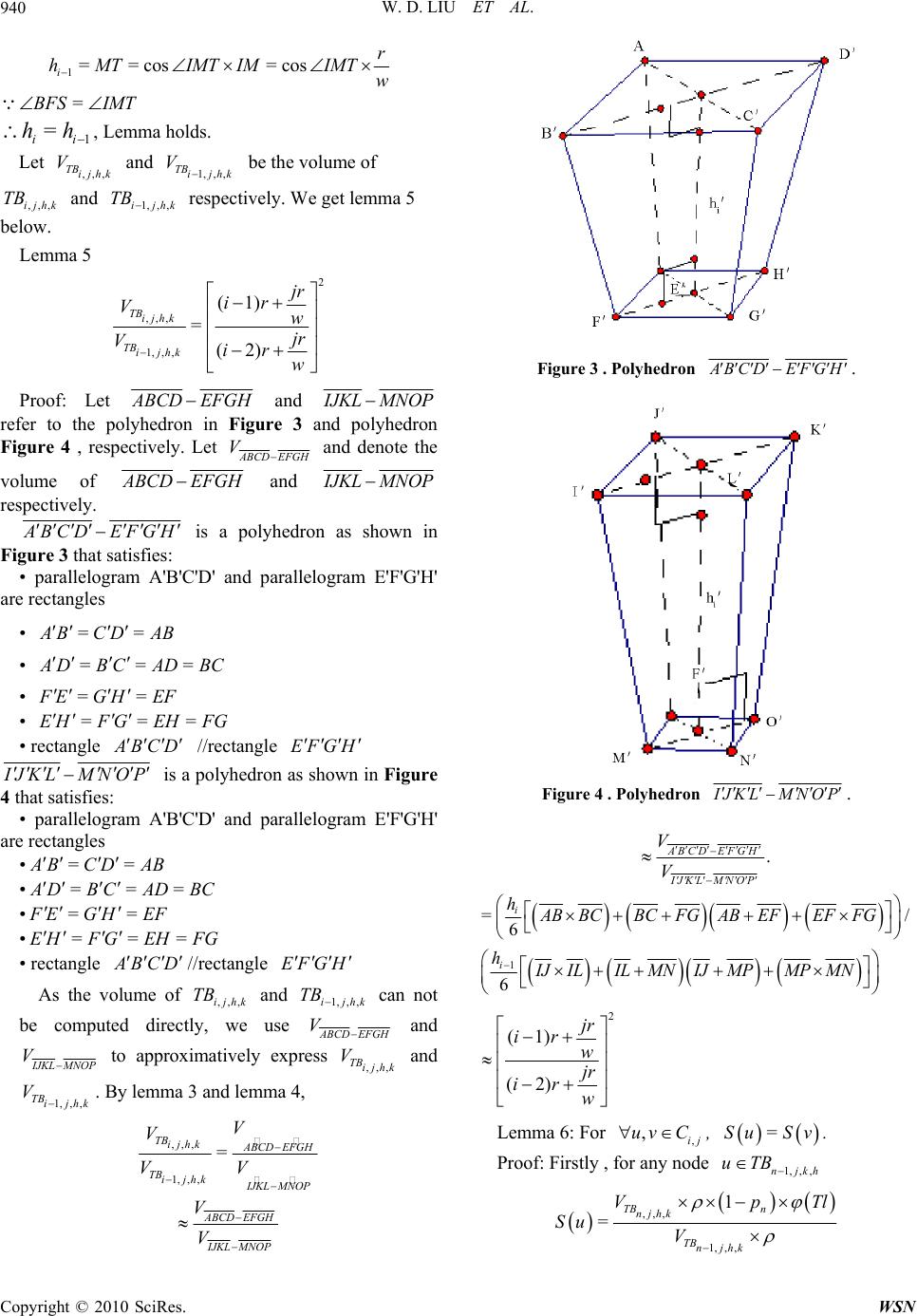



W. D. LIU ET AL. 940
1== cos= cos ir
hMTIMT IMIMTw
 
=BFS IMT
1
=

ii hh, Lemma holds.
Let ,,,
TBijhk
V and 1,,,
TBijhk
V be the volume of
,,,ijhk
TB and 1,, ,ijhk TB  respectively. We get lemma 5
below.
Lemma 5
2
,,,
1,,,
(1)
=
(2)
TBijhk
TBijhk
jr
ir
Vw
jr
Vir
w








Proof: Let
A
BCD EFGH and
I
JKL MNOP
refer to the polyhedron in Figure 3 and polyhedron
Figure 4 , respectively. Let ABCD EFGH V and denote the
volume of
A
BCD EFGH and
I
JKL MNOP
respectively.
A
BCD EFGH
 
 is a polyhedron as shown in
Figure 3 that satisfies:
• parallelogram A'B'C'D' and parallelogram E'F'G'H'
are rectangles
• ==
A
BCDAB
 
• ===
A
DBCADBC
 
• ==
F
EGHEF
 
• ===EHFGEH FG
 
• rectangle
A
BCD

//rectangle EFGH
 
I
JKL MNOP
   
 is a polyhedron as shown in Figure
4 that satisfies:
• parallelogram A'B'C'D' and parallelogram E'F'G'H'
are rectangles
•==
A
BCDAB
 
•===
A
DBCADBC
 
•==
F
EGHEF
 
•=== EHFGEH FG
 
• rectangle
A
BCD

//rectangle EFGH
 
As the volume of ,,,ijhk
TB and 1,, ,ijhk TB  can not
be computed directly, we use ABCD EFGH V and
I
JKL MNOP
V to approximatively express ,,,
TBijhk
V and
1,,,
TBijhk
V. By lemma 3 and lemma 4,
,,,
1, , ,
=
TBijhk ABCD EFGH
TBijhk
I
JKL MNOP
V
V
VV




ABCD EFGH
I
JKL MNOP
V
V



Figure 3 . Polyhedron
A
BCD EFGH
 
.
Figure 4 . Polyhedron IJKLMNOP
 
.
.
ABCD EFGH
IJKLMNOP
V
V

 


  



1
=/
6
6
i
i
hAB BCBCFGABEFEFFG
hIJILILMNIJMPMP MN




 






  



2
(1)
(2)
jr
ir
w
jr
ir
w













Lemma 6: For , ,ij uv C

,
 
=Su Sv.
Proof: Firstly , for any node 1, ,,njkh uTB



 
,,,
1, , ,
1
=TB n
njhk
TBnjhk
VpTl
Su V



 


W. D. LIU ET AL. 941
 
,,,
1, , ,
=1
TBnjhk n
TBnjhk
VpTl
V



By lemma 5
(1)
()=
(2)
jr
nr
w
Su jr
nr
w







,
we can see that

Su is a function of variable j, n p,
w, which are the same to for nodes in 1, , ,njhk TB .
Besides, n, T and l are constants. Therefore, for
any nodes u, v, ()= ()Su Sv. Secondly, suppose that
the amount of data received by any node in i SC is
balanced. For any node 1,,,ijhk uTB

,




,
,,,
1, , ,
1
=TBii j
ijhk
TBijhk
VpTlS
Su V



 



,,,
,
1, , ,
=1
TBijhk iij
TBijhk
VpTlS
V







2
,
1
=1
2
iij
j
ir
rw pTlS
j
ir
rw









So, the amount of data received by nodes in 1,ij SC  is
balanced.
Theorem 2 The amount of data received by nodes in
i
SC is balanced in Tiled-block based on routing scheme
if

2223
3
3
,223
133 33
=1
13
ij iiijijj
rri w
isiw w


 



Proof: By lemma 2,
2
1,1 1,21,
2
,1 ,2,
13 3
====
13 3
CC C
ii iw
CC C
ii iw
VVV ii
VVV ii
 





3
3
=1 1,
3
33
=1 ,,
44
33
=44
1
33
j
C
kik
j
C
kik ij
jr
ir ir
Vw
Vrir











2
2
13 3
=133
ii
ii



2223
3
3
,223
133 33
=1
13
ij iiijij j
rri w
isiww


 



4. Inter Sphere-Corona Energy Consump-
tion Balancing
This section focus on solving the sub-problem of
balancing energy consumption among nodes in different
sphere-coronas.
4.1. Hop-by-Hop Transmission Distance
In this section, we compute the hop-by-hop transmission
distance '
i
r for each sphere-corona i SC .
Theorem 3: Let * w be the optimal number of sphere
subcoronas for maximizing i
r, then,

2
2*
**
21 1
1
'1 2
i
iw
rr wiw




 







1
2
2
22
4sin sin
21
ao
i
LL










where *
=1,2,
=()
in
wmax hi
, function


=whi is
determined by equation below:


2
22
23
11
421
sin sin
221
ao
ri
LL ww









2
23
11
2=0rww




Proof: All nodes in i SC have the same hop-by-hop
transmission distance i r

. We assume that point Y and
point
Z
are two points located in the same sphere
subcorona and keep the same distance to sink. Obviously,
these two points are located on the same spherical
surface centered at the sink. Then let

YZ

be the radian
of

YZ , and

YZ
R be the radius of spherical surface to
which

YZ belongs.
As shown in Figure 5, obviously the hop-by-hop
transmission distance =
i
rAC

 , now we are going to
compute the length of
A
C

.What shown in Figure 6 is
the top view of tiled-block ,,,ijhk TB , and the profile of
arc

BC in Figure 7. Point O in (b) denotes the sink,
which is the core of the sphere space. We can get,


=2sin2
DC
D
C
DC R



=2sin21
a
OC
L





=2sin1
21
a
jr
ir
Lw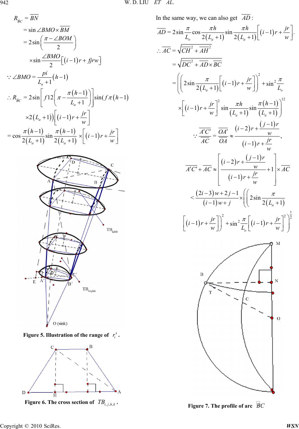










W. D. LIU ET AL. 942

=
BC
RBN
=sinBMO BM
=2sin2
BOM
 




sin 1
2
BMO irfjrw 
 


=1
1
a
pi
BMO h
L




 
1
=2sin 12sin(1
1
BC a
h
Rf fh
L




 









21 1
ajr
Lir
w

 






11
=cos sin
2121
aa
hh
LL
 


1jr ir
w




Figure 5. Illustration of the range of '
i
r.
Figure 6. The cross section of ,,,ijhk TB .
In the same way, we can also get
A
D:


=2sin cossin1.
2121
oa a
hh jr
ADi r
LL Lw
 





22
=
A
CCHAH
2
=DCAD BC


2
2
=2sin1sin
21
ao
jr
ir
LwL















12
21
1sin sin
11
aa
h
jr h
ir
wL L





 
 






1
2
=,
1
jr
ir
AC OAw
jr
AC OAir
w


 






1
2
1
1
jr
ir w
A
CAC AC
jr
ir
w




 







232 1
<2sin
121
a
iwj
iwj L










 
1
222
2
11
sin
o
jr jr
ir ir
wL w




 






Figure 7. The profile of arc

BC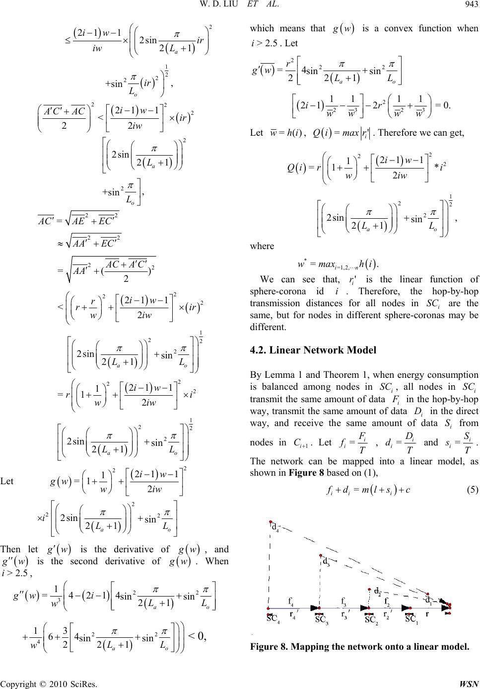

W. D. LIU ET AL. 943


2
211 2sin 21
a
iw ir
iw L











1
2
2
2,
sin
o
ir
L




 
22
2
21 1
<
22
iw
AC ACir
iw

  







2
2sin 21
a
L











2,
sin
o
L




22
=
A
CAEEC


22
A
AEC


22
=()
2
ACA C
AA 


 
2
2
2
21 1
<2
iw
r
rir
wiw


 






1
22
2
2sin sin
21
ao
LL




 














2
2
2
21 1
1
=1 2
iw
ri
wiw


 






1
22
2
2sin sin
21
ao
LL




 













Let
 
2
221 1
1
=1 2
iw
gw wiw












2
22
2sin sin
21
ao
iLL






 








Then let

g
w
 is the derivative of

g
w, and

g
w
 is the second derivative of

g
w. When
>2.5i,
 

22
3
1
=4214
sin sin
21
ao
gwi LL
w



  






22
4
13
64
sin sin
221
ao
LL w





 









0,<
which means that


g
w is a convex function when
>2.5i. Let


2
22
=4
sin sin
221
ao
r
gw LL













2
23 23
11 11
21 2ir
ww ww

 
 



 
=0.
Let =()whi,


='
i
Qimaxr. Therefore we can get,
 
2
2
2
21 1
1
=1 *
2
iw
Qi ri
wiw









1
22
2
2sin ,
sin
21
ao
LL




 

 


 






where

*
=1,2,
=.
in
wmaxhi

We can see that, '
i
r is the linear function of
sphere-corona id i. Therefore, the hop-by-hop
transmission distances for all nodes in i SC are the
same, but for nodes in different sphere-coronas may be
different.
4.2. Linear Network Model
By Lemma 1 and Theorem 1, when energy consumption
is balanced among nodes in i SC , all nodes in i SC
transmit the same amount of data i
F
in the hop-by-hop
way, transmit the same amount of data i D in the direct
way, and receive the same amount of data i S from
nodes in 1i C

. Let =i
i
F
fT , =i
i
D
dT and =i
i
S
sT.
The network can be mapped into a linear model, as
shown in Figure 8 based on (1),

=
iii
f
dmlsc

 (5)
Figure 8. Mapping the network onto a li n ear m odel .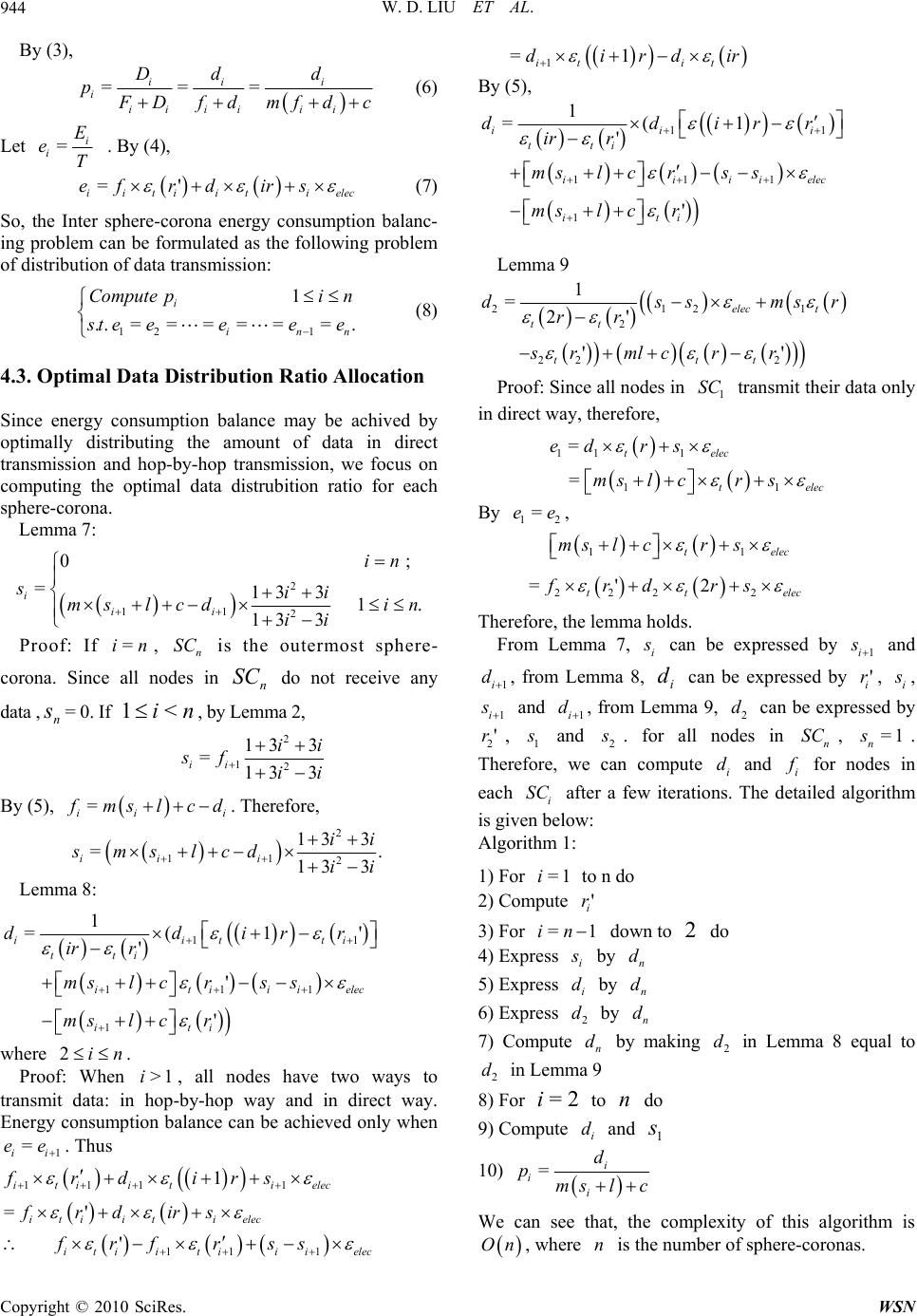

W. D. LIU ET AL. 944
By (3),

===
ii i
ii iiiii
Dd d
p
F
Dfdmfdc 
(6)
Let =i
i
E
eT . By (4),
 
='
iiti itielec
ef rd irs

   (7)
So, the Inter sphere-corona energy consumption balanc-
ing problem can be formulated as the following problem
of distribution of data transmission:
121
1
..= = ====.
i
inn
Computepin
s
te eeee




 (8)
4.3. Optimal Data Distribution Ratio Allocation
Since energy consumption balance may be achived by
optimally distributing the amount of data in direct
transmission and hop-by-hop transmission, we focus on
computing the optimal data distrubition ratio for each
sphere-corona.
Lemma 7:


2
11
2
0 ;
=13 3
1.
13 3
i
ii
in
sii
ms lcdin
ii





 


Proof: If =in, n
SC is the outermost sphere-
corona. Since all nodes in n SC do not receive any
data ,n s= 0. If ni<1 , by Lemma 2,
2
12
13 3
=133
ii ii
sf ii



By (5),

=
ii i
f
mslcd. Therefore,


2
11
2
13 3
=.
13 3
ii i
ii
smslcd ii




Lemma 8:





11
1
=(1'
'
iitti
tti
ddirr
ir r







 
111
'
itiiielec
mslcrss



  

 

1' iti
msl cr 

 

where 2in .
Proof: When >1i, all nodes have two ways to
transmit data: in hop-by-hop way and in direct way.
Energy consumption balance can be achieved only when
1
=
ii
ee
. Thus
 

111 1
1
i tiiti elec
frd irs


 


 
='
i tii ti elec
frdirs

  
 
111
'
itiitiiielec
frf rss


 

 



 
1
=1
it it
dirdir 

By (5),





11
1
=(1
'
iii
tti
ddirr
ir r




 







 
111iii ielec
mslcrs s



   

 

1' iti
msl cr 

 

Lemma 9
 
   
2121
2
1
=2' elec t
tt
dssmsr
rr


 







22 2
''
ttt
srmlc rr  
Proof: Since all nodes in 1 SC transmit their data only
in direct way, therefore,


11 1
=telec edrs

 


11
=telec ms lcrs

   

By 12 =ee,


11telec
ms lcrs

  



222 2
=' 2
t t elec
frd rs

  
Therefore, the lemma holds.
From Lemma 7, i
s
can be expressed by 1i
s

and
1i
d

, from Lemma 8, i d can be expressed by '
i
r, i
s
,
1i
s

and 1i d

, from Lemma 9, 2 d can be expressed by
2'r, 1
s
and 2
s
. for all nodes in n SC , =1
n
s.
Therefore, we can compute i
d and i
f
for nodes in
each i SC after a few iterations. The detailed algorithm
is given below:
Algorithm 1:
1) For =1i to n do
2) Compute '
i
r
3) For =1in

down to 2 do
4) Express i
s
by n d
5) Express i d by n d
6) Express 2 d by n d
7) Compute n d by making 2 d in Lemma 8 equal to
2
d in Lemma 9
8) For 2=i to n do
9) Compute i d and 1 s
10)

=i
ii
d
pmslc


We can see that, the complexity of this algorithm is


On, where n is the number of sphere-coronas.

W. D. LIU ET AL. 945
4.4. Numerical Results and Analysis
We have done numerical analysis , in order to understand
how data compression ratio m influences the data transmission
and reception. The system parameters are set as follows:
= 100R,=10r,=10n,=50/
elec nJ bit

,
= 100/
amp pJ bit

, and =2k.
Figure 9 plots the amount of data received per node
with different sphere-coronas. We can see that, sensors
near the sink node receive more data from hop-by-hop
transmission than those far from the sink node. Especially,
nodes in the outmost sphere-corona (id = 10) receive no
data as no one transmits data to them. This showns our
scheme results in a desirable data distribution to achieve
energy consumption balance. And we can also see that, as
the data compression ratio m sets smaller, the amount of
data received per node in the network becomes also
smaller. This phenomenon manifests that data aggregation
can reduce data transmitted and hence save energy
consumption for WSNs.
Figure 10 plots the ratios of data distribution in
different sphere-coronas. The data distribution ratio
firstly decreases rapidly, then remains constant more or
less in the middle sphere-coronas and finally increases in
the last few sphere-coronas. This can be explained as that,
energy consumption is proportional to the production of
data volume and square of the transmission distance. To
maintain a balanced energy consumption, nodes at the
two ends have a higher distribution ratio because at the
near end nodes have heavy relay burden, but at the far
end it just goes to the opposite: long transmitting
distance but small data volume. And in Figure 10, it is
also easily see that data compression ratio(m) has great
influence on the distribution ratios. When m decreases,
data distribution ratio also decreases at a rate following
lemmas 5-7.
Figure 9. Amount of data received per node for different
sphere-coronas with different data aggregation ratios.
Figure 10. The data distribution ratio different sphere-
coronas with different data aggregation parameters.
5. Network Lifetime Maximization
This section focused on solving the problem of
maximizing network lifetime by achieving energy
consumption balance among all nodes in the network.
For nodes in the outmost sphere-corona n SC ,

 
=*
nntnnt
ef rdnr 

 


=k
nelecampn
mlcdr 

 


k
nelecamp
dR  
When energy consumption balance is achieved, all nodes
have the same energy consumption equalength to n e.
Thus, network lifetime maximization can be formulated
as the following optimization problem:
;
..=, 1,
=.
n
ij
min e
s
teeijn
nr R





5.1. Optimal Number of Sphere Subcoronas
Given n sphere-coronas, i p and i d can be
computed step by step using the algorithm above. By
Theorem 3, the optimal number of sphere subcoronas w*
can be obtained from:

*
=1,2, ,
=in wmaxhi

Where function


=whi is determined by equation
below:


2
22
23
11
421
sin sin
221
ao
ri
LL ww









2
23
11
2=0rww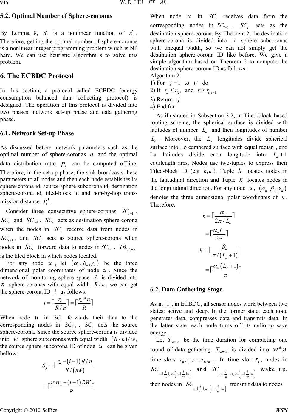





W. D. LIU ET AL. 946
5.2. Optimal Number of Sphere-coronas
By Lemma 8, i
d is a nonlinear function of i r

.
Therefore, getting the optimal number of sphere-coronas
is a nonlinear integer programming problem which is NP
hard. We can use heuristic algorithm s to solve this
problem.
6. The ECBDC Protocol
In this section, a protocol called ECBDC (energy
consumption balanced data collecting protocol) is
designed. The operation of this protocol is divided into
two phases: network set-up phase and data gathering
phase.
6.1. Network Set-up Phase
As discussed before, network parameters such as the
optimal number of sphere-coronas n and the optimal
data distribution ratio i
p can be computed offline.
Therefore, in the set-up phase, the sink broadcasts these
parameters to all nodes and then each node establishes its
sphere-corona id, source sphere subcorona id, destination
sphere-corona id, tiled-block id and hop-by-hop trans-
mission distance '
i
r.
Consider three consecutive sphere-coronas 1i SC

,
i
SC and 1i SC . i SC acts as destination sphere-corona
when the nodes in i SC receive data from nodes in
1i
SC , and i SC acts as source sphere-corona when
nodes in i SC forward data to nodes in1i SC . ,,,ijhk TB
is the tiled block in which nodes located.
For any node u, let


,,
uuu

 be the three
dimensional polar coordinates of node u. Since the
network of monitoring sphere space S is divided into
n sphere-coronas with equal width /Rn, we can get
the sphere-corona ID i as follows:
*
==
/
uu
rrn
iRn R 
When node u in i SC forwards their data to the
corresponding nodes in 1i SC

, i SC acts the source
sphere-corona. Since the source sphere-corona is divided
into w sphere subcoronas with equal width

//Rn w ,
the source sphere subcorona ID of node u can be given
bellow:


1/
=/
u
j
ri Rn
SRnw



1
=u
nwr iRW
R


When node u in i SC receives data from the
corresponding nodes in1i
SC , i SC acts as the
destination sphere-corona. By Theorem 2, the destination
sphere-corona is divided into w sphere subcoronas
with unequal width, so we can not simply get the
destination sphere-corona ID like before. We give a
simple algorithm based on Theorem 2 to compute the
destination sphere-corona ID as follows:
Algorithm 2:
1) For =1j to w do
2) If ,uij rr

and ,1ij rr


3) Return j
4) End for
As illustrated in Subsection 3.2, in Tiled-block based
routing scheme, the spherical surface is divided with
latitudes of number a
L and then longitudes of number
o
L. Moreover, the o L longitudes divide spherical
surface into Lo cambered surface with equal radian , and
La latitudes divide each longitude into 1
a
L

equilength arcs. Nodes use two-tuples to express their
Tiled-block ID (e.g ,hk). Tuple h locates nodes in
the latitudinal direction and Tuple k locates nodes in
the longitudinal direction. For any node u,

,,
uuu


denotes the three dimensional polar coordinates of u,
Therefore,
=2/
u
o
hL




=2
uo
L 




=/1
u
a
kL






1
=ua
L 




6.2. Data Gathering Stage
As in [1], in ECBDC, all sensor nodes work between two
states: active and sleep. In the former state, each node
generates data, compresses data and transmits data. In
the latter state, each node turns off its radio to save
energy.
Let round T be the time duration for completing one
round of data gathering. round T is divided into nw*
time slots 01*1
,, ,
wn



. In time slot i

, nodes in
,
ii
nwiw
ww
SC 
  


and
1,
ii
nwiw
ww
SC 
  


wake up,
then nodes in
,
ii
nwiw
ww
SC 
  


transmit data to nodes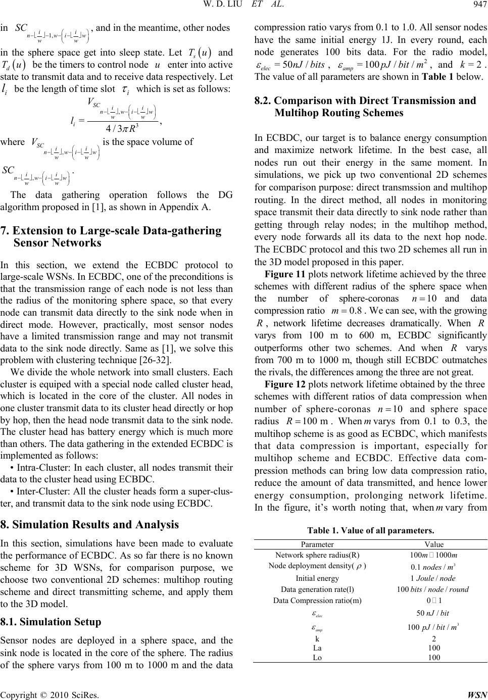

W. D. LIU ET AL. 947
in
1,
ii
nwiw
ww
SC 
  


, and in the meantime, other nodes
in the sphere space get into sleep state. Let


s
Tu and

d
Tu be the timers to control node u enter into active
state to transmit data and to receive data respectively. Let
i
l be the length of time slot i

which is set as follows:
,
3
=,
4/3
SC ii
nwiw
ww
i
V
lR





where
,
SC ii
nwiw
ww
V
 


is the space volume of
,
ii
nwiw
ww
SC 
  


.
The data gathering operation follows the DG
algorithm proposed in [1], as shown in Appendix A.
7. Extension to Large-scale Data-gathering
Sensor Networks
In this section, we extend the ECBDC protocol to
large-scale WSNs. In ECBDC, one of the preconditions is
that the transmission range of each node is not less than
the radius of the monitoring sphere space, so that every
node can transmit data directly to the sink node when in
direct mode. However, practically, most sensor nodes
have a limited transmission range and may not transmit
data to the sink node directly. Same as [1], we solve this
problem with clustering technique [26-32].
We divide the whole network into small clusters. Each
cluster is equiped with a special node called cluster head,
which is located in the core of the cluster. All nodes in
one cluster transmit data to its cluster head directly or hop
by hop, then the head node transmit data to the sink node.
The cluster head has battery energy which is much more
than others. The data gathering in the extended ECBDC is
implemented as follows:
• Intra-Cluster: In each cluster, all nodes transmit their
data to the cluster head using ECBDC.
• Inter-Cluster: All the cluster heads form a super-clus-
ter, and transmit data to the sink node using ECBDC.
8. Simulation Results and Analysis
In this section, simulations have been made to evaluate
the performance of ECBDC. As so far there is no known
scheme for 3D WSNs, for comparison purpose, we
choose two conventional 2D schemes: multihop routing
scheme and direct transmitting scheme, and apply them
to the 3D model.
8.1. Simulation Setup
Sensor nodes are deployed in a sphere space, and the
sink node is located in the core of the sphere. The radius
of the sphere varys from 100 m to 1000 m and the data
compression ratio varys from 0.1 to 1.0. All sensor nodes
have the same initial energy 1J. In every round, each
node generates 100 bits data. For the radio model,
=50/
elec nJ bits

, 2 =100 //
amp pJbit m
 , and =2k.
The value of all parameters are shown in Table 1 below.
8.2. Comparison with Direct Transmission and
Multihop Routing Schemes
In ECBDC, our target is to balance energy consumption
and maximize network lifetime. In the best case, all
nodes run out their energy in the same moment. In
simulations, we pick up two conventional 2D schemes
for comparison purpose: direct transmssion and multihop
routing. In the direct method, all nodes in monitoring
space transmit their data directly to sink node rather than
getting through relay nodes; in the multihop method,
every node forwards all its data to the next hop node.
The ECBDC protocol and this two 2D schemes all run in
the 3D model proposed in this paper.
Figure 11 plots network lifetime achieved by the three
schemes with different radius of the sphere space when
the number of sphere-coronas 10nand data
compression ratio 0.8m

. We can see, with the growing
R, network lifetime decreases dramatically. When R
varys from 100 m to 600 m, ECBDC significantly
outperforms other two schemes. And when R varys
from 700 m to 1000 m, though still ECBDC outmatches
the rivals, the differences among the three are not great.
Figure 12 plots network lifetime obtained by the three
schemes with different ratios of data compression when
number of sphere-coronas 10n and sphere space
radius 100 mR

. Whenmvarys from 0.1 to 0.3, the
multihop scheme is as good as ECBDC, which manifests
that data compression is important, especially for
multihop scheme and ECBDC. Effective data com-
pression methods can bring low data compression ratio,
reduce the amount of data transmitted, and hence lower
energy consumption, prolonging network lifetime.
In the figure, it’s worth noting that, whenmvary from
Table 1. Value of all parameters.
Parameter Value
Network sphere radius(R) 100 1000mm
Node deployment density(

) 0.1 3
/nodesm
Initial energy 1/
J
oulenode
Data generation rate(l) 100 //bitsnoderound
Data Compression ratio(m) 01
elec

50 /nJbit
amp

100 3 //
p
Jbitm
k 2
La 100
Lo 100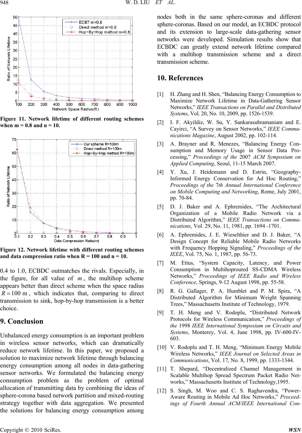

W. D. LIU ET AL. 948
Figure 11. Network lifetime of different routing schemes
when m = 0.8 and n = 10.
Figure 12. Network lifetime with different routing schemes
and data compression ratio when R = 100 and n = 10.
0.4 to 1.0, ECBDC outmatches the rivals. Especially, in
the figure, for all value of m, the multihop scheme
appears better than direct scheme when the space radius
100 mR, which indicates that, comparing to direct
transmission to sink, hop-by-hop transmission is a better
choice.
9. Conclusion
Unbalanced energy consumption is an important problem
in wireless sensor networks, which can dramatically
reduce network lifetime. In this paper, we proposed a
solution to maximize network lifetime through balancing
energy consumption among all nodes in data-gathering
sensor networks. We formulated the balancing energy
consumption problem as the problem of optimal
allocation of transmitting data by combining the ideas of
sphere-corona based network partition and mixed-routing
strategy together with data aggregation. We presented
the solutions for balancing energy consumption among
nodes both in the same sphere-coronas and different
sphere-coronas. Based on our model, an ECBDC protocol
and its extension to large-scale data-gathering sensor
networks were developed. Simulation results show that
ECBDC can greatly extend network lifetime compared
with a multihop transmission scheme and a direct
transmission scheme.
10. References
[1] H. Zhang and H. Shen, “Balancing Energy Consumption to
Maximize Network Lifetime in Data-Gathering Sensor
Networks,” IEEE Transactions on Parallel and Distributed
Systems, Vol. 20, No. 10, 2009, pp. 1526-1539.
[2] I. F. Akyildiz, W. Su, Y. Sankarasubramaniam and E.
Cayirci, “A Survey on Sensor Networks,” IEEE Commu-
nications Magazine, August 2002, pp. 102-114.
[3] A. Brayner and R. Menezes, “Balancing Energy Con-
sumption and Memory Usage in Sensor Data Pro-
cessing,” Proceedings of the 2007 ACM Symposium on
Applied Computing, Seoul, 11-15 March 2007.
[4] Y. Xu, J. Heidemann and D. Estrin, “Geography-
Informed Energy Conservation for Ad Hoc Routing,”
Proceedings of the 7th Annual International Conference
on Mobile Computing and Networking, Rome, July 2001,
pp. 70-84.
[5] D. J. Baker and A. Ephremides, “The Architectural
Organization of a Mobile Radio Network via a
Distributed Algorithm,” IEEE Transactions on Commu-
nications, Vol. 29, No. 11, 1981, pp. 1694 -1701.
[6] A. Ephremides, J. E. Wieselthier and D. J. Baker, “A
Design Concept for Reliable Mobile Radio Networks
with Frequency Hopping Signaling,” Proceedings of the
IEEE, Vol. 75, No. 1, 1987, pp. 56-73.
[7] M. Ettus, “System Capacity, Latency, and Power
Consumption in Multihoprouted SS-CDMA Wireless
Networks,” Proceedings of IEEE Radio and Wireless
Conference, Springs, 9-12 August 1998, pp. 55-58.
[8] R. G. Gallager, P. A. Humblet and P. M. Spira, “A
Distributed Algorithm for Minimum Weight Spanning
Trees,” Massachusetts Institute of Technology, 1979.
[9] T. H. Meng and V. Rodoplu, “Distributed Network
Protocols for Wireless Communication,” Proceedings of
the 1998 IEEE International Symposium on Circuits and
Systems, Monterey, Vol. 4, June 1998, pp. IV-600-IV-
603.
[10] V. Rodoplu and T. H. Meng, “Minimum Energy Mobile
Wireless Networks,” IEEE Journal on Selected Areas in
Communications, Vol. 17, No. 8, 1999, pp. 1333-1344.
[11] T. Shepard, “Decentralized Channel Management in
Scalable Multihop Spread Spectrum Packet Radio Net-
works,” Massachusetts Institute of Technology,1995.
[12] S. Singh, M. Woo and C. S. Raghavendra, “Power-
Aware Routing in Mobile Ad Hoc Networks,” Proceed-
ings of Fourth Annual ACM/IEEE International Con-

W. D. LIU ET AL. 949
ference on Mobile Computing and Networking, Dallas,
October 1998, pp. 181-190.
[13] I. Akyildiz, W. Su, Y. Sankarasubramaniam and E. Cyirci,
“Wireless Sensor Networks: A Survey,” Computer Net-
works, Vol. 38, No. 4, 2002, pp. 393-422.
[14] F. Zhao and L. Guibas, “Wireless Sensor Networks: An
Information Processing Approach,” Morgan Kaufmann
Publishers, Massachusetts, 2004.
[15] C. Efthymiou, S. Nikoletseas and J. Rolim, “Energy
Balanced Data Propagation in Wireless Sensor Net-
works,” Wireless Networks, Vol. 12, No. 6, 2006, pp.
691-707.
[16] W. Guo, Z. Liu and G. Wu, “An Energy-Balanced
Transmission Scheme for Sensor Networks,” Proceed-
ings of the First International Conference Embedded
Networked Sensor Systems, Los Angeles, 5-7 November
2003, pp. 300-301.
[17] O. Powell, P. Leone and J. Rolim, “Energy Optimal Data
Propagation in Wireless Sensor Networks,” Journal of
Parallel and Distributed Computing, Vol. 67, No. 3, 2007,
pp. 302-317.
[18] H. Zhang, H. Shen and Y. Tan, “Optimal Energy
Balanced Data Gathering in Wireless Sensor Networks,”
Proceedings of the 21st International Parallel and
Distributed Processing Symposium, Long Beach, 26-30
March 2007, pp. 1-10.
[19] A. Zhao, J. Yu and Z. Li, “A Data Aggregation Scheme
in Wireless Sensor Networks for Structure Monitoring,”
Proceedings of the 2009 International Conference on
Information Management, Innovation Management and
Industrial Engineering, Xi’an, 26-27 December 2009,
Vol. 4, pp. 623-626.
[20] J. N. Al-Karaki, R. Ul-Mustafa and A. E. Kamal, “Data
Aggregation and Routing in Wireless Sensor Networks:
Optimal and Heuristic Algorithms,” Computer Networks,
Vol. 53, No. 7, 2009, pp. 945-960.
[21] W. M. Lee and V. W. Wong, “E-Span and LPT for Data
Aggregation in Wireless Sensor Networks,” Computer
Communications, Vol. 29, No. 13-14, 2006, pp. 2506-
2520.
[22] W. Liao, Y. Kao and C. Fan, “Data Aggregation in
Wireless Sensor Networks Using Ant Colony Algori-
thm,” Journal of Network and Computer Applications,
Vol. 31, No. 4, 2008, pp. 387-401.
[23] S. Ozdemir and Y. Xiao, “Secure Data Aggregation in
Wireless Sensor Networks: A Comprehensive Over-
view,” Computer Networks, Vol. 53, No. 12, 2009, pp.
2022-2037.
[24] S. Ozdemir, “Functional Reputation Based Reliable Data
Aggregation and Transmission for Wireless Sensor Net-
works,” Computer Communications, Vol. 31, No. 17
2008, pp. 3941-3953.
[25] W. R. Heinzelman, A. Chandrakasan and H. Balakrishnan,
“Energy-Efficient Communication Protocol for Wireless
Microsensor Networks,” Proceedings 33rd Hawaii Inter-
national Conference System Sciences, Vol. 8, 2000, p.
8020.
[26] A. S. Malik, J. Kuang, J. Liu and W. Chong, “Energy
Consumption and Lifetime Analysis in Cluster-Based
Wireless Sensor Networks for Periodic Monitoring
Applications,” Proceedings of the 2009 International
Conference on Networks Security, Wireless Communica-
tions and Trusted Computing, Wuhan, Vol. 1, 25-26
April 2009, pp. 657-661.
[27] Z. Zhang, “Towards Cluster Based Wireless Sensor
Network Deployment Management and Network
Coverage Verification,” Proceedings of the 11th Asia-
Pacific Symposium on Network Operations and Manage-
ment: Challenges For Next Generation Network Opera-
tions and Service Management, Beijing, Vol. 5297, 22-24
October 2008, pp. 197-206.
[28] Y. Huang, N. Wang and M. Chen, “Performance of a
Hierarchical Cluster-Based Wireless Sensor Network,”
Proceedings of the 2008 IEEE international Conference
on Sensor Networks, Ubiquitous, and Trustworthy
Computing, Taichung, 11-13 June 2008, pp. 349-354.
[29] H. Su and X. Zhang, “Optimal Transmission Range for
Cluster-Based Wireless Sensor Networks with Mixed
Communication Modes,” Proceedings of the 2006 inter-
national Symposium on World of Wireless, Mobile and
Multimedia Networks, Buffalo, 26-29 June 2006, pp.
244-250.
[30] Y. Huang, N. Wang, C. Chen, J. Chen and Z. Guo,
“Equalization of Energy Consumption at Cluster Head for
Prolonging Lifetime in Cluster-Based Wireless Sensor
Networks,” WSEAS Transactions on Communications,
Vol. 8, No. 5, May 2009, pp. 427-436.
[31] A. T. Hoang and M. Motani, “Collaborative Broadcasting
and Compression in Cluster-Based Wireless Sensor
Networks,” ACM Transactions on Sensor Networks, Vol.
3, No. 3, 2007, p. 17.
[32] Y. Chang, J. Huang and T. Juang, “Dependable Data
Aggregation on Cluster-Based Wireless Sensor Net-
works,” Proceedings of the 11th Conference on 11th
WSEAS international Conference on Communications,
Crete Island, Vol. 11, 26-28 July 2007, pp. 300-305.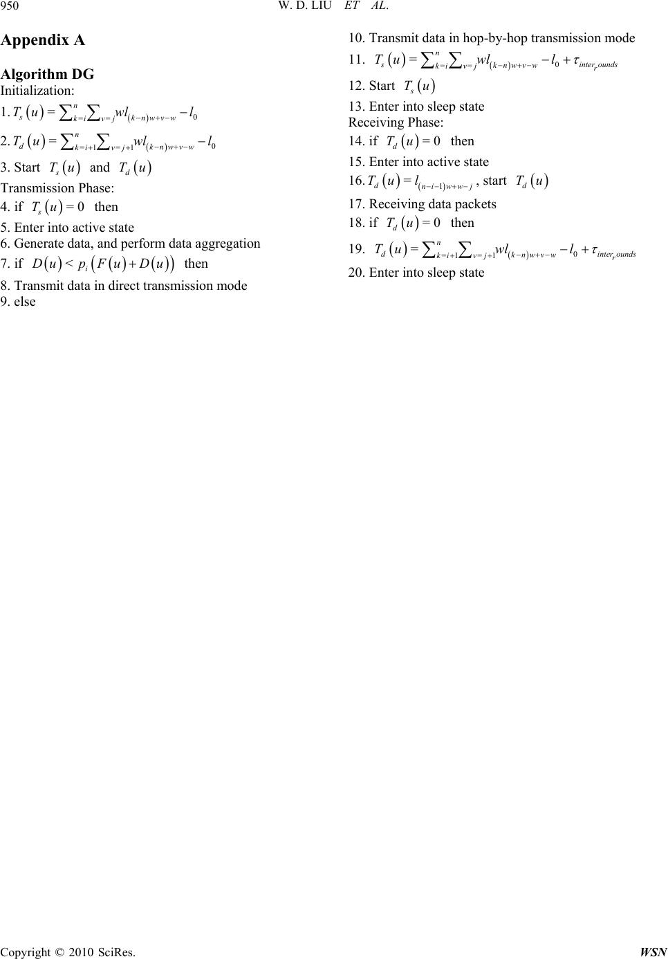

W. D. LIU ET AL. 950
Appendix A
Algorithm DG
Initialization:
1.


0
==
=n
sknwvw
ki vj
Tuwll



2.


0
=1= 1
=n
dknwvw
ki vj
Tuwl l

 

3. Start

s
Tu and

d
Tu
Transmission Phase:
4. if

=0
s
Tu then
5. Enter into active state
6. Generate data, and perform data aggregation
7. if
  
<i DupFuDu then
8. Transmit data in direct transmission mode
9. else
10. Transmit data in hop-by-hop transmission mode
11.


0
==
=n
s
inter ounds knwvw
ki vjr
Tuwll 



12. Start


s
Tu
13. Enter into sleep state
Receiving Phase:
14. if


=0
d
Tu then
15. Enter into active state
16.



1
=
dniww j
Tu l


, start

d
Tu
17. Receiving data packets
18. if


=0
d
Tu then
19.


0
=1= 1
=n
dinter ounds
knwvw
ki vjr
Tuwl l 

 

20. Enter into sleep state