Wireless Sensor Network, 2010, 2, 924-935
doi:10.4236/wsn.2010.212111 Published Online December 2010 (http://www.scirp.org/journal/wsn)
Integer Programming Formulations for Maximum
Lifetime Broadcasting Problems
in Wireless Sensor Networks
Roberto Montemanni
Istituto Dalle Molle di Studi sull’Intelligenza Artificiale,
Lugano, Switzerland
Received November 2, 2010; revised November 10, 2010; accepted November 17, 2010
Abstract
Approaches based on integer linear programming have been recently proposed for topology optimization in
wireless sensor networks. They are, however, based on over-theoretical, unrealistic models. Our aim is to
show that it is possible to accommodate realistic models for energy consumption and communication proto-
cols into integer linear programming. We analyze the maximum lifetime broadcasting topology problem and
we present realistic models that are also shown to provide efficient and practical solving tools. We present a
strategy to substantially speed up the convergence of the solving process of our algorithm. This strategy in-
troduces a practical drawback, however, in the characteristics of the optimal solutions retrieved. A method to
overcome this drawback is discussed. Computational experiments are reported.
Keywords: Sensor Networks, Mixed Integer Linear Programming, Energy Models, Topology Optimization
1. Introduction
Since the very beginning of research in the area of wire-
less sensor networks, one of the major issues has been
saving power. This optimization is typically faced during
the design, and prior the deployment of the nodes of a
network. Such a high attention for this factor is easy to
identify: the nodes of the network (devices) are typically
equipped with low capacity, tiny batteries, and they have
to stay alive in the longest possible time horizon. This in
an environment usually characterized by reduced acces-
sibility. A tight management of the power budget is im-
posed by all these factors. Another peculiarity of sensor
networks is that the largest share of power consumption
is normally due to communication rather than to compu-
tation, sensing and state-changing activities [1,2]. We
will base our study on this assumption.
Wireless sensor networks are typically used in com-
manding actuators, monitoring events or measuring val-
ues at locations where people cannot reach easily, or
where a long term sensing task is required. Examples of
applications are habitat monitoring [3], civil structural
monitoring [4] and environmental monitoring [5]. Nodes
can usually be characterized as low cost devices, and are
to be deployed in a potentially inaccessible area. Re-
charging the sensors after the deployment might there-
fore not be an option, both for logistic and economical
reasons. In this context, energy-efficiency becomes per-
haps the most important design criteria for sensor net-
works, since it directly impacts on the time the network
itself is kept in operation. Many sensor network applica-
tions are intrinsically about dissemination of information
from a well-identified source node. It is therefore critical
to identify energy efficient network topologies, opti-
mized according to the type of communications that has
to be supported. In this paper we will concentrate on
broadcasting topologies, where a piece of information
has to be sent from a source node to all of the other
nodes of the network. We will assume to work on a static
network, i.e. nodes do not move after the deployment.
Researchers have proposed many different mechan-
isms for achieving energy-efficiency in sensor networks.
For example, transmission power control in radios, peri-
odic cycling of nodes’ activity schedules [6], in-network
processing of sensor data [7] and aggregation [8] for da-
ta-gathering applications. In most of the communication
models adopted in these studies, the total energy cost for
a transmitted bit is computed as the cost of a transmis-
sion over a wireless channel over a certain distance. In
some cases, the cost due to reception by the destination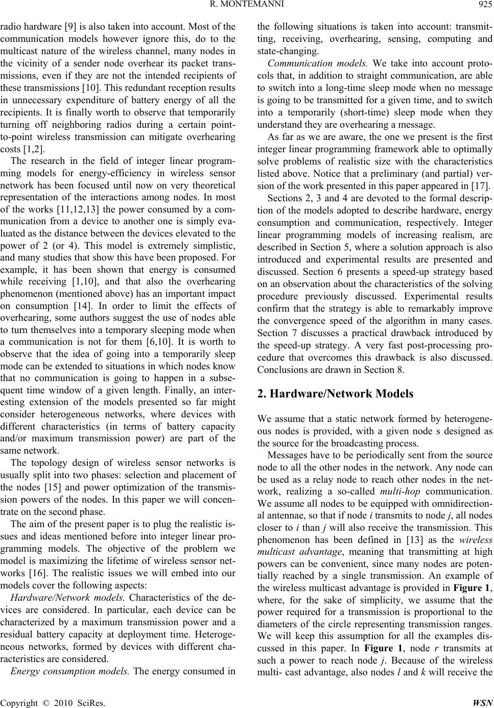

R. MONTEMANNI 925
radio hardware [9] is also taken into account. Most of the
communication models however ignore this, do to the
multicast nature of the wireless channel, many nodes in
the vicinity of a sender node overhear its packet trans-
missions, even if they are not the intended recipients of
these transmissions [10]. This redundant reception results
in unnecessary expenditure of battery energy of all the
recipients. It is finally worth to observe that temporarily
turning off neighboring radios during a certain point-
to-point wireless transmission can mitigate overhearing
costs [1,2].
The research in the field of integer linear program-
ming models for energy-efficiency in wireless sensor
network has been focused until now on very theoretical
representation of the interactions among nodes. In most
of the works [11,12,13] the power consumed by a com-
munication from a device to another one is simply eva-
luated as the distance between the devices elevated to the
power of 2 (or 4). This model is extremely simplistic,
and many studies that show this have been proposed. For
example, it has been shown that energy is consumed
while receiving [1,10], and that also the overhearing
phenomenon (mentioned above) has an important impact
on consumption [14]. In order to limit the effects of
overhearing, some authors suggest the use of nodes able
to turn themselves into a temporary sleeping mode when
a communication is not for them [6,10]. It is worth to
observe that the idea of going into a temporarily sleep
mode can be extended to situations in which nodes know
that no communication is going to happen in a subse-
quent time window of a given length. Finally, an inter-
esting extension of the models presented so far might
consider heterogeneous networks, where devices with
different characteristics (in terms of battery capacity
and/or maximum transmission power) are part of the
same network.
The topology design of wireless sensor networks is
usually split into two phases: selection and placement of
the nodes [15] and power optimization of the transmis-
sion powers of the nodes. In this paper we will concen-
trate on the second phase.
The aim of the present paper is to plug the realistic is-
sues and ideas mentioned before into integer linear pro-
gramming models. The objective of the problem we
model is maximizing the lifetime of wireless sensor net-
works [16]. The realistic issues we will embed into our
models cover the following aspects:
Hardware/Network models. Characteristics of the de-
vices are considered. In particular, each device can be
characterized by a maximum transmission power and a
residual battery capacity at deployment time. Heteroge-
neous networks, formed by devices with different cha-
racteristics are considered.
Energy consumption models. The energy consumed in
the following situations is taken into account: transmit-
ting, receiving, overhearing, sensing, computing and
state-changing.
Communication models. We take into account proto-
cols that, in addition to straight communication, are able
to switch into a long-time sleep mode when no message
is going to be transmitted for a given time, and to switch
into a temporarily (short-time) sleep mode when they
understand they are overhearing a message.
As far as we are aware, the one we present is the first
integer linear programming framework able to optimally
solve problems of realistic size with the characteristics
listed above. Notice that a preliminary (and partial) ver-
sion of the work presented in this paper appeared in [17].
Sections 2, 3 and 4 are devoted to the formal descrip-
tion of the models adopted to describe hardware, energy
consumption and communication, respectively. Integer
linear programming models of increasing realism, are
described in Section 5, where a solution approach is also
introduced and experimental results are presented and
discussed. Section 6 presents a speed-up strategy based
on an observation about the characteristics of the solving
procedure previously discussed. Experimental results
confirm that the strategy is able to remarkably improve
the convergence speed of the algorithm in many cases.
Section 7 discusses a practical drawback introduced by
the speed-up strategy. A very fast post-processing pro-
cedure that overcomes this drawback is also discussed.
Conclusions are drawn in Section 8.
2. Hardware/Network Models
We assume that a static network formed by heterogene-
ous nodes is provided, with a given node s designed as
the source for the broadcasting process.
Messages have to be periodically sent from the source
node to all the other nodes in the network. Any node can
be used as a relay node to reach other nodes in the net-
work, realizing a so-called multi-hop communication.
We assume all nodes to be equipped with omnidirection-
al antennae, so that if node i transmits to node j, all nodes
closer to i than j will also receive the transmission. This
phenomenon has been defined in [13] as the wireless
multicast advantage, meaning that transmitting at high
powers can be convenient, since many nodes are poten-
tially reached by a single transmission. An example of
the wireless multicast advantage is provided in Figure 1,
where, for the sake of simplicity, we assume that the
power required for a transmission is proportional to the
diameters of the circle representing transmission ranges.
We will keep this assumption for all the examples dis-
cussed in this paper. In Figure 1, node r transmits at
such a power to reach node j. Because of the wireless
multi- cast advantage, also nodes l and k will receive the

R. MONTEMANNI 926
message, since they are closer to r than j.
We assume the power necessary to transmit from each
node of the network to each other node to be known in
advance. It usually depends on the characteristics of the
terrain in which nodes are deployed. We will refer to the
power necessary to transmit a bit of information from
node i to node j as pij. We also assume to know, for each
node i, its maximum transmission power MPi and its
residual battery capacity at deployment time, referred to
as capi. To represent the problem in mathematical terms,
we can therefore define a complete directed graph G =

,VA, where V is the set of nodes of the network, and
A is a set of arcs corresponding to all the possible
one-hop communications between the nodes of the net-
work: 
,ij
∈ A ∀ i, j ∈ V. Power pij can be then seen as
a label associated with arc

,ij.
It is important to stress that the models and methods
we will discuss in Section 5 are independent on the mod-
el used to estimate power requirements.
Notice that placement and characteristics of the nodes
are regarded as the output of a previous optimization
phase.
3. Energy Consumption Models
In most of the power-optimization studies proposed so
far [2,11,13,16], very simplistic, basic energy models
were considered: typically anything different from
transmitting power pij (see Section 2) was classified as
negligible, and therefore ignored. On the other hand,
many works exist to precisely quantify the energy con-
sumption involved in the different operations carried out
by the nodes [10].
In wireless sensor networks nodes consume energy
while sensing, changing state, computing and communi-
cating. Sensing, state-changing and computing activities
are strictly application dependent, and we therefore as-
sume to have an estimate for the energy consumption
involved in them. Different is the situation for the power
consumed in communication activities. We assume that
energy is consumed when a packet is sent, received, and
overheard, i.e. when a node receives a message that was
not destined to it. The model we adopt is that proposed in
[14]. In the network of Figure 1, node k (which has al-
ready received the transmission from r) overhears the
communication from node j to node m, being closer to j
than m. Considering the overhearing phenomenon makes
the energy model particularly realistic.
Let us formally define what we will refer to as the ad-
vanced energy model. Energy consumption in one bit
data transmission, tx

, is proportional to the transmitting
power p of the transmitting node:
p
tx txelec
 
(1)
where txelec

is the energy consumption by transmitter
electronics,

is an amplifier characteristic constant
(that depends on the media) .
Energy consumption in reception is independent of the
transmitting power, and refers to the energy consumed
by receiver electronics. We will refer to the energy dis-
sipated for receiving a bit of information as rc

.
The logic for the calculation of the energy dissipated
in overhearing activities oh

) is the same as for the cal-
culation of the energy required while receiving. In this
paper, following the approach already adopted in [14],
we will assume that the energy consumed while over-
hearing is exactly the same as the energy consumed
when receiving: oh

= rc

. This assumption leads to a
simplified notation (without oh

), which is adopted in
the reminder of the paper.
The energy dissipated in computing, state-changing
and sensing has finally to be considered. As previously
observed, this quantity is extremely application-
dependent, and has to be estimated case by case. We
therefore assume to know in advance the cumulative
energy dissipated by each node i in these tasks during
each broadcasting cycle. We will refer to it as

s
ci

.
Notice that this quantity is not necessarily the same for
all the nodes, and that the energy dissipated between two
consecutive broadcasting cycles is also counted here: if
the devices are able to switch themselves into a tempo-
rary sleeping mode between two consecutive broadcast-
ing cycles, the energy consumed will be low, otherwise
the energy dissipated while in idle state will be higher.
4. Communication Models
Two different communication models are considered in
this paper, based on two different communication proto-
cols implemented in the reality.
The standard communication protocol considered is
that working on devices without the capability of
switching into a temporary sleep mode when they under
Figure 1. The wireless multicast advantage [13]. Example of
overhearing phenomenon.

R. MONTEMANNI 927
stand that a message that is being transmitted is not of
their interest. The smart communication protocol is that
associated with advanced devices able to switch into a
temporary sleep state. Notice that this protocol implies
the presence of header messages, used to identify the
subsequent data messages. Header messages will intui-
tively contain the information of the data message that
will follow, together with the length of the message itself.
Consider again the example in Figure 1. If the smart
protocol is in use, node k can temporarily turn itself off
when it understands that the transmission generated from
node j is not of its interest (it is about a message already
received at k while transmitted from r).
It is easy to foresee that a smart communication pro-
tocol can be very useful for mitigating power consump-
tion due to overhearing at the nodes. This justifies the
increase in the complexity of both the hardware of the
devices and the communication protocol.
In the reminder of the paper we will refer to the di-
mension of the data packet that has to be broadcasted
from the source node to all the other nodes of the net-
work as
D
. We will also indicate with the Hdimension
of the header of the data packet, which will contain a
message-id and the dimension of the following data
packet. The header will be sent immediately before the
data packet and (if a smart communication protocol is
used) nodes hearing it will know if they have received
the message already, and undertake the appropriate ac-
tions.
5. Integer Linear Programming
Formulations
5.1. Maximum Transmission Powers
According to Section 2, a maximum transmission power
i
M
P is given for each node . This parameter is, in fact,
transparent to the integer linear programming models we
will propose.
Consider the case where the transmission power re-
quired to transmit from a node i to another node j (pij) is
greater than i
M
P. It means that node i is not able to
transmit to j in a single hop. We can therefore modify pij
and assign an infinite value to it. This will rule out the
single-hop communication i−j from every feasible solu-
tion of our models. Formally, we will modify the power
requirements for the one hop communication for some
pairs of nodes

,ij, as follows:
:
iji ij
pMP p
(2)
5.2. Skeleton Structure
The integer linear programming models we propose are
all based on the common idea of skeleton structure. Such
an approach is common in the literature of topology op-
timization (see, for example [11,18]). Each feasible solu-
tion is characterized by at least a skeleton, which ensures
that all the nodes of the network receive, in a multi-hop
fashion, the message broadcasted from the source node s.
For example, in Figure 1 a skeleton of the broadcasting
structure is the depicted directed tree (arborescence)
rooted in s. Notice that all the transmission powers of the
nodes are such that the arcs of the arborescence are cov-
ered. The vice-versa is not true: not all the arcs covered
by the power assignment are part of the arborescence. In
our approach, we will adopt a structure that contains (is a
superset of) an arborescence.
We define the skeleton in terms of mixed integer pro-
gramming formulation. The transmission power


ri
assigned to a generic node i will assume either a value of
zero or of pij, for some
j
V

. A set of variables x is
then introduced to describe the transmission power of
each node. For each pair of nodes i,j ∈ V we have:


1 if r
0 otherwiise
ij
ij
ip
x




 (3)
It is easy to verify that if xij = 1, then all the nodes
closer to i than j will also receive (or overhear) the
transmission from i. We have the following definition:
Definition 1 Given two nodes i and j such that pij < +∞,
we define N as follows:
 

:
i
NjkV pikpij (4)
The set


i
Nj contains the nodes of V which are not
closer to i than j. Notice that j ∈

i
Nj
. The set Skl of
all possible skeleton structures defined on graph G, is
described by the following constraints:

\
,
1 CV,sC
kVC
ij
iC
jU Nik
x



 
 (5)
1
ij
jV
x
iV


 (6)
0
is
iV
x


 (7)




0,1 ,
ij
xij

 (8)
In constraints (5), C is used to model each non-empty
subset of V containing the source node s. For each one of
these sets, there is a constraint in the model specifying
that at least one of the nodes of C must transmit at such a
power to reach at least one node out of C. Constraints (6)
state that at most one arc among the outgoing ones from
each node must be active. Constraint (7) states that none
of the incoming arcs of the source node can be active.
Constraints (8) define variables domain.

R. MONTEMANNI 928
5.3. Objective Function
In our optimization we seek for a broadcasting structure
that maximizes the number of broadcasting cycles sup-
ported before the first device runs out of battery. The
power consumption at each node of the network and its
initial battery capacity are taken into account. This
translates into counting the number of broadcasting
cycles supported by each node, and choosing the smallest
value.
Given an skeleton x ∈ Skl, we will refer to the power
consumed in a single broadcasting cycle by node i
as 
,pci x. The problem studied in the paper can be
formally defined through the following equation:

max min,
i
iV xSkl
cap
npci x








(9)
where n is the number of broadcasting cycles supported
by the optimal broadcasting structure. Constraints (9)
cannot be directly expressed in terms of mixed integer
linear programming, because the variables of the model
are at the denominator. It is however possible to mani-
pulate (9) in order to obtain an equivalent description
that can be expressed as a mathematical program. If we
invert the fraction in (9), we end up with an expression
for the inverse of the number of cycles supported by each
node. The min and max operators have also to be com-
plemented as a consequence of the inversion. We obtain
the following equation:

,
1min max
xSkl iV i
pci x
ncap










(10)
from which it is trivial to obtain the original value of n,
once (10) has been solved. Starting from (10), and as-
suming that we are able to find a linear expression for

,pci x, a mixed integer linear program is easy to ob-
tain. First we have to get rid of the nested max operator.
This can be done by introducing a free variable z, and by
transforming (10) into the following system, which is
linear if we can find a linear expression for

,pcix:
1min z
n (11)

,
.. z
i
pci x
s
tiV
cap
 (12)
x
Skl (13)
z
IR (14)
Notice that constraints (13) can be substituted by their
linear expression, which is provided by inequalities (5),
(6) and (7).
What remains to be disclosed is the expression in li-
near terms of

,pci x. In Subsections 5.4, 5.5 and 5.6 we
will see how this can be done for different combinations
of the energy and communication models described in
Sections 3 and 4.
5.4. Model M1: Basic Energy Model, Basic
Communication Protocol
The energy and communication models adopted for this
formulation are those commonly used in the theoretical
studies for minimum power broadcasting structures
[11,13] and maximum lifetime broadcasting structures
[16]. A very high level of abstraction is implied, and
therefore these models are often regarded as too theoreti-
cal.
The energy model does not take into account the
energy consumed while receiving and overhearing (rc

= oh

= 0), flattering down also the role of the commu-
nication protocol (a smart protocol is not of any help if
overhearing is not taken into account).
It is important to notice that this model, although not
of particular practical interest, has been considered in
this study because it provides a sort of a bridge between
the very theoretical mathematical programming models
provided so far [11,13,18], and the more realistic models
M2 and M3 we will describe in Sections 5.5 and 5.6.
The model is composed of constraints (11), (5), (6), (7)
and (14), plus the following inequalities (15), that make
constraints (12) explicit.

 




\
z
tr ij
sc
ij
jV i
ii
HD p
i
x
iV
cap cap




 
 (15)
The first term in the right hand side of constraints (15)
models the fraction of the available energy consumed by
nodes during each broadcasting cycle for sensing, com-
puting and state-changing. The second term models the
fraction of battery consumed for transmitting during each
cycle. Notice that for each node i, at most one of the xijs
will take value 1 in each feasible solution, because of
constraints (5), (6) and (7). Consequently, in each one of
constraints (15), no more than one x variable will take
value 1.
5.4. Model M2: Advanced Energy Model, Basic
Communication Protocol
Model M2 is for problems described through the ad-
vanced communication models presented in Section 3,
but where no smart communication protocol is imple-
mented (see Section 4).
Beside constraints (11), (5), (6), (7) and (14), model
M2 includes the following inequalities (16), that make
constraints (12) explicit.

R. MONTEMANNI 929

 




 


\
\
z
j
tr ij
sc
ij
jV i
ii
rc
jk
jV ii
kN i
HDp
i
x
cap cap
HD xiV
cap












(16)
The first term in the right-hand-side of constraints (16)
has the same meaning as in constraints (15). The first
sum represents the fraction of the available energy dissi-
pated by node i for data transmission. Notice that if xij= 0
∀ j ∈ V, it means that node i does not transmit in the
current skeleton, and consequently this term will give a
contribution of 0. The second sum represents the fraction
of the available energy dissipated while receiving and
overhearing. Notice that this contribution is paid for each
communication reaching node i.
5.6. Model M3: Advanced Energy Model, Smart
Communication Protocol
The integer linear programming model presented in this
section builds up on that proposed in Subsection 5.5. The
difference is that now the advantages derived from the
use of a smart communication protocol (which is useful
when nodes can go in a sleep mode when they are not
interested in a transmission) have been taken into ac-
count.
This model can be regarded as the most realistic model
we present in this paper, and is based on the following
constrains: (11), (5), (6), (7), (14), plus (17) and (18):

 




 

 

\
\
z
+ \8
j
tr ij
sc
ij
jV i
ii
rc
rc
jk
jV iii
kN i
HD p
ix
cap cap
HD
HxiV
cap cap













(17)








\
\
z
j
tr sj
sc
ij
jV s
si
rc
jk
jV ss
kN s
HDp
s
x
cap cap
Hx
cap











(18)
The first term in the right-hand-side of inequalities (17)
and (18) is the usual fractional power consumption due
to sensing, computing and state-changing during each
broadcasting cycle. The first sum of constraints (17) is
the same as in constraint (16). The second sum models
overhearing at node i, following the same reasoning al-
ready seen for the second sum of (16): the sum contains
all the communications potentially overheard by i, that
will give a contribution or not to the sum according to
the value of the x variables associated. The last term fi-
nally models the fractional energy consumption due to
data reception (not overhearing). This contribution is
based on the consideration that each node (apart from the
source s) will receive the data packet exactly once. No-
tice that each node will be able to classify a packet as
already received by analyzing the corresponding header.
The only difference between constraints (17) and (18), is
that in the right-hand-side of the former, the last term of
(17) is not present, since the root will not receive any
message, being the node from which the broadcasting is
actually originated.
5.7. Solution Method
The bottleneck of the three mixed integer linear pro-
gramming formulations described in Subsections 5.4, 5.5
and 5.6 is represented by the common constraints (5).
Specifically, constraints (5) are present in huge number
(exponential in the number of devices in the network),
and create difficulties to the solvers used to handle the
models. To overcome these problems, we adopted a
strategy commonly used in similar cases (see, for exam-
ple, [19]), and that can be summarized as follows. It is an
iterative approach, which in the beginning does not con-
sider any of the constraints (5), and adds them only when
violated by the current (infeasible) solution.
In the reminder of this section we will refer to a ge-
neric mixed integer linear program IP. Formulations M1,
M2 and M3 (initially without constraints (5)) can all
substitute the generic formulation IP.
At each iteration, the integer linear program IP is
solved to optimality and the values of the x variables in
the optimal solution are examined. If the arcs corres-
ponding to variables with value 1 (we will refer to them
as active variables) form a directed structure that reaches
all the devices of the network (skeleton), then the prob-
lem has been solved to optimality, and we can stop. Oth-
erwise, a set of violated constraint of type (5) is identi-
fied (by solving maximum flow problem, see [20]) and
added to the mixed integer linear program IP, and the
process is repeated. In case the optimal solution has not
been found, let us consider the arcs corresponding to the
active x variables of the last available solution. We de-
fine the set C of the constraint (5) as the set of nodes that
can be reached from the source s using arcs associated
with active x variables only. The new constraint added
makes the current solution infeasible for the newly aug-
mented problem IP, forcing the solver to move to a dif-
ferent solution in the next iteration. Iteration after itera-
tion, the incumbent solution x should get closer and
closer to feasibility with respect to the original problem,
being it of type M1, M2 or M3. The algorithm is summa-
rized in Figure 2, where a pseudo-code is presented.
A well-known technique (see, for example, [20]) to

R. MONTEMANNI 930
Figure 2. A pseudo-code for the algorithm used to solve
integer linear formulations M1, M2 and M3.
speed up the algorithm described above first considers
LR, the linear relaxation of the mixed integer linear pro-
gramming formulation IP. It is obtained by substituting
constraints (8) with the following one:


01 ,
ij
xij  (19)
The algorithm described in Figure 2 is run on LR. When
there are no more violated cuts, which means LR has
been solved to optimality, the original problem IP is con-
sidered, and the algorithm presented in Figure 2 is run
again, starting from the set of cuts identified for the li-
near relaxation LR (instead of an empty set). The aim of
such a technique is to reduce the number of mixed integ-
er programs that have to be solved to identify violated
cuts, in the hope that many of the cuts were already iden-
tified on the linear relaxation LR, which is off course
much easier to solve, not having binary variables. We
will adopt this strategy in our implementation.
5.8. Experimental Results
Computational experiments have been carried out on
random networks with up to 80 nodes. The signal propa-
gation model adopted for the experiments is the one
commonly used in the literature (see, for example, [13,
21]). For a node i of the network, the power required to
reach another node j is given by:

2
ij ij
pd (20)
The data and energy parameter settings adopted for the
simulations are the following ones:
D
= 500 bites,H=
10 bites, = 0.1 nJ/bit/m2, txelec

= 50 nJ/bit, rc

=oh

= 50 nJ/bit, 
rc i

= 50 nJ/cycle. For every problem
considered, the capacity capi associated with the battery
of node i (expressed in Joule for the sake of simplicity) is
chosen at random from the interval [1000; 5000].
Problems with |V| (number of nodes) ∈ {20, 30, 40,
50, 60, 70, 80} have been considered. Ten instances have
been generated at random on a 100×100 grid for each
value of |V|. Tests have been carried out on a computer
equipped with an Intel Pentium M 1.73GHz processor
and 512 MB of memory. IBM ILOG CPLEX 12.1
(http://www.cplex.com) has been used to solve mixed
integer linear programs. A maximum computation time
of 3 hours has been allowed for each combination (model,
instance).
Results are summarized in Table 1, where for each
combination (model, |V|) we report average and standard
deviation for the number of cuts (5) added (both on the
linear relaxation phase and in total), and for the compu-
tational time in seconds. Statistics are computed on the
instances solved to optimality (reported in the second
column of the table) over the ten considered for each line
of the table.
The computational results suggest that two of the three
methods we developed are able to handle networks with
up to 80 nodes in 3 hours. This result is encouraging be-
cause it proves that the approach we propose is suitable
to be used on networks with sizes of practical interests. A
deeper analysis of Table 1 suggests that model M1 re-
quires much more iterations (cuts (5)) than M2 and M3
to converge to the optimal solution. Analogous consider-
ations can be done for the computation times required to
solve the different models. Another important indication
emerging from Table 1 is about the performance degra-
dation as the number of nodes increases. Models M2 and
M3 clearly scale up much better than M1.
The most important outcome of Table 1 is however
probably the indication that handling more complex
models (M2 and M3) leads to easier problems (from a
computational point of view) than the simpler models
considers so far in the literature (M1). Basically, M2 and
M3 provide better models both from a theoretical (level
of realism) and practical (solution times) point of view.
It is finally important to observe that the standard
deviation of all the indicators reported in Table 1 is high.
This indicate that the performance of the exact methods
we propose tend to be instance-dependent.
6. A Speed-up Strategy
Classic valid inequalities for integer linear models of
broadcasting problems on wireless networks can be eas-
ily adapted to our problem (we refer the interested reader
to [8,20,21]). However, we discovered that a strategy
different from (and usually not compatible with) classic
valid inequalities is more effective and efficient for the
maximum lifetime problems on wireless networks, in a
framework like the one we propose.
Notice that in the reminder of the paper we will concen-
trate, for short, on formulation M2, but all the results can
be trivially adapted to both the other models M1 and M3.
The idea exploits a characteristic of the problem: the
objective function cost is only determined by the node i
with the shortest lifetime of the current topology. In this
context, it is easy to observe that if all the other nodes of
the network transmit at the maximum possible power
such that their lifetime is not shorter than that of node i,

R. MONTEMANNI 931
Table 1. Computational results.
V Solved LR cuts (5) addedTotal cuts(5) addedSeconds
(over 10) avg stdev avg stdev avg stdev
Model M1
20 10 69.90 16.78 73.60 17.27 0.30 0.28
30 10 146.40 41043 153.20 36.71 12.79 23.54
40 4 247.50 49.84 278.25 53.56 485.23658.91
50 3 288.67 27.97 363.33 90.29 1441.73913.65
60 1 415.00 0.00 415.00 0.00 558.000.00
70 0 - - - - - -
80 0 - - - - - -
Model M2
20 10 68.90 16.13 73.50 17.15 0.37 0.45
30 10 154.60 52.56 162.10 49.03 115.35320.05
40 4 242.17 32.88 270.67 39.50 654.64997.76
50 3 307.50 31.10 365.75 53.54 1287.99795.31
60 1 408.00 0.00 428.00 0.00 2016.140.00
70 0 - - - - - -
80 0 - - - - - -
Model M3
20 10 142.90 47.12 142.90 47.12 0.14 0.05
30 10 436.80 143.48 439.80 143.08 2.31 2.06
40 4 949.50 347.31 957.90 338.54 15.78 11.85
50 3 1677.90 457.48 1687.30 463.09 86.02 136.97
60 1 2083.90 994.99 2095.00 988.00 313.39603.28
70 0 2938.60 930.12 2954.80 933.34 454.97410.18
80 0 2940.00 652.01 2968.88 645.43 934.44958.92
the objective function cost does not change, and at the
same time the probability of having a violated constraint
(5) is dramatically reduced. In this context we have
therefore interest in forcing nodes to transmit to their
maximum possible power.
In order to achieve our goal, we propose a two level,
hierarchical objective function, where the main objective
is to maximize the lifetime of the network, and the sec-
ondary one is to have nodes to transmit to the highest
possible power. The original objective function (11) (that
is common to all the models considered in Section 5) is
changed to the following one:
 
\
min ij ij
iV jV i
z
px 

 (21)
Where

is an arbitrarily small constant. In such a
way, for a given value of z, each node i will be assigned
the highest possible transmission power (with respect to
z). An example is given in Figure 3(a), where the nodes
of a network are depicted. We assume that all nodes have
the same initial battery capacity and that the simple equ-
ation (20) is used to measure power requirements. Model
M2 is considered for the example. In Figures 3(b) and
3(c) two feasible topologies are depicted. The first one is
the optimized solution obtained according to the original
objective function (11), while the second one is
the optimal topology obtained by considering the hierar-
chical objective function (21). Notice that the lifetime of
both the solutions is the same, and is determined by node
9, which is the first node to run out of battery. The arc
representing the transmission power of the first node to
fail is in bold (arc (9,1) in our case), while arcs that are
obtained by the wireless multicast advantage (i.e. they do
not correspond to the maximum transmission power of
the originating node) are dashed. It is important to ob-
serve that the topology of Figure 3(b) is contained in
that of Figure 3(c). This is a side-effect of the strategy
we have applied.
The same experiments summarized in Table 1 have
been replicated with the speed-up strategy in operation,
and the results are reported in Table 2. The meaning of
the columns of Table 2 is the same as in Table 1. In ad-
dition the percentage variation, with respect to Table 1, is
reported in brackets for each indicator.
Table 2 shows the benefit guaranteed by the speed-up

R. MONTEMANNI 932
Table 2. Computational results of the models discussed in Section 5 with the objective function (21). Percentage variations
with respect to Table 1 are reported in brackets.
V Solved LR cuts (5) added Total cuts (5) added Seconds
(over 10) avg stdev avg stdev avg stdev
Model M1
20 10 (+0) 29.80 (-61.5%) 13.78 (-86.9%) 30.00 (-59.2%) 13.58 (-21.4%) 0.12 (-57.4%) 0.04 (-17.8%)
30 10 (+0) 53.70 (-95.9%) 12.22 (-98.7%) 54.10 (-64.7%) 12.38 (-66.3%) 0.53 (-63.6%) 0.17 (-70.5%)
40 10 (+6) 83.90 (-10.1%) 24.37 (+57.3%)84.20 (-69.7%) 24.61 (-54.1%) 436.49 (-66.1%) 1036.45 (-51.1%)
50 8 (+5) 100.25 (-90%) 23.44 (-64.1%) 100.25 (-72.4%)23.44 (-74.0%) 144.92 (-65.3%) 327.97 (-16.2%)
60 8 (+7) 166.36 (-49.6%) 34.31 (n.a.) 166.00 (-60.0%)34.13 (n.a.) 3281.7 (n.a.) 236.80 (n.a.)
70 1 (+1) 188.00 (n.a.) 0.00 (n.a.) 188.00 (n.a.) 0.00 (n.a.) 100.91 (n.a.) 0.00 (n.a.)
80 1 (+1) 167.00 (n.a.) 0.00 (n.a.) 167.00 (n.a.) 0.00 (n.a.) 208.41 (n.a.) 0.00 (n.a.)
Model M2
20 10 (+0) 29.60 (-71.21%) 13.66 (-94.5%) 29.70 (-59.6%) 13.43 (-21.7%) 0.11 (-57.0%) 0.02 (-15.3%)
30 10 (+0) 57.50 (-99.5%) 14.2 (-99.9%) 58.2 (-64.1%) 14.30 (-70.8%) 0.55 (-62.8%) 0.22 (-73.3%)
40 10 (+4) 81.10 (-0.4%) 16.89 (+28.8%)81.40 (-69.9%) 17.20 (-56.5%) 652.13 (-66.5%) 1285.33 (-48.6%)
50 9 (+5) 115.22 (-90.9%) 29.52 (-80.2%) 115.89 (-86.3%)29.34 (-45.2%) 116.81 (-62.5%) 157.53 (-5.1%)
60 5 (+4) 191.80 (-93.6%) 88.13 (n.a.) 191.80 (-55.2%)88.13 (n.a.) 129.70(-53.0%) 116.89 (n.a.)
70 2 (+2) 91.50 (n.a.) 122.33 (n.a.) 91.5 (n.a.) 122.33 (n.a.) 1085.32 (n.a.) 1473.22 (n.a.)
80 2 (+2) 232.00 (n.a.) 2.83 (n.a.) 232.50 (n.a.) 2.12 (n.a.) 564.02 (n.a.) 459.97 (n.a.)
Model M3
20 10 (+0) 142.90 (-18.1%) 47.12 (-27.8%) 142.90 (-0.0%) 47.12 (-0.0%) 0.12 (-0.0%) 0.04(-0.0%)
30 10 (+0) 436.80 (-0.2%) 143.48 (+4.1%)439.80 (-0.0%) 143.08 (-0.0%) 2.31 (-0.0%) 2.14 (-0.0%)
40 10 (+0) 951.00 (-0.4%) 345.95 (-1.0%) 959.40 (+0.2%) 337.10 (-0.4%) 15.73 (+0.2%) 11.73 (-0.4%)
50 10(+0) 1677.90 (-21.9%) 457.48 (-35.4%)1687.30 (-0.0%)463.09 (-0.0%) 67.18 (-0.0%) 88.54 (-0.0%)
60 10 (+0) 2245.90 (-2.9%) 805.68 (-4.3%) 2278.10 (+8.7%)795.68 (-19.5%) 304.33 (+7.8%) 577.26 (-19.0%)
70 10 (+0) 2557.20 (-16.6%) 1232.07 (-8.3%)2570.80 (-13.0%)1234.66 (+32.3%)379.48 (-13.0%) 376.17 (+33.5%)
80 8 (+0) 2980.25 (-1.6%) 670.38 (+14.6%)3001.13 (+1.1%)659.96 (+2.3%) 919.26 (+1.4%) 1099.32 (+2.8%)
technique we propose. The advantage taken by models
M1 and M2 when the suggested strategy is used is sig-
nificant with respect to every factor considered, with
improvements in the solution times in the order of 60%,
and the number of problems solved to proven optimality
in the given time is dramatically increased.
Different is the situation for model M3: the results in
this case do not show any significant difference with
respect to those reported in Table 1.
The conclusion is therefore that the speed-up strategy
should be adopted when models M1 and M2 are consi-
dered, while it its use is not recommended for model M3
(see also Section 7).
7. A practical Drawback and Its Solution
The speed-up strategy we have proposed in Section 6 has
a practical drawback, which is clear from the example
reported in Figures 3: in the optimal solution reported in
Figure 3(c), there are many nodes transmitting to a
power which is higher than necessary. This is not desira-
ble, since noise and overhearing phenomena on the net-
work increase. Moreover, the network lifetime is
more sensitive to erroneous estimations of battery con-
sumptions. In conclusion, all the arcs in Figure 3(c) that
are not also in Figure 3(b) are potentially damaging (and
certainly unnecessary). There is therefore a contrast be-
tween the desirable solution from a practical, realistic
point of view, and that retrieved when the speed-up rule
is implemented (notwithstanding they are both optimal
from a theoretical point of view). We will see in this sec-
tion how to overcome this problem.
Notice that a similar problem had already been identi-
fied in a very related context in [16]. They proposed an
integer linear model for a maximum lifetime problem,
and observed that if powers are not constrained to be
minimal for each node, it might happen what our strategy
forces to happen as a side effect. To overcome what they
correctly identifies as a problem, [16] proposed a hierar-
chic objective function, where the secondary objective is
practically the opposite of the one we suggest in Section
6: the authors somehow concentrate on the reality, and
not on optimization like we do. Their approach can be
adapted to our case by substituting the objective function
(11) with the following one:

R. MONTEMANNI 933
Figure 3. (a) Example of a network ;(b) Topology obtained by solving the original model M2, with the objective function (11),
on the network of (a);(c) Topology obtained by solving the modified model M2, with the objective function (21),on the net-
work of (a).
min
iV
zyi

 (22)
where y variables are free variables connected to the rest
of the problem through the following constraints:

 
 
 


\
\
+
j
tr ij
sc
ij
jV i
ii
rc
jk
jV ii
kN i
HD p
i
y
ix
cap cap
HD xiV
cap












(23)
Variable yi models the lifetime (expressed in terms of
number of transmitting cycles, see Section 5.3) of node i.
Notice once more that we refer to model M2, but it is
straightforward to translate it for M1 and M3.
If the adaptation of the method suggested in [16] is
applied to the example of Figure 3(a), the same topology
depicted in Figure 3(b) is obtained. Such an approach
clearly goes in the opposite direction of the speed-up
strategy discussed in Section 6. It is interesting to notice
in [16] the authors did not have any need for a speed-up
strategy because they proposed a model, and not an algo-
rithm for efficiently solving it.
In order to overcome the practical problem discussed
before, we developed a post-optimization technique,
where we shrink an optimal solution obtained by apply-
ing the speed-up rule discussed in Section 6. The objec-
tive is to increase as much as possible the lifetime of all
the nodes of the network.
The strategy we propose does not lead to an optimal
solution (like the method suggested in [16] does), but it
provides suboptimal solutions in a very short time. The
rationale behind a heuristic approach is that the main
target of the whole optimization is to maximize the net-
work lifetime, and we achieve this in the first phase (see
Section 6). The second phase discussed here is therefore
less crucial, and is suitable for a very fast heuristic me-
thod like the one we suggest.
The second phase optimization method has a poly-
nomial execution time, and is based on the solution of a
minimum cost arborescence problem on the connected
structure obtained during phase one. Costs of arcs are
represented by power requirements. Tohe algorithm de-
scribed in [22] is adopted. Once the arborescence has
been identified, the transmission powers of the nodes are
regulated based on the arborescence, saving as much
power as possible. The lifetime of single nodes is there-
fore increased with respect to the solution obtained in
phase one. Notice that the application of the post-opti-
mization procedure to the example of Figure 3(c) leads
to the topology of Figure 3(b).
The post-optimization phase is run in polynomial time,
and has a negligible computation time. Therefore the
total execution times of phase one plus phase two remain
similar to those presented in Table 2. On the contrary,
the adaptation of the approach proposed in [6] leads to
solving times greater than or equal to those of Tab le 1,
which are longer than those of the method we suggest.
8. Conclusions
The aim of this paper was to show that tools like integer
linear programming, often regarded as over-theoretical
and unrealistic, are indeed suitable frameworks to in-
clude the latest advances in energy consumption and
communication models in wireless sensor networks.
Three models of increasing realism have been presented.
Experimental results suggest that integer linear pro-
gramming can be used not only as an effective modeling
tool, but also as an efficient solving method for problems
of realistic size. A surprising result also indicates that the

R. MONTEMANNI 934
easiest models to solve (in terms of computation times)
are the most realistic ones, suggesting that they should be
preferred in general.
A speed-up technique, based on the characteristics of
the problem, has been discussed and experimentally
shown to be effective on many of the problems consi-
dered. A practical drawback introduced by the speed-up
technique has been finally identified and a method to
overcome it has been introduced.
9. References
[1] L. Negri, D. Zanetti, R. Montemanni and S. Giordano,
“Power-optimized Topology Formation and Configura-
tion in Bluetooth Sensor Networks: An Experimental
App- roach,” Ad-Hoc and Sensor Wireless Networks, Vol.
6, No. 1-2, 2008, pp. 145-175.
[2] W. Ye, J. Heidemann and D. Estrin, “An Energy-
Efficient MAC Protocol for Wireless Sensor Networks,”
IEEE Infocom Proceedings, New York, 23-27 June 2002,
pp. 1567-1576.
[3] A. Mainwaring, D. Culler, J. Polastre, R. Szewczyk and J.
Anderson, “Wireless Sensor Networks for Habitat Moni-
toring,” Proceedings of the 1st ACM international Work-
shop on Wireless Sensor Networks And Applications Con-
Ference, Atlanta, 28 Sepmeber 2002, pp. 88-97
[4] S. Kim, S. Pakzad, D. E. Culler, J. Demmel, G. Fenves, S.
Glaser and M. Turon, “Health monitoring of civil infras-
tructures using wireless sensor networks,” Proceedings of
the IEEE Information Processing in Sensor Networks
Conference, Cambridge, 25-27 April 2007, pp. 254-263.
[5] D. M. Doolin and N. Sitar, “Wireless Sensors for Wild-
fire Monitoring,” Proceedings of the Sensors and Smart
Structures Technologies For Civil, Mechanical, and
Aerospace Systems Conference, San Diego, 7-10 March
2005, pp. 477-484.
[6] I. Chlamtac, C. Petrioli and J. Redi, “Energy-Conserving
Access Protocols for Identification Networks,” IEEE
Transactions on Networking, Vol. 7, No. 1, 1999, pp. 51-
59.
[7] D. Estrin, R. Govindan, J. Heidemann and S. Kumar,
“Next Century Challanges: Scalable Coordination in Sen-
sor Networks,” Mobicom Proceedings, Seattle, 15-19 Au-
gust 1999, pp. 263-270.
[8] S. Madden, M. J. Franklin, J. M. Hellerstein and W.
Hong, “TAG: A Tiny Aggregation Service for Ad-hoc
Sensor Networks,” Proceedings of the 5th Annual Sym-
posium on Operating Systems Design and Implementa-
tion conference, Boston, 9-11 December 2002, pp. 131-
146.
[9] W. Heinzelman, A. Chandrakasan and H. Balakrish- nan,
“Energy-Efficient Communication Protocols for Wireless
Microsensor Networks,” Proceedings of the 33th Hawaii
International International Conference on Systems Sci-
ence, Hawaii, 4-7 January 2000, p. 8020.
[10] S. Singh and C. S. Raghavendra, “Power Aware Multi-
access Protocol with Signalling for Ad Hoc Networks,”
Computer Communication Review, Vol. 25, No. 3, 1998,
pp. 5-26.
[11] R. Montemanni, L. M. Gambardella and A. K. Das, “The
Minimum Power Broadcast Problem in Wireless Net-
works: A Simulated Annealing Approach,” Proceedings
of the IEEE Wireless and Communications and
Networking Con- ference, New Orleans, 13-17 March
2005, pp. 2057- 2062.
[12] I. Stojmenovic, M. Seddigh and J. Zunic, “Internal Nodes
Based Broadcasting in Wireless Networks,” Proceedings
of the 34th Hawaii International International Con-
ference on Systems Science, Maui, 3-6 January 2001, p.
9005.
[13] J. Wieselthier, G. Nguyen and A. Ephremides, “On the
Construction of Energy-efficient Broadcast and Multicast
Trees in Wireless Networks,” Proceedings of the IEEE
Infocom conference, Tel-Aviv, 26-30 March 2000, pp.
585-594.
[14] P. Basu and J. Redi, “Effect of Overhearing Trans-
missions on Energy Efficiency in Dense Sensor Net-
works,” Proceedings of the IEEE Information Processing
in Sensor Networks Conference, California, 26-27 April
2004, pp. 196-204.
[15] E. S. Biagioni and G. Sasaki, “Wireless Sensor Placement
for Reliable and Efficient Data Collection,” Proceedings
of the 36th Hawaii International International Con-
ference on Systems Science, Hawaii, 6-9 January 2003, p.
127.2.
[16] A. K. Das, M. El-Sharkawi, et al., “Maximization of
Time-to-first-failure for Multicasting in Wireless Net-
works: Optimal Solution,” IEEE Milcom Proceedings,
Vol 3, 2004, pp. 1358-1363.
[17] R. Montemanni, “Maximum Lifetime Broadcasting
Topologies in Wireless Sensor Networks: Advanced
Mathematical Programming Models,” Proceedings of the
42nd Hawaii International International Conference on
Systems Science, Hawaii, 5-8 January 2009.
[18] V. Leggieri, P. Nobili and C. Triki, “Minimum Power
Multicasting Problem in Wireless Networks,” Mathemati-
cal Methods of Operations Research, Vol. 68, No. 2,
2008, pp. 295-311.
[19] G. B. Dantzig, D. R. Funkerson and S. Johnson. “Solu-
tion of a Large-scale Traveling Salesman Problem,” Jour-
nal of the Operations Research Society of America, Vol. 2,
No. 4, 1954, pp. 393-410.
[20] J. Bauer, D. Haugland and D. Yuan, “Analysis and Com-
putational Study of Several Integer Programming Formu-
lations for Minimum-Energy Multicasting in Wireless Ad
Hoc Networks,” Networks, Vol. 52, No. 2, 2008, pp.
57-68.
[21] R. Montemanni and L. M. Gambardella, “Minimum Po-
wer Symmetric Connectivity Problem in Wireless Net-
works: A New Approach,” Proceedings of the Mobile and
Wireless Communication Networks Conference, Paris,
25-27 October, 2004, pp. 496-508.

R. MONTEMANNI 935
[22] H. N. Gabow, Z. Galil, T. Spencer and R. E. Tarjan,
“Efficient Algorithms for Finding Minimum Spanning
Trees in Undirected and Directed Graphs,” Combin-
atorica, Vol. 6, No. 2, 1986, pp. 109-122.