Wireless Sensor Network, 2010, 2, 910-918
doi:10.4236/wsn.2010.212109 Published Online December 2010 (http://www.scirp.org/journal/wsn)
A Reliable and Efficient Time Synchronization Protocol
for Heterogeneous Wireless Sensor Network
Masoume Jabbarifar, Alireza Shameli Sendi, Alireza Sadighian,
Naser Ezzati Jivan, Michel Dagenais
École Polytechnique de Mon tréal, Montreal, Canada
michel.dagenais
Received October 16, 2010; revised November 1, 2010; accepted November 8, 2010
Abstract
L-SYNC is a synchronization protocol for Wireless Sensor Networks which is based on larger degree clus-
tering providing efficiency in homogeneous topologies. In L-SYNC, the effectiveness of the routing algo-
rithm for the synchronization precision of two remote nodes was considered. Clustering in L-SYNC is ac-
cording to larger degree techniques. These techniques reduce cluster overlapping, resulting in the routing
algorithm requiring fewer hops to move from one cluster to another remote cluster. Even though L-SYNC
offers higher precision compared to other algorithms, it does not support heterogeneous topologies and its
synchronization algorithm can be influenced by unreliable data. In this paper, we present the L-SYNCng
(L-SYNC next generation) protocol, working in heterogeneous topologies. Our proposed protocol is scalable
in unreliable and noisy environments. Simulation results illustrate that L-SYNCng has better precision in
synchronization and scalability.
Keywords: Wireless Sensor Network, Synchronization, Clustering, Heterogeneous, Convex Hull
1. Introduction
In recent years, wireless sensor networks have been
used in wide range of applications including oil indus-
try, medical, and military services. They can be used in
such environments to collect data from movements of
objects, to measure the speed and flow direction of oil
spills, or to control and track goods in a warehouse.
Clustering can be used in wireless sensor networks to
implement these networks and has some advantages
such as extending the lifetime of the network, decreas-
ing consumption of energy, reducing routing overhead,
and calculating route path. Selecting less overlapped
clusters in wireless sensor networks results in better
performance for high level network functions such as
routing, query processing, data aggregation and broad-
casting [1]. In the past few years, several algorithms
have been suggested for time synchronization of sensor
networks. In this paper, we propose a time synchroni-
zation protocol for heterogeneous and homogeneous
sensor network topologies. As we use the convex hull
synchronization algorithm between sensors, the result
is better efficiency in unreliable noisy environments.
The rest of t he pape r is or gani zed as foll ows: in Se ction
2, we investigate earlier work and several clustering me-
thods. Comparison between convex hull and regression
techniques will be presented in Section 3. In Section 4,
the proposed protocol will be discussed. Experimental
results are given in Section 5. The last section concludes
this paper by outlining future work that will follow.
2. Related Work
In this section, we mention some recent synchronization
algorithms and present an overview on common cluster-
ing methods. Generally, time synchronization protocols
are categorized into two main techniques: 1) Synthetic:
In this technique, time estimation s are done several times
to get the local time of a node and eventually generate a
function for each node. The more data, the more precise
approximations. 2) Non-synthet ic: In this technique, a
sample of time estimation (less overhead) is considered
as the foundation of synchronization. Essentially, this
technique is faster but less precise than the synthetic
technique. Table 1 shows these techniques and the re-
lated algorithms [2].
In the following, we explain the prevalent time syn-
chronization protocols which have used the mentioned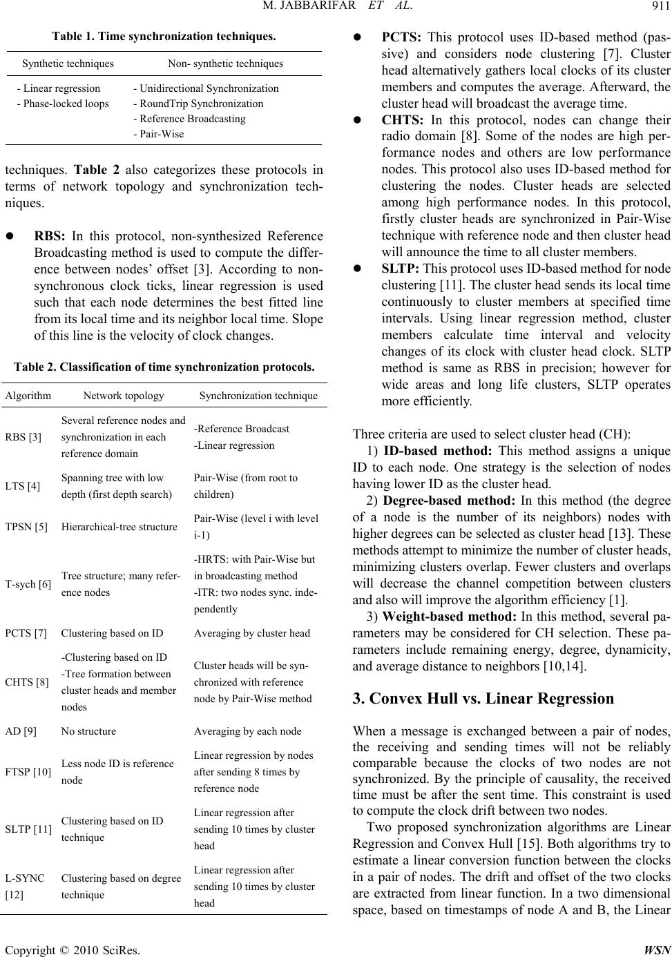

M. JABBARIFAR ET AL. 911
Table 1. Time synchronization techniques.
Synthetic techniques Non- synthetic techniques
- Linear regr e ss io n
- Phase-locked loops
- Unidirectional Synchronization
- RoundTrip Synchronization
- Reference Broadcasting
- Pair-Wise
techniques. Table 2 also categorizes these protocols in
terms of network topology and synchronization tech-
niques.
 RBS: In this protocol, non-synthesized Reference
Broadcasting method is used to compute the differ-
ence between nodes’ offset [3]. According to non-
synchronous clock ticks, linear regression is used
such that each node determines the best fitted line
from its local time and its neighbor local time. Slope
of this line is the velocity of clock changes.
Table 2. Classification of time synchronization protocols.
Algorithm Network topology Synchronization t echnique
RBS [3]
Several reference nodes and
synchronization in each
reference domain
-Reference Broadcast
-Linear regression
LTS [4] Spanning tree with low
depth (first depth search)
Pair-Wise (from root to
children)
TPSN [5] Hierarchical-tree structure Pair-Wise (level i with level
i-1)
T-sych [6] Tree structure; many refer-
ence nodes
-HRTS: with Pair-Wise but
in broadcasting method
-ITR: two nodes sync. inde-
pendently
PCTS [7] Clustering based on ID Averaging by cluster head
CHTS [8]
-Clustering based on ID
-Tree formation between
cluster heads and member
nodes
Cluster heads will be syn-
chronized with reference
node by Pair-Wise method
AD [9] No structure Averaging by each node
FTSP [10] Le ss node ID is reference
node
Linear regression by nodes
after sending 8 times by
reference node
SLTP [11] Clustering based on ID
technique
Linear regression after
sending 10 times by cluster
head
L-SYNC
[12]
Clustering based on degree
technique
Linear regression after
sending 10 times by cluster
head
 PCTS: This protocol uses ID-based method (pas-
sive) and considers node clustering [7]. Cluster
head alternatively gathers local clocks of its cluster
members and computes the average. Afterward, the
cluster head will broadcast the average time.
 CHTS: In this protocol, nodes can change their
radio domain [8]. Some of the nodes are high per-
formance nodes and others are low performance
nodes. This protocol also uses ID-based method for
clustering the nodes. Cluster heads are selected
among high performance nodes. In this protocol,
firstly cluster heads are synchronized in Pair-Wise
technique with reference node and then cluster head
will announce the time to all cluster members.
 SLTP: Thi s protoc ol uses I D-base d method for node
clustering [11]. The cluster head sends its local ti me
continuously to cluster members at specified time
intervals. Using linear regression method, cluster
members calculate time interval and velocity
changes of its clock with cluster head clock. SLTP
method is same as RBS in precision; however for
wide areas and long life clusters, SLTP operates
more efficiently.
Three criteria are used to select cluster head (CH):
1) ID-based method: This method assigns a unique
ID to each node. One strategy is the selection of nodes
having lower ID as the cluster head.
2) Degree-based method: In this method (the degree
of a node is the number of its neighbors) nodes with
higher degrees can be selected as cluster head [13]. These
methods attempt to minimize the number of cluster heads,
minimizing clusters overlap. Fewer clusters and overlaps
will decrease the channel competition between clusters
and also will improve the algorithm efficiency [1].
3) Weight-based method: In this method, several pa-
rameters may be considered for CH selection. These pa-
rameters include remaining energy, degree, dynamicity,
and average distance to neighbors [10,14].
3. Convex Hull vs. Linear Regression
When a message is exchanged between a pair of nodes,
the receiving and sending times will not be reliably
comparable because the clocks of two nodes are not
synchronized. By the principle of causality, the received
time must be after the sent time. This constraint is used
to compute the clock drift between two nodes.
Two proposed synchronization algorithms are Linear
Regression and Convex Hull [15]. Both algorithms try to
estimate a linear conversion function between the clocks
in a pair of nodes. The drift and offset of the two clocks
are extracted from linear function. In a two dimensional
space, based on timestamps of node A and B, the Linear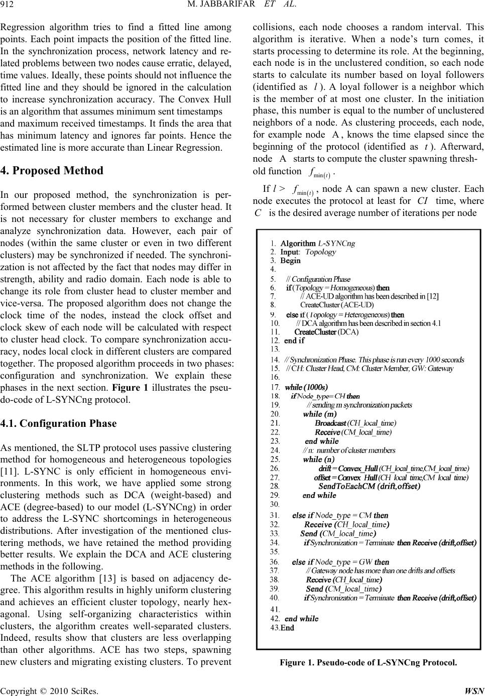

M. JABBARIFAR ET AL. 912
Regression algorithm tries to find a fitted line among
points. Each point impacts the position of the fitted line.
In the synchronization process, network latency and re-
lated problems between two nodes cause erratic, delayed,
time values. Ideally, these points should not influence the
fitted line and they should be ignored in the calculation
to increase synchronization accuracy. The Convex Hull
is an algorithm that assumes minimum sent timestamps
and maximum received timestamps. It finds the area that
has minimum latency and ignores far points. Hence the
estimated line is more accurate than Linear Regression.
4. Proposed Method
In our proposed method, the synchronization is per-
formed between cluster members and the cluster head. It
is not necessary for cluster members to exchange and
analyze synchronization data. However, each pair of
nodes (within the same cluster or even in two different
clusters) may be synchronized if needed. The synchroni-
zation is not affected by the fact that nodes may differ in
strength, ability and radio domain. Each node is able to
change its role from cluster head to cluster member and
vice-versa. The proposed algorithm does not change the
clock time of the nodes, instead the clock offset and
clock skew of each node will be calculated with respect
to cluster head clock. To compare synchronization accu-
racy, nodes local clock in different clusters are compared
together. The proposed algorithm proceeds in two phases:
configuration and synchronization. We explain these
phases in the next section. Figure 1 illustrates the pseu-
do-code of L-SYNCng protocol.
4.1. Configuration Phase
As mentioned, the SLTP protocol uses passive clustering
method for homogeneous and heterogeneous topologies
[11]. L-SYNC is only efficient in homogeneous envi-
ronments. In this work, we have applied some strong
clustering methods such as DCA (weight-based) and
ACE (degree-based) to our model (L-SYNCng) in order
to address the L-SYNC shortcomings in heterogeneous
distributions. After investigation of the mentioned clus-
tering methods, we have retained the method providing
better results. We explain the DCA and ACE clustering
methods in the following.
The ACE algorithm [13] is based on adjacency de-
gree. This algorithm results in highly uniform clustering
and achieves an efficient cluster topology, nearly hex-
agonal. Using self-organizing characteristics within
clusters, the algorithm creates well-separated clusters.
Indeed, results show that clusters are less overlapping
than other algorithms. ACE has two steps, spawning
new clusters and migrating existing clusters. To prevent
collisions, each node chooses a random interval. This
algorithm is iterative. When a node’s turn comes, it
starts processing to determine its role. At the beginning,
each node is in the unclustered condition, so each node
starts to calculate its number based on loyal followers
(identified as l). A loyal follower is a neighbor which
is the member of at most one cluster. In the initiation
phas e, this numb er is equal to the number of unclustered
neighbors of a node. As clustering proceeds, each node,
for example node

, knows the time elapsed since the
beginning of the protocol (identified as t). Afterward,
node

starts to compute the cluster spawning thresh-
old functi o n

min t
f.
If l >

min t
f, node A can spawn a new cluster. Each
node executes the protocol at least for CI time, where
C is the desired average number of iterations per node
Figure 1. Pseudo-code of L-SYNCng Protocol.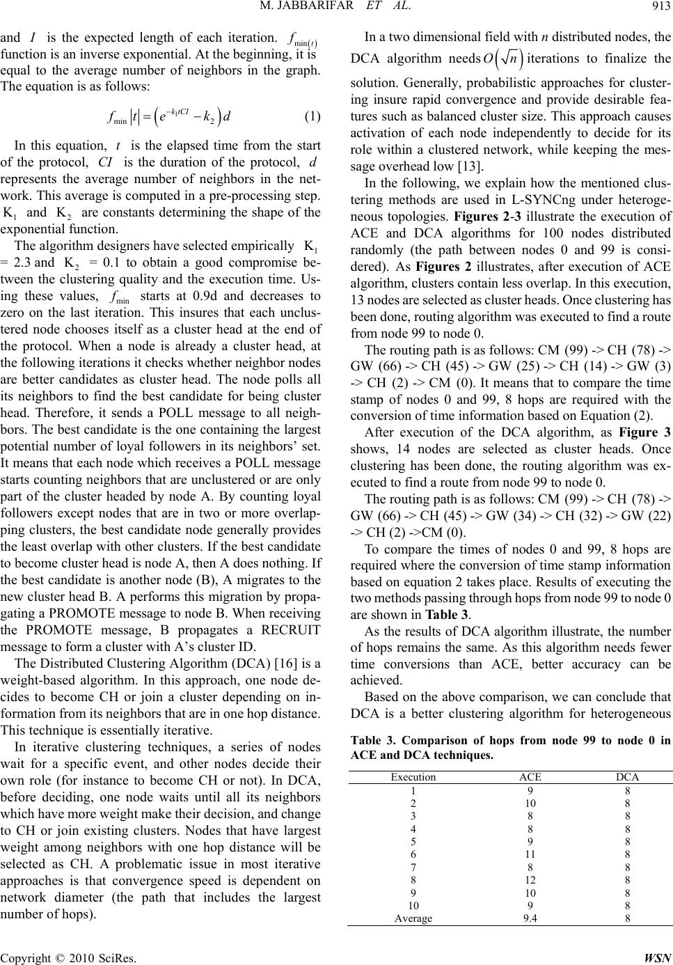

M. JABBARIFAR ET AL. 913
and
I
is the expected length of each iteration.

min t
f
function is an inverse exponential. At the beginning , it is
equal to the average number of neighbors in the graph.
The equation is as follows:

1
min 2
ktCI
f
te kd

 (1)
In this equation, t is the elapsed time from the start
of the protocol, CI is the duration of the protocol, d
represents the average number of neighbors in the net-
work. This average is computed in a pre-processing step.
1
K and 2 K are constants determining the shape of the
exponential functio n.
The algorithm designers have selected empirically 1 K
= 2.3 and 2 K = 0.1 to obtain a good compromise be-
tween the clustering quality and the execution time. Us-
ing these values, min
f
starts at 0.9d and decreases to
zero on the last iteration. This insures that each unclus-
tered node chooses itself as a cluster head at the end of
the protocol. When a node is already a cluster head, at
the following iterations it checks wheth er neighbor nodes
are better candidates as cluster head. The node polls all
its neighbors to find the best candidate for being cluster
head. Therefore, it sends a POLL message to all neigh-
bors. The best candidate is the one containing the largest
potential number of loyal followers in its neighbors’ set.
It means that each node which receives a POLL message
starts counting neighbo rs that are unclustered or are only
part of the cluster headed by node A. By counting loyal
followers except nodes that are in two or more overlap-
ping clusters, the best candidate node generally provides
the least overlap with other clusters. If the best candidate
to become cluster head is node A, then A does nothing. If
the best candidate is another node (B), A migrates to the
new cluster head B. A performs this migration by propa-
gating a PROMOTE message to node B. When receiving
the PROMOTE message, B propagates a RECRUIT
message to form a cluster with A’s cluster ID.
The Distributed Clustering Algorithm (DCA) [16] is a
weight-based algorithm. In this approach, one node de-
cides to become CH or join a cluster depending on in-
forma t i on f r o m i t s ne i g h b o r s t ha t a re in on e h o p di s t a n c e .
This technique is essentially iterative.
In iterative clustering techniques, a series of nodes
wait for a specific event, and other nodes decide their
own role (for instance to become CH or not). In DCA,
before deciding, one node waits until all its neighbors
which ha ve m ore weig ht m ake t heir decisio n, a nd c hange
to CH or join existing clusters. Nodes that have largest
weight among neighbors with one hop distance will be
selected as CH. A problematic issue in most iterative
approaches is that convergence speed is dependent on
network diameter (the path that includes the largest
number of hops).
In a two di mensional fi el d wi th n dist ributed no des, the
DCA algorithm needs


Oniterations to finalize the
solution. Generally, probabilistic approaches for cluster-
ing insure rapid convergence and provide desirable fea-
tures such as balanced cluster size. This approach causes
activation of each node independently to decide for its
role within a clustered network, while keeping the mes-
sage overhead low [ 13] .
In the following, we explain how the mentioned clus-
tering methods are used in L-SYNCng under heteroge-
neous topologies. Figures 2-3 illustrate the execution of
ACE and DCA algorithms for 100 nodes distributed
randomly (the path between nodes 0 and 99 is consi-
dered). As Figures 2 illustrates, after execution of ACE
algorithm, clusters contain less overlap. In this execution,
13 nodes are selected as cluster heads. Once clusteri ng has
been done, r o u ti ng algorithm was executed to find a route
from node 99 to node 0.
The routing path is as follows: CM (99) -> CH (78) ->
GW (66) -> CH (45) -> GW (25) -> CH (14) -> GW (3)
-> CH (2) -> CM (0). It means that to compare the time
stamp of nodes 0 and 99, 8 hops are required with the
conversion of time informati on based on Equati on (2 ).
After execution of the DCA algorithm, as Figure 3
shows, 14 nodes are selected as cluster heads. Once
clustering has been done, the routing algorithm was ex-
ecuted to find a route from node 99 to node 0.
The routing path is as follows: CM (99) -> CH (78) ->
GW (66) -> CH (45) -> GW (34) -> CH (32) -> GW (2 2 )
-> CH (2) ->CM (0).
To compare the times of nodes 0 and 99, 8 hops are
required where the conversion of time stamp information
based on equation 2 takes place. Results of executing the
two me thods passing thr ough hops fr om node 99 to node 0
are shown in Table 3.
As the results of DCA algorithm illustrate, the number
of hops remains the same. As this algorithm needs fewer
time conversions than ACE, better accuracy can be
achieved.
Based on the above comparison, we can conclude that
DCA is a better clustering algorithm for heterogeneous
Table 3. Comparison of hops from node 99 to node 0 in
ACE and DCA techniques.
Execution ACE DCA
1 9 8
2 10 8
3 8 8
4 8 8
5 9 8
6 11 8
7 8 8
8 12 8
9 10 8
10 9 8
Average 9.4 8

M. JABBARIFAR ET AL. 914
Figure 2. Using ACE as a clustering in L-SYNCng.
Figure 3. Using DCA as a clustering in L-SYNCng.
topologies. Therefore, this algorithm can be used by
L-SYNCng in het e r ogeneous t op ol o gi es.
4.2. Synchronization Phase
In this phase, each cluster head starts to broadcast a
synchronization pack et including its identity number and
local time. Each cluster member receives this packet and
sends an acknowledgment to the cluster head.
The cluster head waits to receive all ACK messages,
as shown in Figure 4. Thus four timestamps (tcs, tmr, tms,
tcr) are generated for each ACK. If a cluster member re-

M. JABBARIFAR ET AL. 915
Figure 4. Synchronization packets between CH and CMs.
CH starts synchronization.
plies immediately to the cluster head, tmr would be equal
to tms. A cluster member can delay as long as it wants.
The precision will decrease if the delay between tcs and
tcr increases. Cluster head has tcs, tms and tcr.
To determine tmr it is eno ugh to have the minimum de-
lay between tmr and tms . The minimum delay can be esti-
mated by the cluster head for each cluster member at the
end of broadcasting, based on the history of each cluster
member’s behavio r [1 7] .
The cluster head will broadcast a next synchronization
packet. After sending m packets, CH will derive an equa-
tion of the form Y=aX+b where a and b are spe-
cific for each cluster member. Eventually, the cluster
head sends all a and b to each cluster member.
As mentioned, Figure 5 shows that the convex hull
technique can be used to derive lower and upper bounds
on the local time of a remote node. In this case, each
cluster head can generate a two dimensional graph for
each cluster member after sending m packets. The x -axis
and y-axis dimensions are local times of cluster member
and cluster head repetitively. Thus, each cluster member
has two clouds formed by lower-bound and upper-bond
samples. Unlike liner regression that tends to average all
the individual samples, this technique ignores average
values and accounts for the samples with minimal or
maximal error [2,14].
Table 4 shows the nu mber of messages used in the syn-
chronization phase for SLTP, L-SYNC and L-SYNCng,
m, c and n indicates number of synchronization pack-
ets , number of cluster heads and number of cluster mem-
bers respectively. It i s obvious that the li near regression
Figure 5. Convex Hull method.
Table 4. Number of transmitted messages for the following
algorithms.
Algorithms Number of messages
SLTP C * m
L-SYNC C * m
L_SYNCng C * [(1+n) * m+ n]
Figure 6. Synchronization packets between CH and CMs.
CM starts synchronization.
used in SLTP and L-SYNC has fewer messages.
Another solution that can be discussed is to start
sending synchronization packets by cluster members.
Figure 6 shows this solution. With this solution, each
cluster member sends m synchronization packet to clus-
ter head and then receives m ACK messages. However,
the number of messages in this method is 2*m*n and has
more overhead rather than first solution, although this
solution has better scalability.
Between clusters, there are some nodes that receive
timing packets from more than one group head; these are
called gateways. Synchronization can be performed pe-
riodically at specific time intervals. But, if a node needs
to be synchronized within these time intervals, it can
broadcast a message for synchronization.
Any group head that receives this message will start to
send its local time and ID. In the example shown in Fig-
ure 7, after executing the algorithm in cluster heads CH1
to CH2, nodes belonging to each group head will re-
ceive a and b. If two nodes such as CM1 and CM2,
that are the members of a cluster, want to communicate
with each other, it is sufficient to send their a and b
parameters to each other, and using the following equa-
tions they can convert their clocks. In a case where two
nodes are not members of a cluster, they can also be
synchronized. For instan ce, if nodes CM1 and CM3 w ant
to be synchronized, it is enough to calculate a and b
Figure 7. Synchronization of two nodes of two far clusters.

M. JABBARIFAR ET AL. 916
parameters using Equation (2), in the path between each
two nodes, in an appropriate route between nodes CM1
and CM3. We have proposed a routing algorithm be-
tween these nodes. Afterward, clock conversion will be
done in each existing hop in the route path. Since con-
version error in each hop will be added to the total error
rate, the synchronization error increases with the number
of hops. Consequently, clustering based on larger number
of neighbors helps to shorten the route between two
nodes, in order to perform fewer conversions and reduce
the synchronization error rate.
11
12
1CH1CM1
2CH2CM2
C+
C+
ah b
ah b


：h
：h12
221
CM CM
11
abb
hh
aa





(2)
5. Results
To assess our synchronization protocol, we used the NS
2.31 simulator under the Linux operating system. We
describe the simulation setup and configuration in detail
in Subsection 5.1. Afterward, we selected SLTP [2] and
L-SYNC [12] to compare our simulation results based on
accuracy in terms of time and number of hops. We dis-
cuss our comparison in detail in Subsection 5.2.
5.1. Simulation Setup
To evaluate the proposed algorithm, it is required to con-
sider several clocks, one for each node. To simulate sev-
eral nodes’ clocks on a system, a real time system was
used, so that for each node’s clock, one specific drift and
one specific offset were selected.
Drift and offset are determined by a random function,
between two identified values of max_drift and max_
offset, such that nodes’ clocks are computed with the
following equations. In our simulations, the worst cases
for drift and offset have been considered. Simulation
parameters are shown in Table 5.
When a node wants to be synchronized with another
node, a packet is broadcast to form an optimized route
between two nodes. In the return route, the required
conversions are done. In each execution turn, different
Table 5. Simulation parameters values.
Subject Value
Number of synchronization packets 10
Time intervals between synchronization packets 1s
Synchronization period 1000s
Max. offset 1s
Max. drift 0.0001s
Simulation dura t ion 10262s
routes between source and target will be selected, each
experiment will be iterated 10 times and the results are
averaged. Our simulation is done for two different to-
pologies, heterogeneous and homogeneous. In homoge-
neous topology we use 100 nodes in 1000*1000 square
meters where each node has 100 meters range in a regu-
lar layout, and in heterogeneous topology the configura-
tion is similar except that the nodes coordinates are ran-
domly uniform.


* 3time nodecurrent timedriftoffset
5.2. Simulation Results and Comparison
We simulated our work in two environments: noisy and
noiseless. Each environ ment was tested with two topolo-
gies: homogeneous and heterogeneous. Figure 8 depicts
the average error versus simulation time in noiseless
homogeneous environment. It shows that as time passes
the average error rate of L-SYNCng increases less than
with the others.
Figure 9 depicts our second simulation in noiseless
heterogeneous topology. It shows that as time passes the
average error rate of L-SYNCng increases gradually,
while for the other protocols it increases more rapidly.
We have repeated the two previous simulations innoi-
sy environment where packets may arrive to destination
with considerable delay. Figures 10-11 depict our simu-
lation results. As we mentioned, in L-SYNC the protocol
synchronization algorithm is based on linear regression
technique. Linear regression can be influenced particu-
larly by unreliable data which are far from the fitted line.
Figures 12-13 summarize L-SYNC and L-SYNCng
general behavior in each different environment.
Figure 8. Comparison of L-SYNCng, L-SYNC and SLTP
error versus time in homogeneous topology and noiseless
environment.

M. JABBARIFAR ET AL. 917
Figure 9. Comparison of L-SYNCng, L-SYNC and SLTP
error versus time for heterogeneous topology and noiseless
environment.
Figure 10. Comparison of L-SYNCng, L-SYNC and SLTP
error versus time forhomogeneous topology and noisy en-
vironment.
Figure 11. Comparison of L-SYNCng, L-SYNC and SLTP
error versus time for heterogeneous topology and noisy
environment.
Figure 12. L-SYNCng behavior in different environment.
Figure 13. L-SYNC behavior in different environment.
6. Conclusions and Future Work
L-SYNCng is a reliable and efficient protocol for time
synchronization in Wireless Sensor Networks. This pro-
tocol uses degree-based and weight-based clustering in
heterogeneous and homogeneous topologies respectively.
Using these clustering methods, L-SYNCng can reduce
the number of hops in time synchronization process of
two specific nodes which are in different clusters.
Moreover, L-SYNCng uses convex hull method to
calculate clock offset and skew in each cluster. Therefore,
it is capable to compute skew and offset intervals be-
tween each node and its corresponding head cluster. In
other words, it can estimate the local time of remote
nodes in the future and past. To estimate the local time
for remote nodes, firstly a routing algorithm is used and
afterward a conversion is performed in each hop. Simu-
lation results illustrate that the convex hull method can
increase efficiently the synchronization accuracy in noisy
environments. As dynamic sensor networks might be
indispensable in the future, we are going to apply
LSYNCng to these environments where nodes change

M. JABBARIFAR ET AL. 918
their status during time.
7. References
[1] H. Chan and A. Perrig, “ACE: An Emergent Algorithm
for Highly Uniform Cluster Formation,” Wireless
Sensor Networks, Vol. 2920, January 2004, pp. 154-
171.
[2] www.vs.inf.ethz.ch/publ/papers/wsn-time-boo k.pdf
[3] J. Elson, L. Girod and D. Estrin, “Fine-Grained Network
Time Synchronization, Using Reference Broadcasts,”
Proceedings of the 5th Symposium on Operating Systems
Design and Implementation, Vol. 36, No. SI, Winter
2002, pp. 147-163.
[4] J. V. Greunen and J. Rabaey, “Lightweight Time Syn-
chronization for Sensor Networks,” Proceedings of the
2nd ACM International Conference on Wireless Sensor
Networks and Applications, 2003, pp. 11-19.
[5] H. Dai and R. Han, “TSync: A Lightweight Bidirectional
Time Synchronization Service for Wireless Sensor Net-
works,” ACM SIGMOBILE Mobile Computing and
Communications Review Archive, Vol. 8, No. 1, January
2004, pp. 125-139.
[6] S. Ganeriwal, R. Kumar and M. B. Srivastava, “Tim-
ing-Sync Protocol for Sensor Networks,” Proceedings of
the 1st International Conference on Embedded Net-
worked Sensor Systems, 2003, pp. 138-149.
[7] Md. Mamun-Or-Rashid, C. S. Hong and C. Hyung, “Pas-
sive Cluster Based Clock Synchronization in Sensor
Network,” Advanced Industrial Conference on Telecom-
munications/Service Assurance with Partial and Inter-
mittent Resources Conference/E-Learning on Telecom-
munications Workshop (AICT/SAPIR/ELETE’05), July
2005, pp. 340-345.
[8] H. Kim, D. Kim and S. Yoo, “Cluster-Based Hierarchical
Time Synchronization for Multi-Hop Wireless Sensor
Networks,” 20th International Conference on Advanced
Information Networking and Applications, Vol. 2, April
2006, pp. 318-322.
[9] K. Römer, “Time Synchronization and Localization in
Sensor Networks,” Ph.D. Thesis, No. 16106, ETH Zurich,
Switzerland, June 2005.
[10] M. Maroti, B. Kusy, G. Simon and A. Ledeczi, “The
Flooding Time Synchronization Protocol,” Proceedings
of the 2nd International Conference on Embedded Net-
worked Sensor Systems, SenSys, November 2004.
[11] S. N. Gelyan, A. N. Eghbali, L. Roustapoor, S. A. Ya-
hyavi, F. Abadi and M. Dehghan, “Scalable Lightweight
Time Synchronization, Protocol for Wireless Sensor
Network,” International Conference on Mobile Ad-Hoc
and Sensor Networks, Beijing, December 2007,
pp.536-547.
[12] M. Jabbarifar, A. S. Sendi, H. Pedram, M. Dehghan and
M. Dagenais, “L-SYNC: Larger Degree Clustering Based
Time-Synchronisation for Wireless Sensor Network,”
Eighth ACIS International Conference on Software En-
gineering Research, Management and Applications,
Montreal, 2010.
[13] O. Younis, M. Krunz and S. Ramasubramanian,
“Clustering in Wireless Sensor Networks: Recent De-
velopments and Deployment Challenges,” IEEE Net-
work Magazine, Vol. 20, No. 3, May 2006, pp. 20-25.
[14] B. Poirier, R. Roy and M. Dagenais, “Accurate Offline
Synchronization of Distributed Traces Using Kernel-
Level Events,” ACM SIGOPS Operating Systems Review,
Vol. 44, No. 3, July 2010, pp. 75-87.
[15] A. Duda, G Harrus, Y. Haddad and G. Bernard, “Esti-
mating Global Time in Distributed Systems,” Proceed-
ings of the 7th International Conference on Distributed
Computing Systems, Berlin, Vol. 18, 1987.
[16] S. Basagni, “Distributed Clustering Algorithm for Ad
Hoc Networks,” International Symposium on Parallel
Architectures, Algorithms and Networks (ISPAN’99),
1999, pp. 310-315.
[17] L. M. Sichitiu and C. Veerarittiphan, “Simple, Accurate
Time Synchronization for Wireless Sensor Networks,”
IEEE Wireless Communications and Networking Confe-
rence (WCNC’03), Vol. 2, March 2003, pp. 1266-1273.