 Journal of Mathematical Finance, 2013, 3, 392-400 http://dx.doi.org/10.4236/jmf.2013.33040 Published Online August 2013 (http://www.scirp.org/journal/jmf) A Liability Tracking Approach to Long Term Management of Pension Funds Masashi Ieda1, Takashi Yamashita2, Yumiharu Nakano 1 1Graduate School of Innovation Management, Tokyo Institute of Technology, Tokyo, Japan 2The Government Pension Investment Fund, Tokyo, Japan Email: ieda@craft.titech.ac.jp Received May 28, 2013; revised July 2, 2013; accepted July 11, 2013 Copyright © 2013 Masashi Ieda et al. This is an open access article distributed under the Creative Commons Attribution License, which permits unrestricted use, distribution, and reproduction in any medium, provided the original work is properly cited. ABSTRACT We propose a long term portfolio management method which takes into account a liability. Our approach is based on the LQG (Linear, Quadratic co st, Gaussian) control problem framework and then the optimal po rtfolio strategy hedges the liability by directly tracking a benchmark process which represents the liability. Two numerical results using em- pirical data published by Japanese organizations are served: simulations tracking an artificial liability and an estimated liability of Japanese organization. The latter one demonstrates that our optimal portfolio strategy can hedge his or her liability. Keywords: Pension Fund Management; Long Term Portfolio Optimization; Quadratic Hedging; Stochastic Optimal Control; Hamilton-Jacobi-Bellman Equations; LQG Control 1. Introduction In the management of pension funds, a long term portfo- lio strategy taking into account a liability is one of the most significant issues. The main reason is the demo- graphic changes in the developed countries: if the work- ing-age population is enough to provide for old age, the liability is a minor issue in the portfolio management of pension funds. Sin ce the life expectancy has increased in recent decades, it becomes insufficient to provide for old age. Furthermore, the low birth rate continues and drives up this problem for decades. Thus pension funds face a challenging phase to construct long term portfolio strate- gies which hedge their liabilities. A lot of pension funds except a few ones [1] determine their portfolio strategies by the traditional single time period mean variance approach which excludes an eva- luation of a liability. Its intuitive criterion attracts man- agers of pension funds. However the single time period approach is unsuitable for a long term portfolio manage- ment in the sense that it is unable to change the strategy excepting the initial time. The multi time period ap- proach which arrows the change of the strategy has a problem that the computational complexity grows expo- nentially. Hence if we employ this approach, we are usu- ally unable to ob tain the optimal p ortfo lio strategy in rea- listic time. Therefore the aim of this paper is to propose a long term portfolio strategy which 1) involves an evaluation of a liability, 2) admits changes of the strategy at any time, and 3) is obtained in realistic time. To tackle this problem, we employ the LQG (Linear, Quadratic cost, Gaussian) control problem (see, e.g., Fleming and Rishel [2]). The LQG control problem is a class of stochastic control problem and is able to provide the control mini- mizing the mean square error of a benchmark process and a controlled process. Roughly speaking our tactic is that we compute the optimal portfolio strategy with the benchmark process which represents the liability. Then we can track the liability by using our optimal portfolio strategy. Although it is difficult to obtain the solution of stochastic control problem in general, the LQG control problem has the analytical solutio n which assu res that we are able to obtain the solu tion in realistic time and thus it meets our purpose. A continuous time stochastic control approach is one of the most popular methods to obtain the suitable long term portfolio strategy. The literatu re abou t this appro ach is quite rich. The papers treating the management of pen- sion funds are, for instance, as follows: Deelstra et al. [3] and Giacinto et al. [4] discuss the portfolio management for pension funds with a minimum guarantee; Menoncin and Scaillet [5] and Gerrard et al. [6] deal with the pen- C opyright © 2013 SciRes. JMF 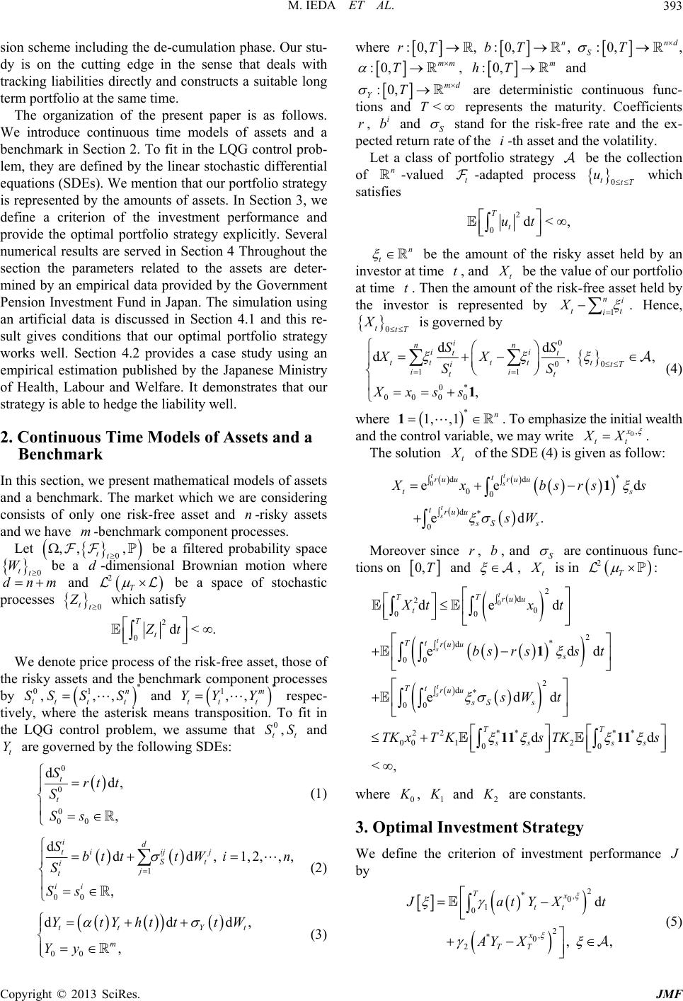 M. IEDA ET AL. 393 sion scheme including the de-cumulation phase. Our stu- dy is on the cutting edge in the sense that deals with tracking liabilities directly and constructs a suitable long term portfolio at the same time. The organization of the present paper is as follows. We introduce continuous time models of assets and a benchmark in Section 2. To fit in the LQG control prob- lem, they are defined by the linear stochastic differential equations (SDEs). We mention that our portfolio strategy is represented by the amounts of assets. In Section 3, we define a criterion of the investment performance and provide the optimal portfolio strategy explicitly. Several numerical results are served in Section 4 Throughout the section the parameters related to the assets are deter- mined by an empirical data provided by the Government Pension Investment Fund in Japan. The simulation using an artificial data is discussed in Section 4.1 and this re- sult gives conditions that our optimal portfolio strategy works well. Section 4.2 provides a case study using an empirical estimation published by the Japanese Ministry of Health, Labour and Welfare. It demonstrates that our strategy is able to hedge the liability well. 2. Continuous Time Models of Assets and a Benchmark In this section, we present mathematical models of assets and a benchmark. The market which we are considering consists of only one risk-free asset and -risky assets and we have -benchmark component processes. n m Let 0t be a filtered probability space be a -dimensional Brownian motion where and be a space of stochastic processes which satisfy ,, , t 0d m 2T 0 tt Z tt W dn 2 0d<. T t Zt We denote price process of the risk-free asset, those of the risky assets and the benchmark component processes by , and respec- tively, where the asterisk means transposition. To fit in the LQG control problem, we assume that , and are governed by the follow ing SDEs: 0 t S * 1,, n tt t SS S * 1,, m tt t YY Y 0 t St S t Y 0 0 0 00 dd, , t t Srt t S Ss (1) 1 00 ddd, 1,2,,, , id iijj tSt ij t ii Sbt tt Win S Ss (2) 00 dd , tt Y m YtYhttt Yy :0,rT, :0, n bT, :0, nd ST , d, t W (3) where :0 ,mm T , :0, m hT and :0,T md Y nd <T are deterministic continuous func- tions a r r, i b and S eps resents the maturity. Coefficient pected return rate o stand fo-free rar the riskte and the ex- ss of ed f the i-th asset and the volatility. Let a claportfolio strategy be the collection of n-valu t -adapted process 0 ttT u which satisfies 2 0d<, T t ut n t nvestor at tbe the amount of the risky asset held by an iime , and tt ount be the vae of our portfolio . Thene am of the risree asset held by th lu k-fat time t e invest th or is represented by 1 tt i Xni . Hence, 0 ttT X is govrned bye 0 0 11 0* dd d , , i nn ii tt 0 0000 , tt t tT Xx where . To emphasize the initial w and thmay write tt i ii tt SS XX SS ss 1 (4) * 1, ,1n 1 e control variable, we ealth 0,x tt XX . The solution t of the SDE (4) isw: s given as follo d d 0 t t ru u 0* d 00 ee d t sruu t * ed . t s tru u sSs xbsrss sW 1 Moreover since , and r, bS are continuous func- tions on 0,T and , t is in 2T : 0 2 d 2 * d 00 2 d* 00 2 2**** 00 12 00 ed edd edd dd <, t t s t s TT ru u Tt ru u s Tt ru u sS s TT ss ss bs rss t sW t TK xTKsTKs 20 00 d t Xtx t 1 11 11 where 0 , 1 and 2 are constants. 3. Optimal In v es t me nt Strategy inehen erformance We def t criterioof investment p by *, Tx 2 2 , *0 2 d , , x TT 0 1 0tt at YXt AY X ( ) 5 Copyright © 2013 SciRes. JMF 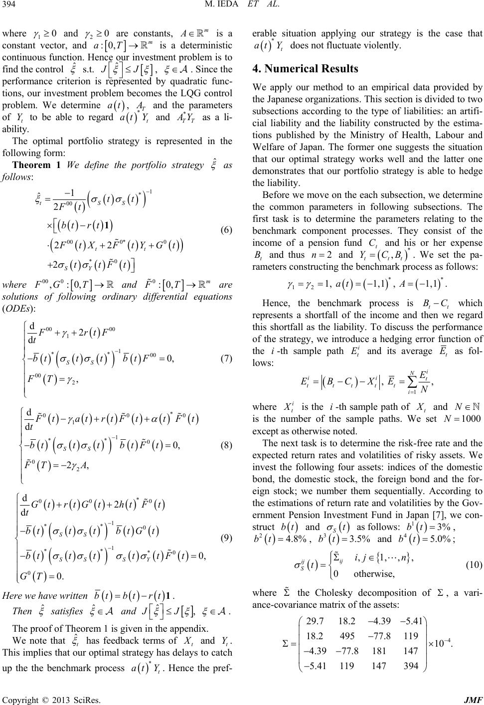 M. IEDA ET AL. 394 are constants, m where 10 and 20 is a constan, ant vectord :0 Hence,m aT our invest is contin ction.ment find thel a determin pistic roblem is to uous fun controˆ s.t. ˆ JJ , by . Sinc quadratic f LQG co e the perforunc- mance cri ur inveterion is re t probl e presented at, tions, ostmenem becomes the ntrol problem. We determinT t and the parameters of t Y to be able to regard * at Y and * TT Y as a li- ability. The optimal portfolio strategy is represented in the following form: Theorem 1 We define ptfolio strategy ˆ theor as follows: 1 * 00 1 ˆ2 tSS tt Ft bt rt 00 0* 0 *0 22 2 tt SY tXFtYG t ttFt where 1 (6) 00 0 ,:0,FG T and 0:0,FT nary differential equations m are solutions (ODEs): of following ordi 1 ** 00 00 d 0, SS bt ttbtF (7) 00 00 1 2 d2 , FrtF t FT * 00 1 1 ** 0 02 d d 0, 2, SS 0 tatrtFt t t btttbtF t FT A (8) Ft * 00 0 1 ** 0 1 ** *0 0 d2 d 0, 0. SS SS SY Gt rtGthtFt t btttbtG t btttttF t GT (9) Here we have written btbt rt1. Then ˆ satisfies ˆ and ˆ J , . The proof of Theorem 1 is given in the appendix. We note that ˆt has feedback terms of t and mal strategy has to catch up the the benchmark process . Hence the pref- ertuying otegy is the case th 4. R pirical section cial liabted by the estima- nistry of Health, Labour and er one suggests the situation t Y. This implies that our optidelays * t atY able siation applur straat * at Y tdoes not fluctuate violently. Numerical esults We apply our method to an em data provided by the Japanese organizations. This is divided to two subsections according to the type of liabilities: an artifi- ility and the liability construc tions published by the Mi Welfare of Japan. The form that our optimal strategy works well and the latter one demonstrates that our portfolio strategy is able to hedge the liability. Before we move on the each subsection, we determine the common parameters in following subsections. The first task is to determine the parameters relating to the benchmark component processes. They consist of the income of a pension fund t C and his or her expense t B and thus 2n and * ,B. We set the pa- ra ttt YC meters constructing the benchmark process as follows: ** 12 1, 1,1, 1,1.at A Hence, the benchmark process is tt BC which represents a shortfall of the come and then we regard tis shortfall asliabilits the performance of the strategy, we introduce a hedging error function of the i-th sample path iand its average in h the y. To discus t E t E as fol- lows: 1 , , N ii tt ttt i E EBCXE N where i t i t is the i-th sample path of t and N is the number of the sample paths. We set 1000N except as otherwise noted The . next task is to determine the risk-free rate and the expected return rates and volatilities of risky assets. We invest the following four assets: indices of the domestic he ondhe for ording to the Gov- bond, tdomestic stock, the foreign b and t- eign stock; we number them sequentially. Acc the estimations of return rate and volatilities by ernment Pension Investment Fund in Japan [7], we con- struct bt and St as follows: 13%bt, 24.8%bt, 33.5%bt and 45.0%bt; ,1,,, 0 otherwise, ij ij S ij n t (10) where the Cholesky decomposition of , a vari- ance-coance mf the assets: 29.7 4.39 variatrix o 4 10 . 18.2 5.41 18.249577.8 119 4.3977.8 181147 5.41 119147394 Copyright © 2013 SciRes. JMF 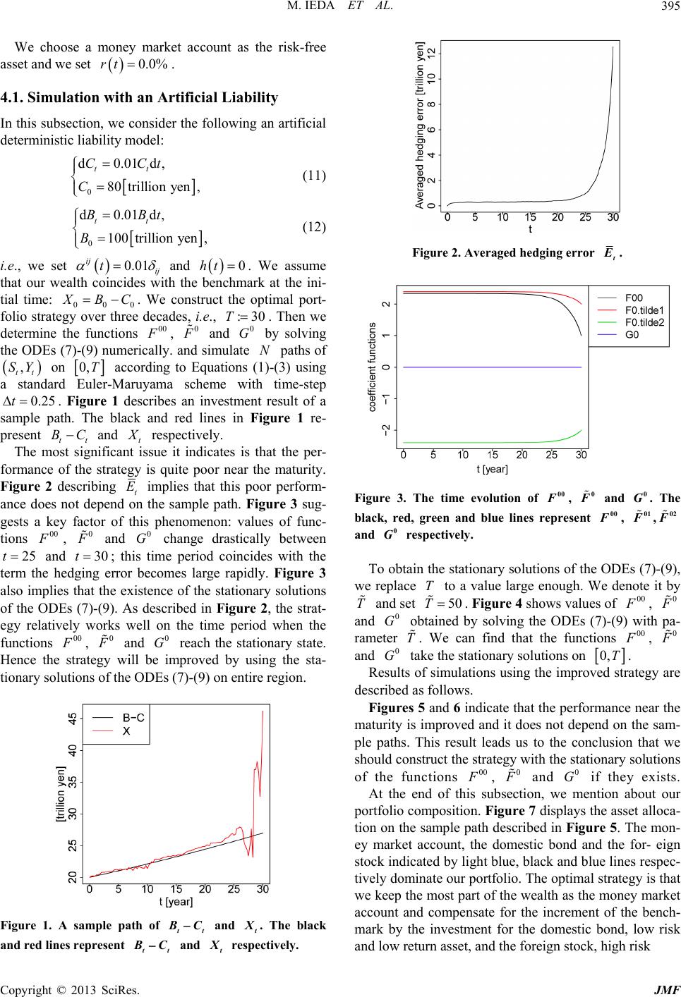 M. IEDA ET AL. 395 We choose a money market account as the risk-free asset and we set 4.1. Simulation with an Artificial Liability In th is subsec tion, we con sider the following an artificial deterministic liability model: (11) i.e., we set 0.0%rt. 0 0.01d, 80trillion yen, tt C dCCt 01 00trillionyen, tt B (12) d0.01d,BBt 0.01 ij t ij wealth coincides wi 000 and . We assume that our th the tial time: 0ht benchmark at the ini- BC. We over three deca functions 00 constptimal port- folio strategydes,. Then we determ ruct the o i.e., T:30 ine the , 0 d simulate and 0 G by solving the ODEs paths of (7)-(9) numerically. anN , tt SY on 0,T accordin Figure 1 de g to E (1)-(3) using a standard Euler-Maruyama scheme with time-step 0.25t . scribes an investment result of a sample path. The black and red linesure 1 re- present tt BC and t quations in Fig respectively. The most significant issue it indicates is that the per- formrategy is quite poor near the maturity. Figure 2 describing ance of the st t E implies that this poor perform- a not depend on the sample path. Figure 3 sug- gests a key factor of this phenomenon: values of func- tions 00 nce does , 0 and 0 change drastically between G 25 and 30t; this time period coincides with the term the hedging error becomes large rapidly. Figure 3 also implies that the existence of the stationary solutions of the ODEs (7)-(9). As described in Figure 2, the strat- egy relatively works well on the time period when the functi 00 t ons , 0 an0 G reach the stationary state. H the st will be improved by using the sta- tionary solutions of the ODEs (7)-(9) on entire region. d ence rategy Figure 1. A sample path of and tt BCt Figure 2. Averaged hedging error t . Figure 3. . The lack, red The time evolution of F, F and , green and blue lines represent 00 0 0 G 01 b00 F, ,02 and respectively. To obtain the stationary solutions of the ODEs (7)-(9), we replace to a value large enough. We denote it by and set 0 G T TT 50 . Figure 4 shows values of 00 , 0 pa-and ram 0 G eter obtained by solving the ODEs (7)- can find that the functions (9) with 00 T . We , 0 and 0 G take the stationary solutions on 0,T. proved strategy are Results of simulations using the im described as follows. Figures 5 and 6 indicate that the performance near the maturity is improved and it does not depend on the sam the oncth the ol - ple paths. This result leads us to clusion at we should construct the strategy with stationary sutions of the functions 00 , 0 and 0 G ifeyxi. Ate end of this s th ests thbn, ntion about our portfolio com tio st ed by ec th rke bench- md the foreign stock, h igh risk usectiowe me position. Figure 7 displays the asset alloca- n on the sample path described in Figure 5. The mon- ey market account, the domestic bond and the for- eign ock indicatlight blue, black and blue lines resp- tively dominate our portfolio. The optimal strategy is that we keep e most part of the wealth as the money mat account and compensate for the increment of the . The black and red lines represent tt and BCt ark by the investment for the domestic bond, low risk and low return asset, an resectively. p Copyright © 2013 SciRes. JMF 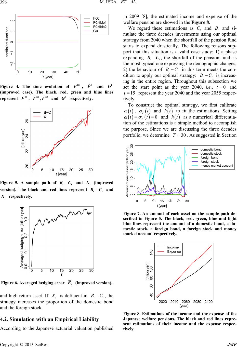 M. IEDA ET AL. 396 Figure 4. The time evolution of 00 F, 0 F and 0 G (improved case). The black, red, green and blue lines represent 00 F, 01 F,02 F and 0 G respectively. Figure 5. A sample path of tt BC and t (improved version). Tbl a red lin represent tt B he ackndesC and t respectively. gure 6. AveragedFi hedging error t (improved version). nd high return asset. If at is deficient in tt BC , the strategy increases the ption of the do and the foreign stock. 4.2. Simulation with an Empirical Liability According to the Japanese actuarial valuation published in 2009 [8], the estimated income and expense of the welfare pension are showed in the Figure 8. We regard these estimations as and and si- mulate the three decades investmenoptimal strategy from 2040 when the shortfall of the p fund starts to expand drastically. The following rs sup- port that this situation is a validdy: 1 a phase expanding ropormestic bond t C nts usi case stu t B g our ension eason ) tt BC , the shortfall ofpefund, is the mo st typical one expressing the dem; 2) the beha the nsion ographic changes viour oftt BC optima on. Th in this meets the con- dition to applyl strategy: increas- ing in the entire roughout twe 2 term h 0 our regi tt BC is is subsection set the start point as the year 40, i.e., 0t and 15t represent the year 2040 anhe year 2055 respec- d t tively. To construct the optimal strategy, we first calibrate t , Yt and ht to fit the estimations. Setting 0 Y tt and ht as a numerical differentia- plish cades tion of the estimations is a simple method to accom the purpose. Since we are discussing the three de portfolio, we determine 30T . As suggested in Section Figure 7. An amount of each asset on the sample path de- d in Figure 5. The black, red, green, blue and light blue lin scribe es represent the amount of a domestic bond, a do- m markc ntive estic stock, a foreign bond, a foreign stock and money et acout respecly. Figure 8. Estimations of the income and the expense of the Japanese welfare pensions. The black and red lines repre- sent estimations of their income and the expense respec- tively. Copyright © 2013 SciRes. JMF 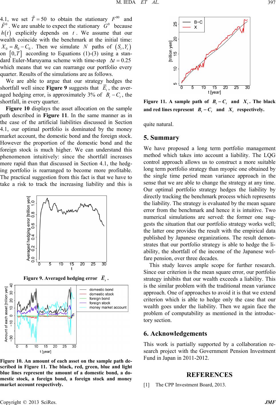 M. IEDA ET AL. 397 4.1, we set 50T to obtain the stationary 00 and 0 . We are unable to expect the stationary 0 G because ht explicitly depends on t. We assume that our wealth coincide with the benchmark at the initial time: 000 BC. Then we simute pathla Ns of , tt SY on 0,T Euler-according to Equations a sce-ste (1)-(3) using a p stan- 0.25 dardMaruyam heme with timt which means that we can rearrange our portfolio every quarter. Results of the simulations are as follows. We are able to argue that our strategy hedges the shortfall well since Figure 9 suggests that t E , the aver- aged hedging error, is approximately 3% oftt BC , the shortfall, in every quarter. Figure 10 displays the asset allocation on the sample path described in Figure 11. In the same manner as in the case of the artificial liabilities discussed in Section 4.1, our optimal portfolio is dominated by the money ncr ing p market account, the domestic bond and the foreign stock. However the proportion of the domestic bond and the foreign stock is much higher. We can understand this phenomenon intuitively: since the shortfall ieases more rapid than that discussed in Section 4.1,the hedg- ortfolio is rearranged to become more profitable. The practical suggestion from this fact is that we have to take a risk to track the increasing liability and this is Figure 9. Averaged hedging error t . Figure 10. An amount of each asset on the sample path de- scribed in Figure 11. The black, red, green, blue and light blue lines represent the amount of a domestic bond, a do- mestic stock, a foreign bond, a foreign stock and money market account respectively. Figure 11. A sample path of tt BC and t . The black and red lines represent tt BC and t resectively. quite natural. 5. Summary We have proposed a long term portfolio management method which takes into account a liability. The LQG control approach allows us to construct a more suitable long term portfolio strategy than myopic one obtained by the single time period mean variance approach in th d hence it is intuitive. Two numerical simulations are served: the former one sug- gests the situation that our portfolio strategy works well; the latter one provides the result with the empirical data published by Japanese organizations. The result demon- strates that our portfolio strategy is able to hedge the li- ability, the shortfall of the income of the Japanese wel- fare pension, over three decades. This study leaves ample scope for further research. Since our criterion is the mean square error, our portfolio strategy inhibits that our wealth exceeds a liability. This is the similar problem with the traditional mean variance to avoiha liability. Then he putability as mentioned in the introduc- gements p e sense that we are able to change the strategy at any time. Our optimal portfolio strategy hedges the liability by directly tracking the benchmark process which represents the liability. The strategy is evaluated by the mean square error from the benchmark an approach. One of approaches d it is tt we extend criterion which is able to hedge only the case that our wealth goes under the we again face t problem of com tory section. 6. Acknowled This work is partially supported by a collaboration re- search project with the Government Pension Investment Fund in Japan in 2011-2012. REFERENCES [1] The CPP Investment Board, 2013. Copyright © 2013 SciRes. JMF  M. IEDA ET AL. Copyright © 2013 SciRes. JMF 398 http://www.cppib.ca/Investments/Total_Portfolio_View/ [2] W. H. Fleming and R. W. Rishel, “Det erministic and Sto- chastic Optimal Control,” Springer-Verlag, New York, 1975. doi:10.1007/978-1-4612-6380-7 [3] G. Deelstra, M. Grasselli and P.-F. Koehl, “Optimal In- vestment Strategies in the Presence of a Minimum Guar- antee,” Insurance : Mathematics and Economics, Vol. 33, No. 1, 2003, pp. 189-207. doi:10.1016/S0167-6687(03)00153-7 [4] M. Di Giacinto, S. Federico and F. Gozzi, “Pensi on Funds with a Minimum Guarantee: A Stochastic Control Ap- proach,” Finance and Stochastics, Vol. 15, No. 2, 2010, pp. 297-342. doi:10.1007/s00780-010-0127-7 [5] F. Menoncin and O. Scaillet, “Optimal Asset Manage- ment for Pension Funds,” Manageri No. 4, 2006, pp. 347. al Finance, Vol. 32, doi:10.1108/03074350610652260 [6] R. Gerrard, B. Højgaard and E. Vigna, “Choosing the Optimal Annuitization Time Postretirement,” Quantita- tive Finance, Vol. 12, No. 7, 2012, pp. 1143-1159. doi:10.1080/14697680903358248 [7] The Government Pension Investment Fund in Japan, 2013. http://www.gpif.go.jp/operation/committee/pdf/h191001_ appendix_05.pdf [8] The Japanese Ministry of Health, La bour and Welfare, 2013. http://www.mhlw.go.jp/seisakunitsuite/bunya/nenkin/nen kin/zaisei-kensyo/index.html 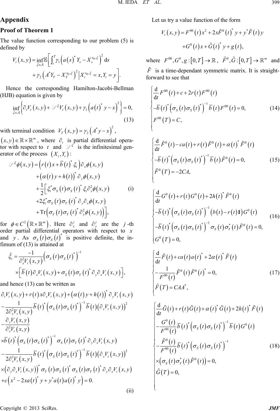 M. IEDA ET AL. 399 Appendix roof of Theorem 1 he value function corresponding to our problem (5) is efined by P T d 0 00 2 *, 1 2 ,, * 2 ,d inf ,. Tx tss t xx TT tt VxyasY Xs YXXxYy Hence the corresponding Hamilton-Jacobi-Bellman JB) equation is given by 0, (13) (H 2 * 1 ,, inf tt t VxyVxyatyx L with terminal condition m 2 * 2 , T Vxy Ayx , ,xy, where t is partial differential opera- tor with respect to t and L is the infinitesimal gen- erator of the process , tt Y: *2 * , 2tS S tx tt xy (i) * * * *2 ,, , 1 2, Tr, , tx y tS Yyx YYy xyrtx btxy ty htxy tt xy tt xy L for . Here * 2m C and are the l operators with respect j-th order partial differentiato and y. As tt * SS is positive ni fim defite, the in- um of (13) is attained at * ,, SS xt xt SYyxt tt btV xyttVxy and hence (13) can be written as 1 * 2 1 ˆ, t Vx y , * 12 ** 2 * 12 2 *** ** 2* ,, 1, 2, , , 2, ,, 20 tt xt SS xt xt xt SS xt xt yxtYSS Yyxt VxyrtxVxytyht btttbtV xy Vxy Vxy t btttbtV xy Vxy Vxyt tt tVx cx xatyyataty . (ii) Let us try a value function of the form where 2 1 ** ** , , 1 xt SS SYyxt Vx y bttttVxy , yt Vxy y * 00 20* * 0 ,2 , t VxyFtxxF t y yFty GtxGtygt 00 0 ,,:0,FGgT, 0,:0, m FG T and is a time-dependant symmetric matrix. It is straight- forward to see that 00 00 1 ** 00 00 d2 d 0, , SS FtcrtFt t btttbtFt FT C (14) * 00 1 ** 0 0 d d 0, 2, SS 0 tcatrtFt tFt t btttbtF t FT CA (15) * 00 0 1 ** 0 1 ** 0 d2 d 0, 0, SS Gt rtGthtFt t btttbtrtGt t GT *0 SS SY bt t tt tF 1 (16) ** * 00 d2 d10, *, 00 tcatat tFt t FtFt Ft FT CAA (17) ** 01 ** 0 00 01 ** 00 *0 d2 d 0, 0, SS SS SY GtrtGtt GthtFt t GtbtttbtG t Ft Ft btt t Ft ttFt GT (18) Copyright © 2013 SciRes. JMF 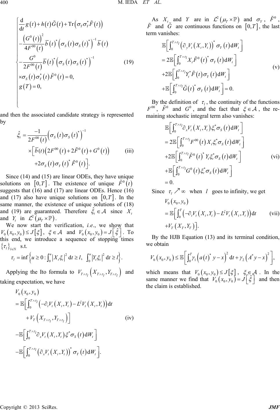 M. IEDA ET AL. 400 * 2 01 ** 00 01 ** 00 *0 dTr d 4 2 0, 0, YY SS SS SY gt htGtFt t Gt bttt bt Ft Gbtt t Ft ttFt gT (19) and then the associated candidate strategy is represented by 1 * 00 0000 *0 1 ˆ2 () 22 2. tSS SY tt Ft btFtFtG t ttFt (iii) Since (14) and (15) are linear ODEs, they have solutions on unique 0,T. The existence of unique 0 t nce (16) suggests that (1d (17) are linear ODEs. He and (17) alsonique solutions on 6) an have u 0,T utions si . In the of (18) nce t same maexistence of unique sol and (19) arenteed. Therefore nner, the guaraˆt ow that and in the verification, t Y We . now start 2T i.e., we sh 000 ,Vxy J , and 000 ˆ ,Vxy J nce of stopping tim . To quees this end, we ll s.t. introduce a se 22 uu 00 inf0:d, d. lt ttt uXtlYtl Applying the Ito formula tol taking expectation, we have d , TTT ll VXY and 000 0 * 0 * 0 , ,, , ,d ,d. Tlttt ttt t TlxtttSt TlxtttYt Vxy VXY LVXYt VXY VXYt W VXYt W TT T ll (iv) As t and Y are in 2T and Y , 0 , and G are continuous functions on 0,T, the last term vanishes: * 0, Tl 0 0 * 0 * 0 2 d d0 . d 2 * d ttt Yt TltYt tYt TlYt VXYt W XF tW YFttW GttW Tl t (v) By the definition of l , the continuity of the functions 00 , 0 and 0 G, and the fact that so vanishes: , the re- almaining stochastic integral term * 0 00 * 0 * 0* 0 0* 0 ,d 2d 2d d 0. Tlxtt tt St Tltt St Tltt St TltSt VXYt W tXt W FtYtW Gt tW (vi) e Sincl when l goity, wet es to infin ge 00 , T Vxy 0 0,, ,. tt t tttt TTT VXY LVXYt VXY d (vii) By the HJB Equation (13) and its term we obtain inal condition, 22 ** 000 12 0 ,d T Vxyatyx tAyx , which means that 000 ,Vxy J , . In the me manner we find that 000 ˆ ,Vxy J sa and then the claim is established. Copyright © 2013 SciRes. JMF
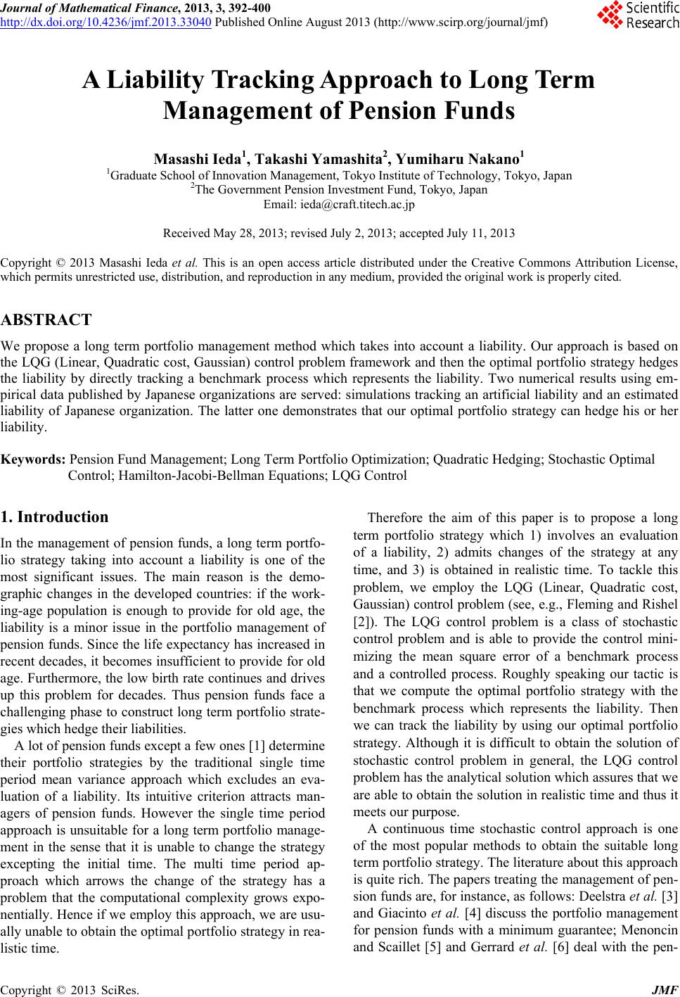
|