American Journal of Computational Mathematics, 2013, 3, 222-230
http://dx.doi.org/10.4236/ajcm.2013.33032 Published Online September 2013 (http://www.scirp.org/journal/ajcm)
Bifurcations and Sequences of Elements in
Non-Smooth Systems Cycles
Ivan Arango1, Fabio Pineda1, Oscar Ruiz2
1Mechatronics and Machine Design Group, Universidad EAFIT, Medellin, Colombia
2Laboratorio de CAD/CAM/CAE, Universidad EAFIT, Medellin, Colombia
Received May 24, 2013; revised July 1, 2013; accepted July 12, 2013
Copyright © 2013 Ivan Arango et al. This is an open access article distributed under the Creative Commons Attribution License,
which permits unrestricted use, distribution, and reproduction in any medium, provided the original work is properly cited.
ABSTRACT
This article describes the implementation of a novel method for detection and continuation of bifurcations in non-
smooth complex dynamic systems. The method is an alternative to existing ones for the follow-up of associated phe-
nomena, precisely in the circumstances in which the traditional ones have limitations (simultaneous impact, Filippov
and first derivative discontinuities and multiple discontinuous boundaries). The topology of cycles in non-smooth sys-
tems is determined by a group of ordered segments and points of different regions and their boundaries. In this article,
we compare the limit cycles of non-smooth systems against the sequences of elements, in order to find patterns. To
achieve this goal, a method was used, which characterizes and records the elements comprising the cycles in the order
that they appear during the integration process. The characterization discriminates: a) types of points and segments; b)
direction of sliding segments; and c) regions or discontinuity boundaries to which each element belongs. When a
change takes place in the value of a parameter of a system, our comparison method is an alternative to determine topo-
logical changes and hence bifurcations and associated phenomena. This comparison has been tested in systems with
discontinuities of three types: 1) impact; 2) Filippov and 3) first derivative discontinuities. By coding well-known cy-
cles as sequences of elements, an initial comparison database was built. Our comparison method offers a convenient ap-
proach for large systems with more than two regions and more than two sliding segments.
Keywords: Bifurcation Sequences; Non-Smooth Systems; Limit Cycles; Dynamic Systems
1. Introduction
Physical systems can often operate in different modes,
and as the time of the transition from one mode to an-
other mode is small, the transition is considered as in-
stantaneous [1]. Events such as impact, dry friction, back-
lash, hysteresis, saturation and commutation carry a dis-
continuity or sudden change. Therefore, they can be mod-
eled declaring at least two modes. Each mode is repre-
sented by differential equation or mixes of differential
and difference equations. The mathematical modeling of
these systems switches between different modes and they
are classified as piecewise-smooth or non-smooth system.
Piecewise-smooth systems may be classified according
to the degree of discontinuity that the orbits and vector
fields present [1]. An updated classification by [2] dis-
cusses systems with three degrees of smoothness. In the
zero level, one has jumps in the state variables. They are
typically systems with impact, where the phenomenon is
modeled assuming no deformation and a negligible im-
pact time [3]. In the first degree of smoothness, we have
systems described by differential equations with discon-
tinuous right hand terms (Filippov systems) [4]. In these
cases the vector field is discontinuous in the switching
Boundary, as usual in mechanical systems with dry fric-
tion [5]. The second degree of smoothness, includes sys-
tems with continuous vector fields but discontinuities in
the first derivative of the vector field. As an example for
second degree, we might consider a mechanical system
with a single mass, spring, damping element and limiting
elastic support [6]. In general, a discontinuity in the i-th
derivative implies that the system is classified as being i
+ 1 degree of smoothness.
Non-standard bifurcations in non-smooth systems have
been intensively studied [6-9]. But, there are only mathe-
matical tools to analyze phenomena in 2D or 3D systems
with two vector fields and one discontinuity boundary
[10,11]. The names assigned to the bifurcations vary ac-
cording to the researcher. For example, [2] is used Graz-
ing, Switching, Crossing and Multisliding. For the same
C
opyright © 2013 SciRes. AJCM

I. ARANGO ET AL. 223
bifurcations, in [12] is used Touching, Bucking, Crossing
and Adding. Other sliding bifurcation types, recently re-
ported in [8], have been characterized in systems with
two DBs. Those bifurcations have been called Exchang-
ing, Sticking Disappearance and Non-smooth Fold.
Article Outline. This article is organized as follows.
Section 2 explains the notation and symbols used. Sec-
tion 3 summarizes the solutions for the types of non-smooth
systems. Section 4 describes the well-known bifurcations
as sequences of elements. Section 5 analyzes the proce-
dure of identification and comparison of the elements of
the cycles versus the elements of an integration. Section
6 concludes the article.
2. Notation and Symbology for Points in the
DB
The study of Non-smooth systems includes more infor-
mation than a smooth system. The proposed method is
based on the information of each element of the cycle.
Therefore, we had to introduce a notation to see all the
information of the points, segments and orbits. The in-
formation should be fully contained inside the textual or
graphical symbols assigned to each element. Some distin-
guished symbols follow.
x: State variable vector, with
()
12
,,,
n
x
xx x=.
Zi: -th smooth region of the space state. i
α: Parameter of the physical system .
()
α ∈
()
,
i
α Fx : Vector field on region i
Z
.
DB: Discontinuity Boundary.
Σij: Discontinuity Boundary between regions i
Z
and
j
Z
.
()
{
}
:,
n
ij ijij
ZZ xH α Σ== ∈=x0
:
:
.
()
,
ij
α x
(
,
ij
H α
xx
H Smooth scalar function defining the
between regions and . .
DB
ij
()
1
,:
nn
ij
H α
+→x
),(
)
Gradient of
α
xHij.
() () ()
1
,,HH αα ∂∂xx
,,,
ij ij
ij
n
Hxx α

=

∂∂

xx.
:
I
i
−
Ω -th component of i
x
before impact.
:
I
i
+
Ω -th component of i
x
after impact.
γ: Impact restitution coefficient
I
I
γ
−+
=Ω Ω

.
:
i
x
G
Point at the end of -th integration step. i
()
,
ij
α x
i
: Vector field that acts on the DB between
regions and , for sliding. j
Cycle equations include indicators, separators and ele-
ments (for cycles: points or segments). Cycles are identi-
fied with a letter C accompanied by a subscript number
(e.g. 4: 4-th cycle). If the cycle contains sliding seg-
ments they appear as superscript preceding the C
letter (e.g. 5: cycle 5 has sliding segments). In the
equations, the symbol Φ is used to represent a com-
posed segment, determined by a sequence of points of a
common type (e.g. 5: a composed segment in region
5). The points are identified with the letter with
super-indices (− or +) indicating whether the point is an
C
S
SC
Φ
Ω
initial (−) or endpoint (+) of a sliding segment S. The
symbol/notes a separator between consecutive elements.
The indicator shows that the elements of the equa-
tion in an evolution are continuously repeated (e.g. :
segment i in region is continuously repeated).
Equations that describe the elements of Bifurcations (cy-
cles) are identified by the symbol
Ò
Ò
i
Φ∕
Φi
β
. Sliding bifurca-
tions are identified with a super-script that precedes
the
S
β
symbol and an alphabetic sub-script that indi-
cates the bifurcation type (e.g. S
c
β
is a sliding crossing
bifurcation).
3. Background of the Non-Smooth Solution
Typically, Non-smooth systems are modeled as piece-
wise-smooth systems (PWS) where the state space
contains four kinds of spaces: Smooth Zones, undefined
Zones associated to regions behind of impact boundaries,
Di s co ntin uity Boundaries with dynamics represented by
convex combinations of the solution of the ODEs of each
vector field and Impact boundaries with dynamic repre-
sented by algebraic equations. Equation (1) shows the
state-space representation of the simplest non-smooth
system with the three types of dynamics.
() ()
{
}
()
{}
() ()
{}
()
()
()
{}
1
1
,,
,if :,0
,if :(,)0
,if :,0
,if :,
n
ii
n
jj
n
ij
n
I
ijk
ZH
ZH
H
H
αα
αα
αα
αα
−
−
∈=∈ >

∈=∈<

=∈Σ =∈=


∈Σ= ∈=







Fx xxx
Fx xxx
xGxx xx
Ixxxx 0
(1)
In Equation (1), i
F
and
j
F are smooth vector fields;
i
Z
and
j
Z
are the corresponding regions and
is a parameter. The state space regions are determined by
the smooth scalar function and the boundary
of impact of
1
α ∈
(
, α x
)
H
i
Z
or
j
Z
regions is determined by the
scalar function .
()
α ,x
I
H
3.1. Zero Degree of Smoothness Systems
In electro-mechanical Non-smooth systems the impact phe-
nomena is highly dynamical, then can be declared using
an algebraic relation due to the impact time is negligible
in relation with the time constant of mechanical systems.
In this relation,
γ
is the restitution coefficient and
()
I
−
Ω
,
()
I
+
Ω
 are respectively the approximation and bounce
speed.
()
() ()
() ()
,II
I
I
I α
γ
+−
+
Ω=Ω

=Ω=Ω


x
−
(2)
The first row of Equation (2) expresses that the posi-
tion before and after the impact are identical. The second
one expresses that the rebound velocity (+) equals the

I. ARANGO ET AL.
224
impact velocity (−) multiplied by the restitution coeffi-
cient
γ
.
3.2. First Degree of Smoothness Systems
Filippov systems, a set of first-order ordinary differential
equations with a discontinuous right-hand side are a sub-
class of discontinuous dynamical systems. The trajectory
of a sliding orbit remaining partially inside the disconti-
nuity boundary may be calculated by the Filippov convex
method as in [4]. Systems with multiple regions and DBs
are treated in [13], where an extended equation for
Filippov systems is described in order to deal with the
intersection of several discontinuity surfaces.
In Filippov systems, between i
Z
and
j
Z
in the dis-
continuity boundary, we assume that there is a region
ij , which are a vector field of dimension con-
formed by three types of points: crossing C, sliding
and singular
(
, and each one with subtypes.
The scalar function is used to determine the
point type, according to the geometric condition of the
vectors in the point of analysis. Equation (3) de-
scribes the geometric conditions of an sliding point.
Equation (4) helps to determine which is the nature of the
point, according to the value of and the neighbor-
ing vector fields at .
Σ
(
S
Ω
1n−
)

(
σ x
(
Ω
)
) )
SO
Ω
(
σ x
x
)
x
()()( )()( )
{
}
,,, ,
xix j
HF HF σα =xxxxx α (3)
()
() () () ()()
()
()
,:
0
0, 0
0
ij
C
SOx ji
S
HF F
σ
σ
σ
∈Σ
Ω>

Ω=∧− =

Ω<


x
x
xxxx
x
)
)
(4)
Crossing points
(
C, characterized by ,
are points which the evolution of the trajectory will not
remain in the . Instead, it crosses from the region in
which has been previously evolving to the other.
Ω
()
0 σ >x
DB
Singular sliding points , characterized by σ (x)
= 0, are points having the associated vectors with the
normal component
(
SO
Ω
()
,
x
i
H
Fx equal to 0. This is
because the vectors are tangential to the DB or vanishes.
At such points: a) i and F
j
F are tangent to the DB; b)
either i or F
j
F
F vanishes while the other is tangent to
the DB; or c) i and
j
F vanish. To avoid the lack of
definition of the Filippov solution for these points, in the
examples, we adopt the methods presented in [14] which
coincide with the topology of the normal forms VV, VI
and II presented in [12].
Sliding points are characterized by .
When a sliding motion is presented in the discontinuity
boundary, the Filippov method gives as a solution a tan-
gent vector to the DB which is a convex combination
, of the vector fields and
(
S
Ω
,ij
∈Σx (Equation (5)).
()()( )(
,,1
i
GF F αλ αλα =+−xx x
)
,
j
(5)
() ()
()()()
,,
,, ,
xj
xji
HF
HF F
α
λαα =−
xx
xx x
(6)
λ
is a scalar function defined through the projections of
the vector fields in the direction of the normal vector
to the discontinuity boundary. According to
the direction of the normal components of the vectors,
the sliding points are stable (or attractor) , or
unstable (or repulsive) (Equation (7)).
() (
xx
)
)
)
H
(
SS
Ω
(
SU
Ω
()
()
()
()
()
()
()
()
,
,0 ,
:,0 ,
SSx ixj
ij
SUx ixj
HH
x
HH
Ω>∧ <

∈Σ 
Ω<∧ >


xF xF
xFxF
0
0
(7)
From Equation (4) the crossing set is open but the
sliding set is closed, it is the union of the sliding seg-
ments, singular points and isolated or special sliding
points. In this paper, the terms special points or isolated
points refer to points whose neighbor points belong to a
different class.
Special points define important dynamics in the sliding
segments of 2d systems or areas in 3D systems. These
points are: a) Equilibria points, in which both vectors i
F
and
j
F
are attractive, transversal to the and are at
the end of two sliding segments pointing each other. b)
Quasi-equilibria points with both vectors i and
DB
F
j
F
attractive transversal or anti collinear and which are at
the start of two sliding segments pointing away each
other. The contrary case have also quasi equilibria points:
repulsive, transversal points which are at the end of two
sliding segments pointing each other. c) Boundary equi-
libria points, in which one of the vector i
F
or
j
F
vanishes. d) Tangent points, in which one of the vectors
i
F
or
j
F
is tangent to the DB. [15] is done a more
strict classification giving the characterization of 42
types of points with the objective of differentiate topo-
logies in order to detect bifurcations.
3.3. Second Degree of Smoothness Systems
The second degree of smoothness systems are represent-
ed as variable structure systems having different dynam-
ics in each zone or region. The dynamics of the system
does not allow sliding or stops on the boundary zone, all
points are crossing and hence, there is not a particular
dynamics defined in the limit zone, instead there is a
change of the region equations set.
)
)
()
0 σ <x
(
,G α xi F
j
F at a point
4. Sequences of Well Known Bifurcations
In this and the following sections, we will present the

I. ARANGO ET AL.
225
)
()
(
123
ss
GCC C
β

=
)
s
(11)
cycles of the most referenced sliding bifurcations as se-
quences of elements. In each cycle are presented the con-
stituent elements assuming that its presence was detected,
in the same order, in the evolution of a dynamical system.
In next equations the symbol is used to represent
segments composed by the same type of point. Arrows
indicate the direction of the sliding segments related to
the DB.
Φ
Impact systems also present grazing bifurcations. An
orbit that is evolving in a region, due to a change in a
parameter, makes contact with a boundary in only one
point. This point has approximation speed equal to zero.
Consequently, the bouncing speed is also zero. If the
physical parameter continues changing, the approxima-
tion and rebound points separate. The corresponding cy-
cles are:
4.1. Grazing Bifurcation
The Grazing Bifurcation
(
s
G
β
occurs in the following
sequence of changes. First, there is an orbit of a limit
cycle 1 evolving in only one of the regions or ,
without hitting the boundary, as shown in Figure 1(a).
Ci j
()
() ()
1
2
3
Ò
Ò
Ò
i
i
iI
i
iI I
C
C
C
+−
+−
=Φ
=Φ Ω
=Φ ΩΩ
(12)
1Ò i
C=Φ (8) 4.2. Switching Bifurcation
Then, when the parameter changes, for example,
from 1 to 2, the cycle grows or moves toward the
discontinuity and has a tangent contact with the last point
of a sliding segment
α
α α
()
s
+
Ω. The structure presented cor-
responds to a type cycle.
2
sC
The sequence of changes for a Switching Bifurcation
(
s
S
)
β
is as follows: the sliding piece of a limit cycle of
type 3 grows until it reaches the first point of
the sliding segment. See Figure 1(d). The type of struc-
ture presented, corresponds to a cycle 4. In general,
the second cycle always characterizes the bifurcation
type and it is only presented for one value of the para-
meter or a very narrow range in the numerical calculation
terms.
SC
()
S
−
Ω
sC
()
2Ò
s
is
C+ =Φ Ω (9)
Subsequently, as the parameter is moved further, the
limit cycle changes again as is depicted in Figure 1(c).
The structure presented corresponds to a type cycle.
3
sC
() ()
4Ò
s
iss s
C−
→
=Φ ΩΦΩ
()
3Ò
s
is s
C+
→
=Φ ΦΩ (10) +
(13)
With a further change in the parameter, the orbit has
now three segments: two of them, i and Φ
j
Φ are in
two different regions separated by the discontinuity bound-
ary, and the third piece is on the sliding region moving to
the right. See Figure 1(e). The structure presented cor-
responds to a type cycle.
5
sC
The orbit of the limit cycle 3 has now two differ-
ent pieces: one without touching the discontinuity bound-
ary and the other one, corresponding to a sliding segment
sC
s
→
Φ that starts in any intermediate point of the discon-
tinuity and ends at a tangent point
()
s
+
Ω. The equation
describing the sequence of cycles is:
Figure 1. Grazing (a)-(c), Switching (c)-(e) and Crossing (e)-(g) bifurcations.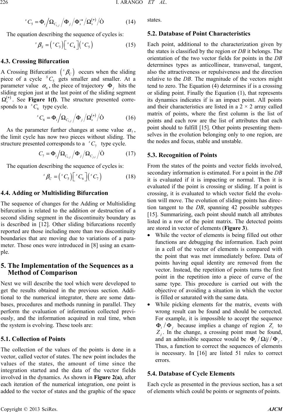

I. ARANGO ET AL.
226
()
,
5Ò
ij
s
iCj ss
C+
→
=Φ ΩΦΦΩ (14)
The equation describing the sequence of cycles is:
()(
345
ssss
SCCC
β

=
)
)
(15)
4.3. Crossing Bifurcation
A Crossing Bifurcation
(
s
C
β
occurs when the sliding
piece of a cycle 5 gets smaller and smaller. At a
parameter value 6, the piece of trajectory
SC
α
j
Φ hits the
sliding region just at the last point of the sliding segment
()
s
+
Ω. See Figure 1(f). The structure presented corre-
sponds to a type cycle.
6
sC
()
,
6Ò
ij
s
iC js
C+ =Φ ΩΦΩ (16)
As the parameter further changes at some value 7,
the limit cycle has now two pieces without sliding. The
structure presented corresponds to a type cycle.
α
7
sC
,,
7Ò
ij ji
iC jC
C=Φ ΩΦΩ (17)
The equation describing the sequence of cycles is:
() (
567
ssss
CCCC
β

=
)
(18)
4.4. Adding or Multisliding Bifurcation
The sequence of changes for the Adding or Multisliding
bifurcation is related to the addition or destruction of a
second sliding segment in the discontinuity boundary as
is described in [12]. Other sliding bifurcations recently
reported are those including more than two discontinuity
boundaries that are moving due to variations of a para-
meter. Those ones were introduced in [8] using an exam-
ple.
5. The Implementation of the Sequences as a
Method of Comparison
Next we will describe the tool which were developed to
get the results obtained in the previous section. Addi-
tional to the numerical integrator, there are some data-
bases, procedures and methods running in parallel. They
perform the evaluation of information collected previ-
ously, and the information acquired in real time, when
the system is evolving. These tools are:
5.1. Collection of Points
The collection of the values of the points is done in a
vector, called vector of states. The new point includes the
values of the states, the amount of time since the
integration started and the data of the vector fields
involved in the dynamics. As shown in Figure 2(a), after
each iteration of the numerical integration, one point is
added to the vector of states and the graphic of the space
states.
5.2. Database of Point Characteristics
Each point, additional to the characterization given by
the states is classified by the region or DB it belongs. The
orientation of the two vector fields for points in the DB
determines types as anticollinear, transversal, tangent,
also the attractiveness or repulsiveness and the direction
relative to the DB. The magnitude of the vectors might
tend to zero. The Equation (4) determines if is a crossing
or sliding point. Finally the Equation (1), that represents
its dynamics indicates if is an impact point. All points
and their characteristics are listed in a 2 × 2 array called
matrix of points, where the first column is the list of
points and each row are the list of attributes that each
point should to fulfill [15]. Other points presenting them-
selves in the evolution belonging only to one region, are
the nodes and focus, stable and unstable.
5.3. Recognition of Points
From the states of the points and vector fields involved,
secondary information is estimated. For a point in the DB
it is evaluated if it is impacting or normal. Then it is
evaluated if the point is crossing or sliding. If a point is
crossing, it is evaluated to which vector field the evolu-
tion will move. The evolution of sliding points has direc-
tion tangent to the DB, spanning 42 possible subtypes
[15]. Summarizing, each point should match all attributes
listed in a row of the point matrix. The detected points
are stored in vector of elements (Figure 3).
• While the vector of elements is being filled out other
functions are debugging the information. Each point
in a cell of the vector of elements is compared with
the point that was met immediately before. Data of
points having equal identity are removed from the
vector. Instead, the repetition of points turns the first
point in the repetition into a piece of curve of the
same type. This procedure is carried out with the
objective of avoiding a situation in which the vector
is filled or saturated with the same data.
• While picking elements for the matrix, events with
wrong result can be found and should be corrected.
For example, it is impossible to accept the sequence
ij
ΦΦ∕ because implies a change of region i
Z
to
j
Z
. In the change, a crossing point must be found,
and an admissible sequence would be ij .
Thus, a function to correct the sequences of elements
is necessary. In [16] are listed 51 rules to correct
errors.
ijΦΩ Φ∕∕
5.4. Database of Cycle Elements
Each cycle as presented in the previous section, has a set
of elements which could be points or segments of points.

I. ARANGO ET AL. 227
Figure 2. Implementation of Cycle Bifurcation. (a) Process of filling the vector with elements appearing in the numeric
integration; (b) Searching process for a specific cycle; (c) Cycle tracking process for bifurcations detection; (d) Cycle
continuation process.
The order of the elements also determines the cycle. In
order to have a wider data base all papers in the literature
should be analyzed and the cycles presented must be
converted in sequences of elements. The information is
stored in a bidimensional array, called matrix of cycles,
in which each row are the identities of the elements of a
cycle.
5.5. Comparison of Cycles
In this step the comparison between the matrix of cycles
and the vector of elements is performed. We wish to
know whether inside the vector of elements there exists a
sub-vector of consecutive and ordered elements that
matches with some row of the matrix of cycles. The se-
quence in the appearance of cycles (and other dynamics)
in this step is recorded in a vector called vector of cycles.
The result in the vector of cycles, for a given set of pa-
rameters, admits the presence of a) equilibrium points, b)
limit cycles, and c) chaotic behavior. For time-varying
parameters, the system evolution might be a sequence
of n cycle types, whose order is dictated by the system
nature (Figures 2(b) and (c)).
To prevent that a repetition of a cycle be mistaken as a
single cycle, a function running in parallel with the inte-
grator performs the evaluation and the correction. When
a sub-sequence of the vector of elements, beginning in
the position 1, is equal to the sub-sequence beginning
in the position 21
nb
j
nbnb l=+ and
j
l is the number of
elements of the cycle, it is concluded that a cycle is
repeating. A cycle is completed when a sequence of
elements is continuously repeated and the time
Γ
to
repeat becomes constant. Let us assume, as illustration, a
sequence with a grazing cycle s . After some
time , the matrix of elements would contain a cycle
with the sequence , which
is not correct.
()
+
ΦΩ∕
i
ΦΩ∕
()
is
++
∕
3Γ
()
is
ΦΩ∕∕
()
is
ΦΩ∕
+
If the search is for a specific cycle, the procedure is
slightly different. In this case, the number of elements in
the cycle under consideration is a date and then it is
reserved the same amount of cells to store the elements
during the integration process. When a new element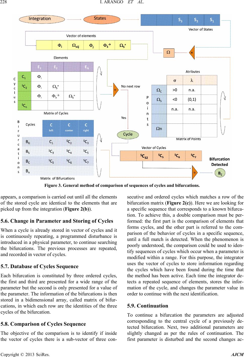

I. ARANGO ET AL.
228
Figure 3. General method of comparison of sequences of cycles and bifurcations.
appears, a comparison is carried out until all the elements
of the stored cycle are identical to the elements that are
picked up from the integration (Figure 2(b) ).
5.6. Change in Parameter and Storing of Cycles
When a cycle is already stored in vector of cycles and it
is continuously repeating, a programmed disturbance is
introduced in a physical parameter, to continue searching
the bifurcations. The previous processes are repeated,
and recorded in vector of cycles.
5.7. Database of Cycles Sequence
Each bifurcation is constituted by three ordered cycles,
the first and third are presented for a wide range of the
parameter but the second is only presented for a value of
the parameter. The information of the bifurcations is then
stored in a bidimensional array, called matrix of bifur-
cations, in which each row are the identities of the three
cycles of the bifurcation.
5.8. Comparison of Cycles Sequence
The objective of the comparison is to identify if inside
the vector of cycles there is a sub-vector of three con-
secutive and ordered cycles which matches a row of the
bifurcation matrix (Figure 2(c)). Here we are looking for
a specific sequence that corresponds to a known bifurca-
tion. To achieve this, a double comparison must be per-
formed: the first part is the comparison of elements that
forms cycles, and the other part is referred to the com-
parison of the behavior of cycles in a specific sequence,
until a full match is detected. When the phenomenon is
poorly understood, the comparison could be used to iden-
tify sequences of cycles which occur when a parameter is
modified within a range. For this purpose, the integrator
uses the vector of cycles to store information regarding
the cycles which have been found during the time that
the method has been active. Each time the integrator de-
tects a repeated sequence of elements, stores the infor-
mation of the cycle, and changes the parameter value in
order to continue with the next identification.
5.9. Continuation
To continue a bifurcation the parameters are adjusted
corresponding to the central cycle of a previously de-
tected bifurcation. Next, two additional parameters are
slightly changed as per the rules of continuation. The
first parameter is disturbed and the second changes ac-

I. ARANGO ET AL. 229
cordingly, to keep the dynamics of the central cycle. This
controlled disturbance of the two parameters is repeated,
such that it determines a trajectory in a continuation-plot.
The change of parameters could be done using methods
like predictor-corrector described in [17] or [18]. In this
cases, the predictive function is the cycle that generates
the bifurcation, and the previous and posterior cycles to
the bifurcation are used for correction.
Figure 2(d) shows an example of how is used the
method of comparison. The first step is a sensibility
analysis that indicates to which cycle, the system evolves
when the parameters are increased or decreased. For
example, the bifurcation 2 has a sequence of cycles
5
. Assume that a direct proportional
sensibility exists for parameter 1. This implies that a
small increment in the parameter value tends to change
the cycle into and a small decrement tends to change
the cycle into 3. Changing 1, the cycle 4 is
obtained. Then, the second parameter 2 is decreased
(in this case the initial point has a high value). After the
change in parameter 2, the cycle 4 changes to
3 or to 5. In the first case, the continuation algo-
rithm increases 1 until the cycle type 4 is found
again. In the second case, the algorithm acts conversely.
The process is continuously iterated until the prescribed
final value of parameter is reached.
SC
α
() (
34
SSS
CCC


5
SC
SC
SCSC
α
)
α
α
SC
α
SC
S
α
C
2
Two objectives of an application for automatic bifur-
cation detection are: 1) to perform the detection task
without a close supervision; and 2) to track bifurcations
through continuation. The procedures developed here can
be used to achieve these goals.
6. Conclusions
This article presents an alternative method for detecting
bifurcations of limit cycles in non-smooth systems. We
focused on complex systems, which defy boundary-value
methods. The comparison method, reported in this article,
is not intended to focus in the same achievements of
other methods. Instead, it addresses open issues left by
them, such as multiple sliding segments and discontinu-
ity boundaries (DB). The comparison method differs
from other approaches in the identification and manipu-
lation of the system information. While the methods in
[10,11] consider a system as one entity to be solved by a
group of equations, the comparison method uses previ-
ously collected information in a data base of points, cy-
cles and bifurcations. This information allows compari-
sons and decision making. To enable the method for
non-smooth systems, the cases when the evolution
crosses the DBs of systems having simultaneously the
three degrees of smoothness (impact, Filippov and first
derivative discontinuities) was analyzed. To achieve the
goal was used the method that characterizes and records
the elements comprising the cycles in the order they ap-
pear in the integration process. The cycles were charac-
terized as sequences of elements (points and segments).
It must be noticed that the sequence of cycles has the
topological changes (e.g. bifurcations) implicit. Some of
the types of data considered as topological characteristic
and collected during the evolution are: a) number of ele-
ments of the cycle; b) order in which the cycle elements
are generated; c) position of the sliding elements in the
sequence of cycle generation; d) way (e.g. extreme or
interior) in which the cycle reaches and leaves the sliding
segment; e) discontinuity boundary to which the element
belongs; f) direction (CW, CCW) in which the cycle
evolves. In this article we also report a textual notation to
describe the elements of the cycles. The comparison
method is also able to handle continuation of sliding
bifurcations.
The method of comparison could be implemented us-
ing tools of the sequence theory, suffix-trees and string-
matching, which offer procedures to drive a large number
of elements and allow us to discriminate subsets with low
computing time investment. The procedure of compari-
son fulfills the two tasks required by an application for
automatic bifurcations detection: perform the detection
task without a closed supervision and track bifurcations
through continuation.
REFERENCES
[1] M. Amorin, S. Divenyi, L. Franca and H. I. Weber, “Nu-
merical and Experimental Investigations of the Nonlinear
Dynamics and Chaos in Non-Smooth Systems,” Journal
of Sound and Vibration, Vol. 301, No. 1-2, 2007, pp. 59-
73. doi:10.1016/j.jsv.2006.09.014
[2] I. Arango, “Singular Point Tracking: A Method for the
Analysis of Sliding Bifurcations in Non-smooth Sys-
tems,” PhD Thesis, Universidad Nacional de Colombia,
2011.
[3] I. Arango and J. A. Taborda, “Integration-Free Analysis
of Non-smooth Local Dynamics in Planar Filippov Sys-
tems,” International Journal of Bifurcation and Chaos,
Vol. 19, No. 3, 2009, pp. 947-975.
doi:10.1142/S0218127409023391
[4] M. Bernardo, C. Budd, A. R. Champneys and P. Kowalc-
zyk, “Piecewise-Smooth Dynamical Systems: Theory and
Applications,” Springer, Berlin, 2008.
doi:10.1007/978-1-84628-708-4
[5] P. Casini and F. Vestroni, “Nonstandard Bifurcations in
Oscillators with Multiple Discontinuity Boundaries,” Non-
linear Dynamics, Vol. 35, No. 1, 2004, pp. 41-59.
doi:10.1023/B:NODY.0000017487.21283.8d
[6] A. Colombo, M. Di Bernardo, E. Fossas and M. R. Jef-
frey, “Teixeira Singularities in 3D Switched Feedback
Control Systems,” Systems & Control Letters, Vol. 59,
No. 10, 2010, pp. 615-622.
doi:10.1016/j.sysconle.2010.07.006

I. ARANGO ET AL.
230
[7] F. Dercole and Y. Kuznetsov, “SlideCont: An Auto97
Driver for Bifurcation Analysis of Filippov Systems,”
ACM Transactions on Mathematical Software (TOMS),
Vol. 31, No. 1, 2005, pp. 95-119.
doi:10.1145/1055531.1055536
[8] L. Dieci and L. Lopez, “Sliding Motion in Filippov Dif-
ferential Systems: Theoretical Results and a Computa-
tional Approach,” SIAM Journal on Numerical Analysis,
Vol. 47, No. 3, 2009, pp. 2023-2051.
doi:10.1137/080724599
[9] A. Filippov and F. Arscott, “Differential Equations with
Discontinuous Righthand Sides: Control Systems, Vol-
ume 18 of Mathematics and Its Applications: Soviet Se-
ries,” Springer, Berlin, 1988.
[10] M. Guardia, T. M. Seara and M. A. Teixeira, “Generic
Bifurcations of Low Codimension of Planar Filippov Sys-
tems,” Journal of Differential Equations, Vol. 250, No. 4,
2011, pp. 1967-2023. doi:10.1016/j.jde.2010.11.016
[11] Y. Kuznetsov, S. Rinaldi and A. Gragnani, “One-Parame-
ter Bifurcations in Planar Filippov Systems,” Interna-
tional Journal of Bifurcation and Chaos, Vol. 13, No. 8,
2003, pp. 2157-2188. doi:10.1142/S0218127403007874
[12] R. I. Leine, “Bifurcations in Discontinuous Mechanical
Systems of Filippov-Type,” PhD Thesis, Technische Uni-
versiteit Eindhoven, 2000.
[13] W. Marszalek and Z. Trzaska, “Singular Hopf Bifurca-
tions in DAE Models of Power Systems,” Energy and
Power Engineering, Vol. 3, No. 1, 2011, pp. 1-8.
doi:10.4236/epe.2011.31001
[14] I. Merillas, “Modeling and Numerical Study of Non-
smooth Dynamical Systems: Applications to Mechanical
and Power,” PhD Thesis, Technical University of Catalo-
nia, 2006.
[15] I. Arango and J. A. Taborda, “Integration-Free Analysis
of Non-Smooth Local Dynamics in Planar Filippov Sys-
tem,” International Journal of Bifurcation and Chaos,
Vol. 19, No. 3, 2009, pp. 947-975.
[16] A. Nordmark, “Existence of Periodic Orbits in Grazing
Bifurcations of Impacting Mechanical Oscillators,” Non-
linearity, Vol. 14, No. 6, 2001, pp. 1517-1542.
doi:10.1088/0951-7715/14/6/306
[17] T. S. Parker and L. Chua, “Practical Numerical Algo-
rithms for Chaotic Systems,” Springer Limited, London,
2011.
[18] P. Thota and H. Dankowicz, “TC-HAT (TC): A Novel
Toolbox for the Continuation of Periodic Trajectories in
Hybrid Dynamical Systems,” SIAM Journal on Applied
Dynamical Systems, Vol. 7, No. 4, 2008, pp. 1283-1322.
doi:10.1137/070703028