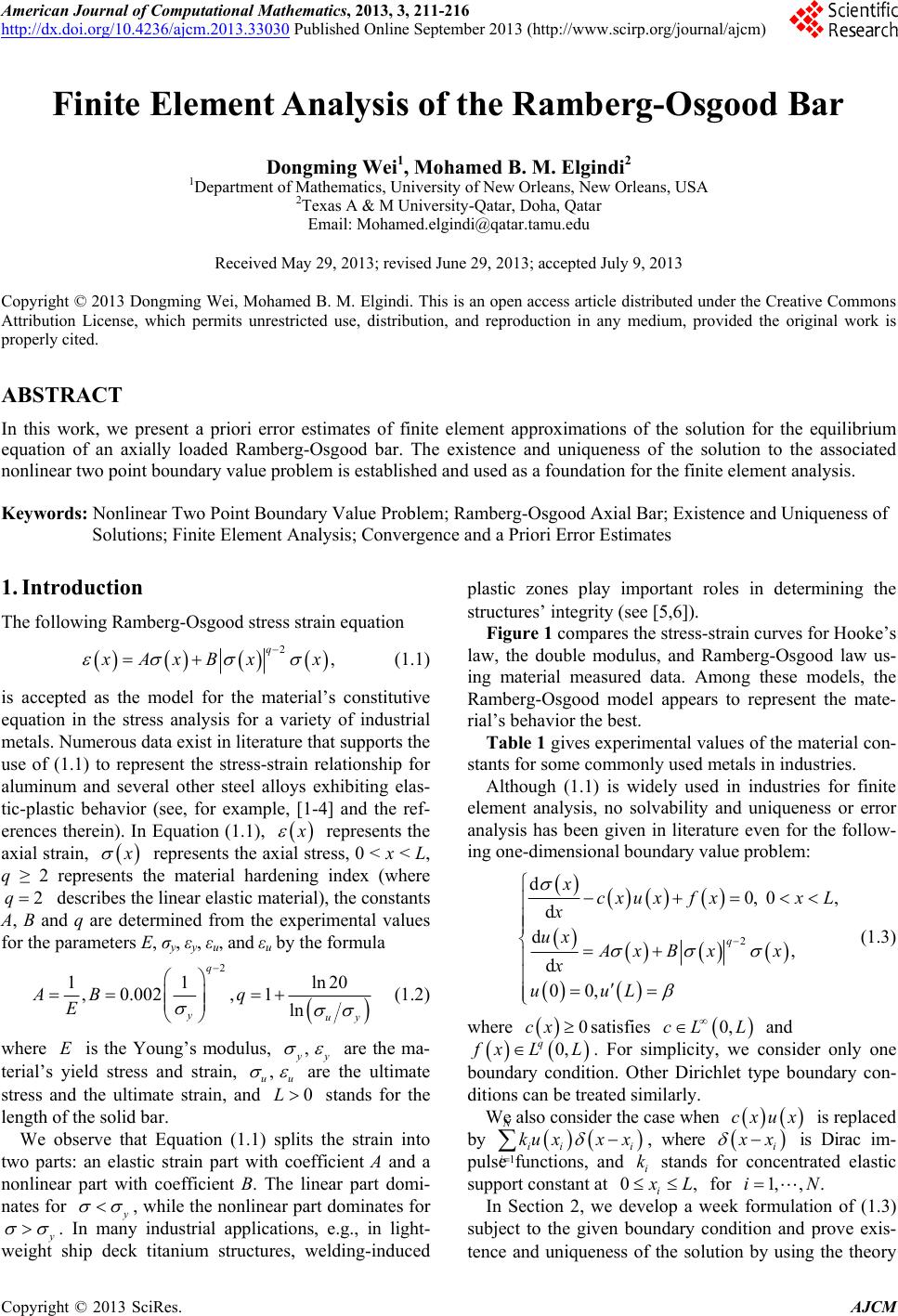
American Journal of Computational Mathematics, 2013, 3, 211-216
http://dx.doi.org/10.4236/ajcm.2013.33030 Published Online September 2013 (http://www.scirp.org/journal/ajcm)
Finite Element Analysis of the Ramberg-Osgood Bar
Dongming Wei1, Mohamed B. M. Elgindi2
1Department of Mathematics, University of New Orleans, New Orleans, USA
2Texas A & M University-Qatar, Doha, Qatar
Received May 29, 2013; revised June 29, 2013; accepted July 9, 2013
Copyright © 2013 Dongming Wei, Mohamed B. M. Elgindi. This is an open access article distributed under the Creative Commons
Attribution License, which permits unrestricted use, distribution, and reproduction in any medium, provided the original work is
properly cited.
ABSTRACT
In this work, we present a priori error estimates of finite element approximations of the solution for the equilibrium
equation of an axially loaded Ramberg-Osgood bar. The existence and uniqueness of the solution to the associated
nonlinear two point boundary value problem is established and used as a foundation for the finite element analysis.
Keywords: Nonlinear Two Point Boundary Value Problem; Ramberg-Osgood Axial Bar; Existence and Uniqueness of
Solutions; Finite Element Analysis; Convergence and a Priori Error Estimates
1. Introduction
The following Ramberg-Osgood stress strain equation
 
2, q
x
Ax Bxx  

 (1.1)
is accepted as the model for the material’s constitutive
equation in the stress analysis for a variety of industrial
metals. Numerous data exist in literature that supports the
use of (1.1) to represent the stress-strain relationship for
aluminum and several other steel alloys exhibiting elas-
tic-plastic behavior (see, for example, [1-4] and the ref-
erences therein). In Equation (1.1),

x
 represents the
axial strain,

x
 represents the axial stress, 0 < x < L,
q ≥ 2 represents the material hardening index (where
describes the linear elastic material), the constants
A, B and q are determined from the experimental values
for the parameters E, σy, εy, εu, and εu by the formula
2q

2
11 ln
,0.002 ,1
ln
q
yuy
AB q
E

20




 



(1.2)
where is the Young’s modulus, E,
y
y


u
are the ma-
terial’s yield stress and strain, ,
u


0L
are the ultimate
stress and the ultimate strain, and stands for the
length of the solid bar.
We observe that Equation (1.1) splits the strain into
two parts: an elastic strain part with coefficient A and a
nonlinear part with coefficient B. The linear part domi-
nates for
y

 , while the nonlinear part dominates for
y

 . In many industrial applications, e.g., in light-
weight ship deck titanium structures, welding-induced
plastic zones play important roles in determining the
structures’ integrity (see [5,6]).
Figure 1 compares the stress-strain curves for Hooke’s
law, the double modulus, and Ramberg-Osgood law us-
ing material measured data. Among these models, the
Ramberg-Osgood model appears to represent the mate-
rial’s behavior the best.
Table 1 gives experimental values of the material con-
stants for some commonly used metals in industries.
Although (1.1) is widely used in industries for finite
element analysis, no solvability and uniqueness or error
analysis has been given in literature even for the follow-
ing one-dimensional boundary value problem:

 
  
 
2
d0, 0,
d
d,
d
00,
q
xcxuxf xxL
x
ux Ax Bxx
x
uuL
















(1.3)
where


0cxsatisfies and

0,cL L







0,
q
L Lfx . For simplicity, we consider only one
boundary condition. Other Dirichlet type boundary con-
ditions can be treated similarly.
We also consider the case when is replaced
by
1i
, where

cxux

i

N
ii i
ku xxx  

x
x   is Dirac im-
pulse functions, and stands for concentrated elastic
support constant at
i
k
0,
i
x
L

 for 1, ,iN.
In Section 2, we develop a week formulation of (1.3)
subject to the given boundary condition and prove exis-
tence and uniqueness of the solution by using the theory
C
opyright © 2013 SciRes. AJCM

D. WEI, M. B. M. ELGINDI
212
0
5
10
15
20
25
30
35
40
45
50
00.01 0.02 0.03 0.04 0.050.060.070.08 0.09
STRESS(ksi)
STRAIN(in/in)
FourdifferentStress/Strainmodels,comparedwithmeasureddata
MeasuredData‐ Material1
MeasuredData‐ Material2
Hooke'sLaw,Material1
Hooke'sLaw,Material2
Ramberg‐Osgood,Material1
Ramberg‐Osgood,Material2
Reduce dModulusModel‐ Material1
Reduce dModulusModel‐ Material2
Figure 1. Ramburg-Osgood curves.
Table 1. Constants for Ramburg-Osgood materials.
Material A B q − 1
Inconel 718 3.33e−05 4.42e−71 32.00
5083 Aluminum 9.80e−05 2.50e−23 13.11
6061T6 Aluminum 1.00e−04 1.35e−58 34.44
304 Stainless Steel 3.57e−05 3.44e−13 6.32
304 L StainlessSteel 3.57e−05 2.24e−15 7.36
of perturbed convex variational problems in Sobolev
spaces (see [7] for details.) We also prove that the solu-
tion is bounded in certain Sobolev norms. In Section 3,
we derive an error estimates for the semi-discrete error
between the week solution and the Galerkin’s finite ele-
ment solution of (1.3) for the standard conformal finite
elements. The results of this section are based on the re-
sults in Section 2. We believe that the results established
in these sections are novel and preliminary.
2. Existence and Uniqueness of Solutions
Let and be the standard Sobo-

1, 0, p
W
lev spaces, where .
1
q
pq 

Define

2q
AB



  , where 0,0, and 2.AB q 

Observe that the mapping

 is one-to-one; how-
ever, its inverse cannot be written explicitly.
Since u



, Equation (1.3) can be rewritten as:
 
 
1
d() , 0
d
, 00,
xcxuxf xxL
x
uu uL

 











(2.2)
Define the following space of admissible functions as
 


1, 0,0 0,. p
VuW LuuL


 (2.3)
The weak formulation of (2.2) can then be written as
Problem I: Find uV

, such that
 
11
0
000
ddd0,
LLl
p
uvxcuvxfvxvWL 
 
,
. (2.4)

L

L

1,
00,
p
WLet us define the operator:

D. WEI, M. B. M. ELGINDI 213
 
1
00
,d
LL
auvuv xcuvx 



d,

(2.5)
for . Then, satisfies the following prop-
erty:
,uv V


,auv



 
 
 
2
00
11
12
2
1 1
2
21 1
00
2
11
,dd
d
dd
,for.
q
LL
q
LL q
q
LL
uu xcux
uAu Buux
cu xAuBux
Au BuuV
  







 

 



  


  


0
L
auu 

(2.6)
Also, by the definition of

, we have
 
 
 
2
111
1
11
1
11
qq
qq
qq
q
L
L
q
LL
q
LL
uAuBuu
AuB u
Au Bu











 
 

(2.7)
Lemma 2.1 For given positive constants ,,,
A
Bq L,
there exists a constant independent of the solutions
of the BVP (1.3) such that
C

ux V
 
2
2
11
q
q
LL
uuC 


 .
Proof: For a solution

ux V

, we can write:
, where
bb
vuuu

1,
00,
p
vW L
LL
V is a fixed function, so that
, and since:

1
00
dduvxcuvxfvx 
 

0
d
L

d
d
b
, we get:
 

12
00
00 0
1
0
,d
dd
+d
LL
LL L
b
L
b
auuuu xcux
f
uxfuxcuu x
uu x






 


 

(2.8)
Also, by (2.6) and (2.8), we have:
 



2
2
11
1
1
12 3,
q
qpq p
p
q
pq
q
LL
b
LLLL
bL
L
LL
Au Bu
fuu fcu
uu
CCu Cu












 
q
b
L
(2.9)
where


12
,,
qq pq
bb
LLLL
CfuC fcu and
3
p
b
L
Cu

.
By the Sobolev inequality, we have (see e.g. [8,9]):
p
q
L
L
uCu

, and therefore:
 
11
12 3.
q
qq
q
L
L
L
BuCCuC u 


 
Also, since by definition of

,
 
 
 
2
111
1
11
1
11
,
qq
qq
qq
q
L
L
q
LL
q
LL
uAuBuu
AuB u
Au Bu

















we have
  
1
11
12 3 qq
qq
1
q
L
LL
uCCuCu 


    (2.10)
where ,1,2,3
i
Ci are positive constants. From (2.10),
we conclude that


1
q
L
u 


is bounded and that there
exists a constant C such that

1
q
L
uC 
, as


ux
varies over the solution set of (1.3) in Therefore, the
result of the lemma is follows.
.V
Theorem 2.1 For a given , q ≥ 2, A > 0
& B > 0, problem (I) has a unique solution .

0,
q
fL L

uU
Proof:
The uniqueness follows from the following argument.
Let and be two solutions of (2.4). Then (since
1
u2 u


0cx ):
 


11
1212
0
0duuuu 


 

L
x,
which leads to:
 




12 12
0
2
12
0
22
112 212
0
2
12
0
0d
d
d
d,
L
L
Lqq
L
x
Ax
Bx
Ax
 




 

 





since


1
11
u 


, and

1
22
u 





22qq
112 212
0, 


which is well-known [10,11].
Therefore, 12



and 12 u, and this establishes
the uniqueness of the solution of (2.4).
u
For existence, we consider the variational formulation
of (2.4) and define the total potential energy by:


2
00 0
12
00
1ddd
2
1dd
2
LL L
LL
Juxcu xfux
uuxcu xfux












 

0
d
L

D. WEI, M. B. M. ELGINDI
214
Let
 
1
1
2
tt 

t , then

J
u can be written as:
 
2
000
1dd
2
LLL
d.
J
uuxcux 






fux
Also we have:
 
11
11
22
tt t
 


 

t
.
Letting


 
2. q
tytAytBytyt 


Then and

1
y 


 
t

2
11.
q
A
yt q By yt


Therefore, we get
 
  
 
1
2
2
11 1
1, and
1
1
21
1.
2
q
q
tyt
Aq By
t
tyt
Aq By
tt t


 





 

 


 




Now the first variation of J can be expressed as:
 

00
1
00
ddd
d
dd
LL
L
0
.
L
J
uvuvcuvx fvx
uvcuvxfvx






  

 




However:



 


 



4
22
2
2
2
22
2
2
2
12
12
211
12
12
211
1
10.
21
q
qq
q
qq
q
q
t
qqByyy
t
Aq ByAqBy
qqBy
Aq ByAqBy
Aqq By
Aq By














 










 













We rewrite the total energy function as
 
12
J
uFuFuFu, where
 
10
1d
2
L
F
uu 

x

, 2
2
0
1d
2
L
F
ucux , and
 
0d
L
F
ufxuxx. Then weak formulation (2.4) is
equivalent to

Min
uV
J
u


1
0, :tF
.
Since , and since
,
is convexVR 
 

0, L2:cL


F
VR

n
u
 
0,
q
L
is weekly sequentially con-
tinuous (since

converges weekly in implies
that converges strongly in .) Also (2.6)
and (2.7) imply the coercivity of
V
 
n
uL

J
u, see, e.g., [9-11 ].
Therefore,


J
u satisfies the conditions of the theorem
of 42.7, pp. 225-226, in [9], and the existence of a weak
solution follows.
We now consider the second case when the term




cxux is replaced by .

ii
x 
 
1
N
i
i
kux x



In this case,
 
i
ux 
2
2
1
1
2
N
i
i
Fu k

 
 and we only
need show that it is weakly sequentially continuous.
Suppose that


n
u converges weekly in V, then for a


0, L
mvu

0
d
L
k
vu x


ki
ux
1, q
vW 

,
 
lid d
kk
kvuxvux



00
LL
vu

xL
vu


i
and . Therefore, since
0
lim d
L
kvu x  
 
00
dd
i
k k
uxx xx
 
,
where

, 0
,
ii
x
xx
vx
x
xxL



00
d
LL
i
xx
ux




2
ii
u x
x


 


ux



We have

ki
ux
2
lim Fu


x x  
 

0
lim limd
d
i
k
kk
x
vu vuxx
ux x
  
 

 

2
1
2
1
lim
.
N
kiki
kk
i
N
i
k
ku Fu
 



Therefore, Theorem 2.1 holds with the same condi-
tions for the case when is replaced by
cx
 
1
N
iii
i
ku x

.
3. Finite Element Error Estimates
Let




1, 0, q
VS LWL
k
0,
k
hh be a standard conformal
finite element space of order (See [12-15]) satisfying
the interpolation property:


1, 0,,
kp
hp
vv CvhL 1, ,vW (3.1)
where is a positive constant depending only on
and , h
Cv
Lv

is the finite element interpolation of ,
is the polynomial degree for the interpolation shape
functions, and h the mesh size,
v
k
1,
h
p
vv the W1,p(0,
L) norm.
The corresponding finite element Galerkin’s finite
element approximation problem for (2.1) is:

D. WEI, M. B. M. ELGINDI 215
Problem II:
Find
 

0,0 ,,
k
hhhhhh
uVSLvAvL B


such that

1
000
dd
LLL
hhhhhh
uvx uvdxvxfvx 
 


d, (3.2)
 

00,00,0
k
hhhhh
vVvSLvvL

 .
Theorem 3.1 Problem II has a unique solution.
Proof: The proof is similar to the proof of Theorem
2.1.
Lemma 3.1
For given positive constants ,,,
A
Bq L , there exists a
constant independent of the solutions Ch uV
h

of
Problem II such that

1
q
uC
hL

.
Proof:
The proof is similar to that of Lemma 2.1.
To derive finite element error estimates, let de-
notes the exact solution of Problem I and the finite
element solution of Problem II.
u
h
u
Then
 
 




 
 

11
0
0
11
,,
,,
d
d
p
q
p
q
hhh
hhh
L
hh
L
hh
hh
L
L
hh
L
L
auuu auuu
auuuau uu
uuuu
cu uuux
uuuu
cu uuu




 


 
 

 
 


x
(3.3)
Let and . Also

1,u




1,u



 
 

 
    





2
11
00
2
00
22 2
00
2
0
2 2
00
,,
dd
dd
d
d
dd.
hhh
LL
hh h
LL
hhh
LL
q q
hhh
L
h
LL
hh
auuuauu u
uuuuxcuux
xcuux
d
h
A
xB x
cu ux
Axcuux

 



 
 

 

 

 





(3.4)
As a result of (3.3) and (3.4), we get:

  

2
2
22
11
1
q
p
p
q
hh
L
L
hh
L
L
hh
L
L
cu u
uuuu
A
cu uuu






 



 

(3.5)
By Lemma 2.1, Lemma 3.1, and (3.4), we get the
following error estimates:


2
2
22
p
hh
L
L
hh
L
k
cu u
Cuuu u
Ch
 



p
L
0,k
(3.6)
Therefore, by (3.6), we have established the following
convergence and error estimate result.
Theorem 2.3 For
1i
i or
any
 
,
N
ii
cxkx x  



0cx, let and h u be the unique solutions of
Problems I and II, respectively, then
u
2
2k
hLCh
 , and 0 lim 0
p
hL
huu 
 ,
and if


0
cx c
N
for some , or
00c


1
,0
iii
i
cxkx xk 

,


 then
22
22k
hh
LL
uu Ch   , and 1,
0
lim 0
hp
huu


,
in which


1u



 and stand for the
stresses.

1
h
u 

h
Note that

stands for the stress corresponding to
the strain u



.
4. Conclusion
In this work, we establish existence and uniqueness of
the solution of (2.4) in the Sobolev space and its
finite element solution h in a general finite element
space
uU
u


0 with elastic support for a class of load
functions f. We derive convergence and error estimates
for the semi-discrete error .
0,
h
SL
 
hh
exux u

x
5. Acknowledgements
The research in this paper is a part of a research project
funded by the Research office, Texas A & M University
at Qatar.
REFERENCES
[1] W. R. Osgood and W. Ramberg, “Description of Stress-
Strain Curves by Three Parameters,” NACA Technical
Note 902, National Bureau of Standards, Washington DC,
1943.
[2] L. A. James, “Ramberg-Osgood Strain-Harding Charac-

D. WEI, M. B. M. ELGINDI
216
terization of an ASTM A302-B Steel,” Journal of Pres-
sure Vessel Technology, Vol. 117, No. 4, 1995, pp. 341-
345. doi:10.1115/1.2842133
[3] K. J. R. Rasmussen, “Full-Range Stress-Strain Curves for
Stainless Steel Alloys,” Research Report R811, Univer-
sity of Sydney, Department of Civil Engineering, 2001.
[4] V. N. Shlyannikov, “Elastic-Plastic Mixed-Mode Fracture
Criteria and Parameters, Lecture Notes Applied Mechan-
ics, Vol. 7,” Springer, Berlin, 2002.
[5] P. Dong and L. DeCan, “Computational Assessment of
Build Strategies for a Titanium Mid-Ship Section,” 11th
International Conference on Fast Sea Transportation,
FAST, Honolulu, 26-29 September 2011, pp. 540-546.
[6] P. Dong, “Computational Weld Modeling: A Enabler for
Solving Complex Problems with Simple Solutions, Key-
note Lecture,” Proceedings of the 5th IIW International
Congress, Sydney, 7-9 March 2007, pp. 79-84.
[7] E. Zeidler, “Nonlinear Functional Analysis and Its Ap-
plications, Variational Methods and Optimization, Vol.
III,” Springer Verlag, New York, 1986.
doi:10.1007/978-1-4612-4838-5
[8] R. A. Adams, “Sobolev Spaces, Pure and Applied Mathe-
matics, Vol. 65,” Academic Press, Inc., New York, San
Francisco, London, 1975.
[9] V. G. Maz’Ja, “Sobolev Spaces,” Springer-Verlag, New
York, 1985.
[10] F. E. Browder, “Variational Methods for Non-Linear
Elliptic Eigenvalue Problems,” Bulletin of the American
Mathematical Society, Vol. 71, 1965, pp. 176-183.
doi:10.1090/S0002-9904-1965-11275-7
[11] R. Temam, “Mathematical Problems in Plasticity,” Gau-
thier-Villars, Paris, 1985.
[12] G. Strang and G. J. Fix, “An Analysis of the Finite Ele-
ment Method,” Prentice-Hall, Inc., Englewood Cliffs,
1973.
[13] P. G. Ciarlet, “The Finite Element Method for Elliptic
Problems,” North- Holland, Amsterdam, 1978.
[14] J. T. Oden And G. F. Carey, “Finite Elements,” Pren-
tice-Hall, Englewood Cliffs, 1984.
[15] S. C. Brenner and L. R. Scott, “The Mathematical Theory
of Finite Element Methods, Texts in Applied Mathemat-
ics, v. 15,” 3rd Edition, Springer Verlag, New York, 2008.
doi:10.1007/978-0-387-75934-0