Paper Menu >>
Journal Menu >>
 J. Serv. Sci. & Management. 2008, 1: 11-20 Published Online June 2008 in SciRes (www.SRPublishing.org/journal/jssm) Copyright © 2008 SciRes JSSM Extended TOPSISs for Belief Group Decision Making Chao Fu School of Management, Hefei University of Technology, Hefei 230009, China ABSTRACT Multiple attribute decision analysis (MADA) problems in the situation of belief group decision making (BGDM) are a special class of decision problems, where the attribute evaluations of each decision maker (DM) are represented by belief functions. In order to solve these special problems, in this paper, TOPSIS (technique for order preference by similarity to ideal solution) model is extended by three approaches, by which group preferences are aggregated in dif- ferent manners. Corresponding to the three approaches, three extended TOPSIS models, the pre-model, post-model, and inter-model, are developed and their procedures are elaborated step by step. Aggregating group preferences in the three extended models respectively depends on Dempster’s rule or its modifications, some social choice functions, and some mean approaches. Furthermore, a numerical example clearly illustrates the procedures of the three extended models for BGDM. Keywords: basic belief assignment, belief group decision making, belief preferences aggregation, TOPSIS 1. Introduction Recently, the uncertain multiple attribute decision analy- sis (MADA) problems with a group of decision makers (DMs) have been widely studied in the literature, in which the attribute evaluations are unknown, vague, partial known, or imprecise. The representative solution is to construct a fuzzy TOPSIS (technique for order preference by similarity to ideal solution), a classical modified ap- proach for uncertain MADA problems, to choose the best one from a set of alternatives [2-4, 18, 20, 30]. However, compared with the Dempster-Shafer theory (DST) [5,23], the operators of fuzzy set theory (FST) to aggregate group preferences, which are usually the ar- ithmetical mean, the geometric mean, or their modifica- tions, are less adaptable and available. Hence, this paper uses the DST to describe uncertain MADA problems; that is to say, it uses basic belief assignments (bbas) to repre- sent uncertain attribute evaluations. In practice, due to the one-to-one correspondence be- tween the bba and the belief function [23], the bba is usually either elicited from experts, or constructed from observation data. To transform qualitative experts’ opin- ions into bbas, some methods have been proposed by Wong and Lingras [31], Bryson and Mobolurin [1], and Yaghlane et al. [34]. Using the bba to represent uncertain group attribute evaluations, one correspondingly converts the group decision making (GDM) to the belief group decision making (BGDM). To solve MADA problems in the situation of BGDM, the original TOPSIS [15] is extended by three approaches described in [25]. Their operators to aggregate group preferences are respectively the pre-operation, post-opera- tion, and inter-operation. Based on Yang’s rule and utility based equivalent transformation of the assessments on different frames of discernment [35], the evaluations on different attributes related to different frames can be unified to become the ones on a common frame. Furthermore, the positive and negative preference vectors of DM, the positive ideal solution of belief (PISB), and the negative ideal solution of belief (NISB) are constructed. The preference vectors avoid the possible paradoxes between the calculating ranks of alternatives and the fact of DM’s preference, and the PISB and NISB are used to determine the ranks of alternatives. The detailed extended models are explained step by step in Section 3. The rest of this paper is organized as follows. In Section 2, the related foundations are reviewed. Section 3 dis- cusses three extended models in accord with three ap- proaches to aggregating group preferences, the pre-operation, post-operation, and inter-operation, in or- der to make solutions to BGDM. A numerical example is given in Section 4 to illustrate the procedures of three extended models and their differences. At last, Section 5 concludes this paper. 2. Review of Related Foundations 2.1. Basics of bba In a specific application domain, the DST first defines Ω, called the frame of discernment, containing N exhaustive and exclusive hypotheses. Let 2Ω denote the power set composed of 2N propositions of A such that A⊆Ω. Definition 1. Let Ω denote a frame of discernment, and S be a piece of arbitrary evidence source (ES) on Ω. Thus, the bba of ES is defined by m: 2Ω→ [0, 1]. This function 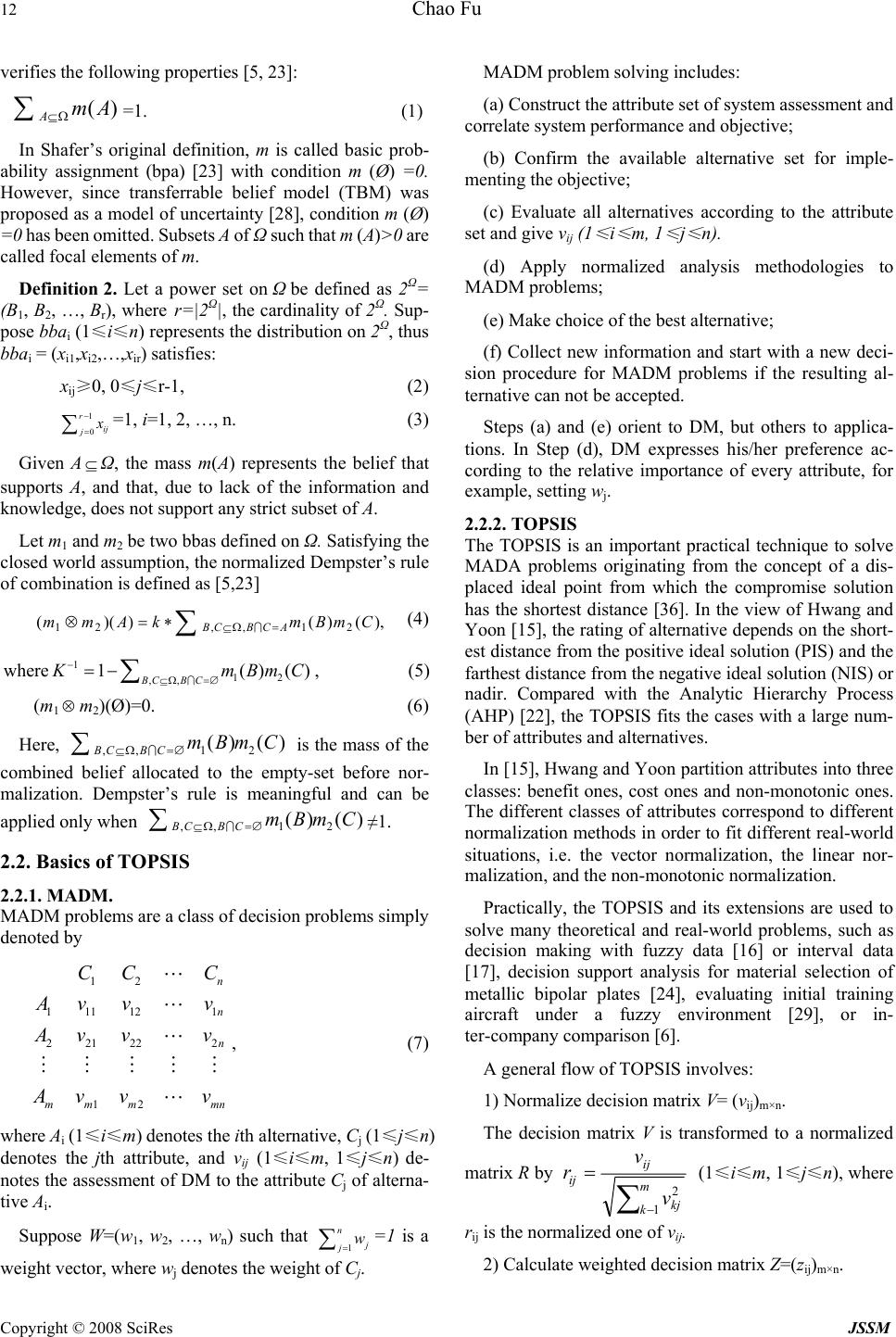 12 Chao Fu Copyright © 2008 SciRes JSSM verifies the following properties [5, 23]: () AmA ⊆Ω ∑=1. (1) In Shafer’s original definition, m is called basic prob- ability assignment (bpa) [23] with condition m (Ø) =0. However, since transferrable belief model (TBM) was proposed as a model of uncertainty [28], condition m (Ø) =0 has been omitted. Subsets A of Ω such that m (A)>0 are called focal elements of m. Definition 2. Let a power set on Ω be defined as 2Ω= (B1, B2, …, Br), where r=|2Ω|, the cardinality of 2Ω. Sup- pose bbai (1≤i≤n) represents the distribution on 2Ω, thus bbai = (xi1,xi2,…,xir) satisfies: xij≥0, 0≤j≤r-1, (2) 1 0 r ij j x − = ∑=1, i=1, 2, …, n. (3) Given A⊆Ω, the mass m(A) represents the belief that supports A, and that, due to lack of the information and knowledge, does not support any strict subset of A. Let m1 and m2 be two bbas defined on Ω. Satisfying the closed world assumption, the normalized Dempster’s rule of combination is defined as [5,23] ),()())(( 21,,21 CmBmkAmm ACBCB ∑=Ω⊆ ∗=⊗ I (4) where 1 12 ,, 1()() BCB C K mBmC − ⊆Ω =∅ =− ∑I, (5) (m1⊗m2)(Ø)=0. (6) Here, ,,1 2 () () BCB CmBmC ⊆Ω =∅ ∑I is the mass of the combined belief allocated to the empty-set before nor- malization. Dempster’s rule is meaningful and can be applied only when ,,1 2 () () BCB CmBmC ⊆Ω =∅ ∑I≠1. 2.2. Basics of TOPSIS 2.2.1. MAD M. MADM problems are a class of decision problems simply denoted by 12 11112 1 22122 2 12 n n n mm mmn CC C A vv v A vv v A vv v L L L MMMMM L , (7) where Ai (1≤i≤m) denotes the ith alternative, Cj (1≤j≤n) denotes the jth attribute, and vij (1≤i≤m, 1≤j≤n) de- notes the assessment of DM to the attribute Cj of alterna- tive Ai. Suppose W=(w1, w2, …, wn) such that 1 n j jw = ∑=1 is a weight vector, where wj denotes the weight of Cj. MADM problem solving includes: (a) Construct the attribute set of system assessment and correlate system performance and objective; (b) Confirm the available alternative set for imple- menting the objective; (c) Evaluate all alternatives according to the attribute set and give vij (1 ≤ i ≤ m, 1 ≤ j ≤ n). (d) Apply normalized analysis methodologies to MADM problems; (e) Make choice of the best alternative; (f) Collect new information and start with a new deci- sion procedure for MADM problems if the resulting al- ternative can not be accepted. Steps (a) and (e) orient to DM, but others to applica- tions. In Step (d), DM expresses his/her preference ac- cording to the relative importance of every attribute, for example, setting wj. 2.2.2. TOPSIS The TOPSIS is an important practical technique to solve MADA problems originating from the concept of a dis- placed ideal point from which the compromise solution has the shortest distance [36]. In the view of Hwang and Yoon [15], the rating of alternative depends on the short- est distance from the positive ideal solution (PIS) and the farthest distance from the negative ideal solution (NIS) or nadir. Compared with the Analytic Hierarchy Process (AHP) [22], the TOPSIS fits the cases with a large num- ber of attributes and alternatives. In [15], Hwang and Yoon partition attributes into three classes: benefit ones, cost ones and non-monotonic ones. The different classes of attributes correspond to different normalization methods in order to fit different real-world situations, i.e. the vector normalization, the linear nor- malization, and the non-monotonic normalization. Practically, the TOPSIS and its extensions are used to solve many theoretical and real-world problems, such as decision making with fuzzy data [16] or interval data [17], decision support analysis for material selection of metallic bipolar plates [24], evaluating initial training aircraft under a fuzzy environment [29], or in- ter-company comparison [6]. A general flow of TOPSIS involves: 1) Normalize decision matrix V= (vij)m×n. The decision matrix V is transformed to a normalized matrix R by ∑− =m kkj ij ij v v r 1 2 (1≤i≤m, 1≤j≤n), where rij is the normalized one of vij. 2) Calculate weighted decision matrix Z=(zij)m×n. 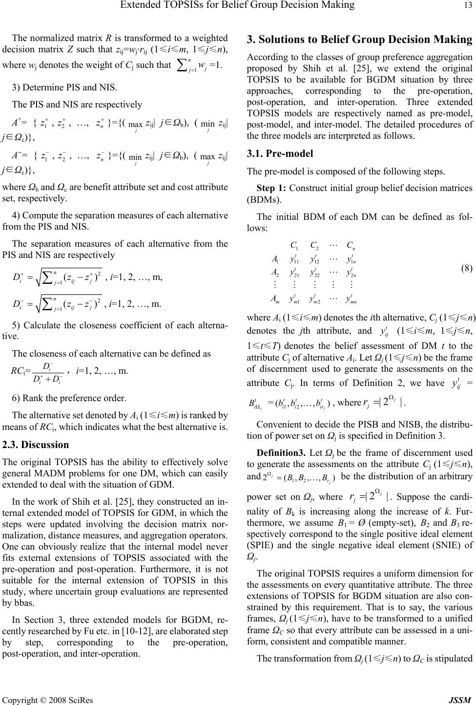 Extended TOPSISs for Belief Group Decision Making 13 Copyright © 2008 SciRes JSSM The normalized matrix R is transformed to a weighted decision matrix Z such that zij=wj·rij (1≤i≤m, 1≤j≤n), where wj denotes the weight of Cj such that 1 n j jw = ∑=1. 3) Determine PIS and NIS. The PIS and NIS are respectively A+= {1 z+,2 z+, …, n z+}={( max j zij| j∈Ωb), (min j zij| j∈Ωc)}, A - = {1 z−,2 z−, …, n z−}={( min j zij| j∈Ωb), (max j zij| j∈Ωc)}, where Ωb and Ωc are benefit attribute set and cost attribute set, respectively. 4) Compute the separation measures of each alternative from the PIS and NIS. The separation measures of each alternative from the PIS and NIS are respectively 2 1() n iijj j Dzz ++ = =− ∑, i=1, 2, …, m, 2 1() n iijj j Dzz −− = =− ∑, i=1, 2, …, m. 5) Calculate the closeness coefficient of each alterna- tive. The closeness of each alternative can be defined as RCi=i ii D D D − +− + ,i=1, 2, …, m. 6) Rank the preference order. The alternative set denoted by Ai (1≤i≤m) is ranked by means of RCi, which indicates what the best alternative is. 2.3. Discussion The original TOPSIS has the ability to effectively solve general MADM problems for one DM, which can easily extended to deal with the situation of GDM. In the work of Shih et al. [25], they constructed an in- ternal extended model of TOPSIS for GDM, in which the steps were updated involving the decision matrix nor- malization, distance measures, and aggregation operators. One can obviously realize that the internal model never fits external extensions of TOPSIS associated with the pre-operation and post-operation. Furthermore, it is not suitable for the internal extension of TOPSIS in this study, where uncertain group evaluations are represented by bbas. In Section 3, three extended models for BGDM, re- cently researched by Fu etc. in [10-12], are elaborated step by step, corresponding to the pre-operation, post-operation, and inter-operation. 3. Solutions to Belief Group Decision Making According to the classes of group preference aggregation proposed by Shih et al. [25], we extend the original TOPSIS to be available for BGDM situation by three approaches, corresponding to the pre-operation, post-operation, and inter-operation. Three extended TOPSIS models are respectively named as pre-model, post-model, and inter-model. The detailed procedures of the three models are interpreted as follows. 3.1. Pre-model The pre-model is composed of the following steps. Step 1: Construct initial group belief decision matrices (BDMs). The initial BDM of each DM can be defined as fol- lows: 12 11112 1 22122 2 12 n tt t n tt t n tt t mm mmn CC C A yyy A yy y A yyy L L L MM MMM L (8) where Ai (1≤i≤m) denotes the ith alternative, Cj (1≤j≤n) denotes the jth attribute, and t ij y (1≤i≤m, 1≤j≤n, 1≤t≤T) denotes the belief assessment of DM t to the attribute Cj of alternative Ai. Let Ωj (1≤j≤n) be the frame of discernment used to generate the assessments on the attribute Cj. In terms of Definition 2, we have t ij y = j t i B Ω =12 (, ,,) j tt t ii ir bb bK, where|2 | j j rΩ =. Convenient to decide the PISB and NISB, the distribu- tion of power set on Ωj is specified in Definition 3. Definition3. Let Ωj be the frame of discernment used to generate the assessments on the attribute Cj (1≤j≤n), and 12 2(,,,) j j r B BB Ω=K be the distribution of an arbitrary power set on Ωj, where |2 | j j rΩ =. Suppose the cardi- nality of Bk is increasing along the increase of k. Fur- thermore, we assume B1 = Ø (empty-set), B2 and B3 re- spectively correspond to the single positive ideal element (SPIE) and the single negative ideal element (SNIE) of Ωj. The original TOPSIS requires a uniform dimension for the assessments on every quantitative attribute. The three extensions of TOPSIS for BGDM situation are also con- strained by this requirement. That is to say, the various frames, Ωj (1≤j≤n), have to be transformed to a unified frame ΩC so that every attribute can be assessed in a uni- form, consistent and compatible manner. The transformation from Ωj (1≤j≤n) to ΩC is stipulated 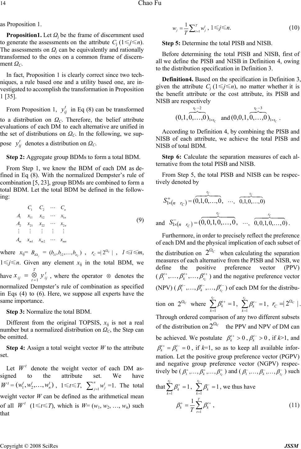 14 Chao Fu Copyright © 2008 SciRes JSSM as Proposition 1. Proposition1. Let Ωj be the frame of discernment used to generate the assessments on the attribute Cj (1≤j≤n). The assessments on Ωj can be equivalently and rationally transformed to the ones on a common frame of discern- ment ΩC. In fact, Proposition 1 is clearly correct since two tech- niques, a rule based one and a utility based one, are in- vestigated to accomplish the transformation in Proposition 1 [35]. From Proposition 1, t ij y in Eq (8) can be transformed to a distribution on ΩC. Therefore, the belief attribute evaluations of each DM to each alternative are unified in the set of distributions on ΩC. In the following, we sup- pose t ij y denotes a distribution on ΩC. Step 2: Aggregate group BDMs to form a total BDM. From Step 1, we know the BDM of each DM as de- fined in Eq (8). With the normalized Dempster’s rule of combination [5, 23], group BDMs are combined to form a total BDM. Let the total BDM be defined in the follow- ing: 12 11112 1 221222 12 n n n mm mmn CC C Ax xx Ax xx Ax xx L L L MMMMM L (9) where xij=j i B Ω=12 (, ,,) C ii ir bb bK, |2 | C C rΩ =, 1 ≤ i ≤ m, 1≤j≤n. Given any element xij in the total BDM, we have 1 Tt ij ij t xy = =⊗ , where the operator ⊗ denotes the normalized Dempster’s rule of combination as specified in Eqs (4) to (6). Here, we suppose all experts have the same importance. Step 3: Normalize the total BDM. Different from the original TOPSIS, xij is not a real number but a normalized distribution on ΩC, the Step can be omitted. Step 4: Assign a total weight vector W to the attribute set. Let t W denote the weight vector of each DM as- signed to the attribute set. We have t W=12 (, ,,) tt t n ww wK, 1≤t≤T, 1 nt j jw = ∑=1. The total weight vector W can be defined as the arithmetical mean of all t W (1≤t≤T), which is W= (w1, w2, …, wn) such that 1 1Tt j j t ww T= =∑, 1≤j≤n. (10) Step 5: Determine the total PISB and NISB. Before determining the total PISB and NISB, first of all we define the PISB and NISB in Definition 4, owing to the distribution specification in Definition 3. Definition4. Based on the specification in Definition 3, given the attribute Cj (1≤j≤n), no matter whether it is the benefit attribute or the cost attribute, its PISB and NISB are respectively C C r2 1r (0,1,0, ,0) − × 678 K and C C r3 1r (0,0,1, 0,,0 ) − × 678 K. According to Definition 4, by combining the PISB and NISB of each attribute, we achieve the total PISB and NISB of total BDM. Step 6: Calculate the separation measures of each al- ternative from the total PISB and NISB. From Step 5, the total PISB and NISB can be respec- tively denoted by () + ×C rn S1=(0,1,0, ,0, C r 6 4748 K ,L 0,1,0, ,0) C r 647 48 K and () − ×C rn S1=(0,0,1,0, ,0, C r 6 447 448 K ,L 0,0,1, 0,, 0) C r 6447 448 K. Furthermore, in order to precisely reflect the preference of each DM and the physical implication of each subset of the distribution on 2C Ω when calculating the separation measures of each alternative from the PISB and NISB, we define the positive preference vector (PPV) (1,, ,, C ttt kr β ββ + ++ KK ) and the negative preference vector (NPV) (1,, ,, C ttt kr βββ − −− KK ) of each DM for the distribu- tion on C Ω 2 where 1 1 C r t k k β + = = ∑, 1 1 C r t k k β − = = ∑, |2 | C C rΩ =. Through ordered comparison of any two different subsets of the distribution onC Ω 2 the PPV and NPV of DM can be achieved. We postulate 0 t k β +>,0 t k β −>, if k>1, and 0 tt kk ββ +− = =, if k=1, so as to keep all available infor- mation. Let the positive group preference vector (PGPV) and negative group preference vector (NGPV) respec- tively be (1,, ,, C kr β ββ + ++ KK) and (1,,,, C kr β ββ −−− KK) such that 1 1 C r k k β + = = ∑, 1 1 C r k k β − = = ∑, we thus have 1 1T t kk t T β β + + = = ∑ , (11) 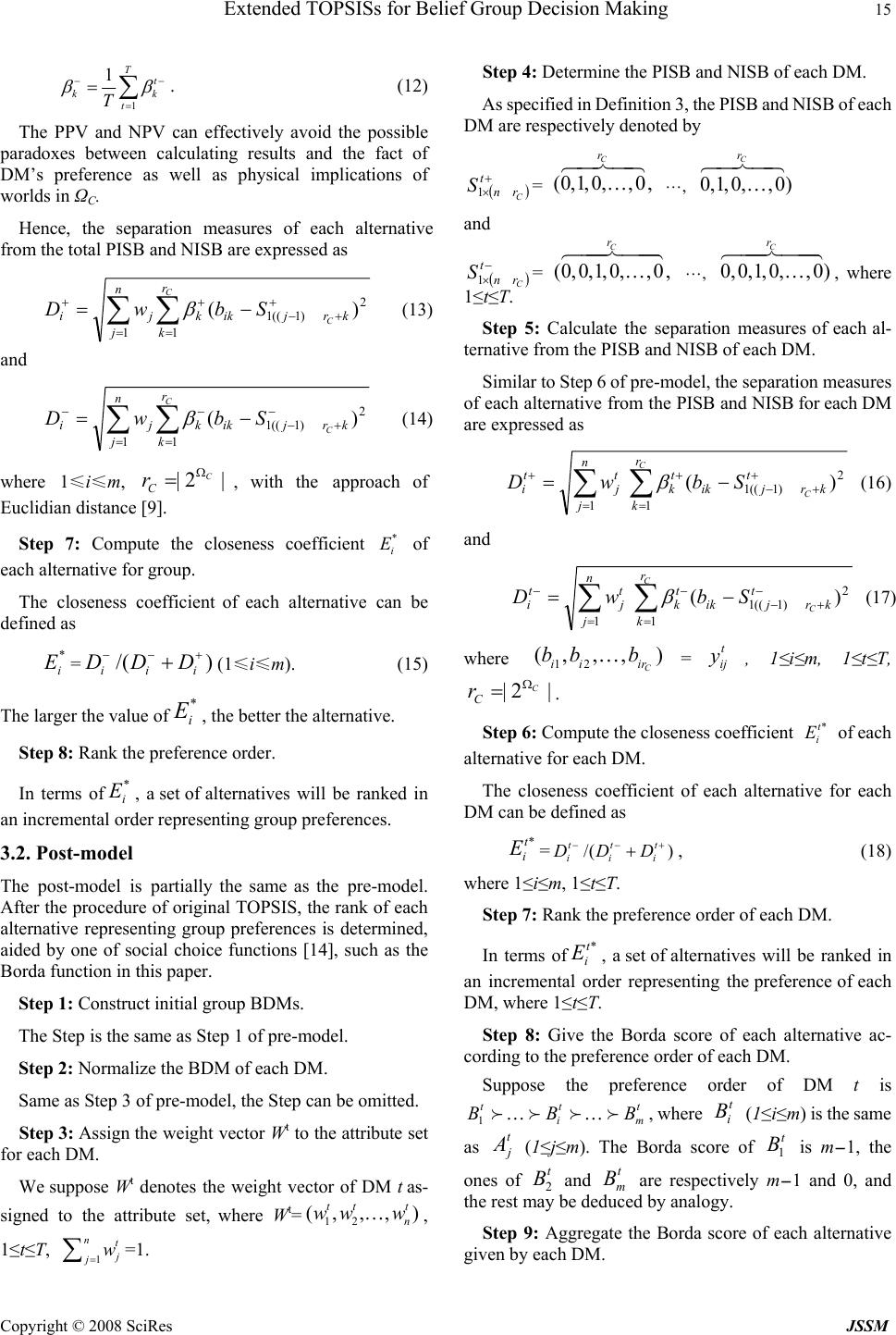 Extended TOPSISs for Belief Group Decision Making 15 Copyright © 2008 SciRes JSSM 1 1T t kk t T β β −− = =∑. (12) The PPV and NPV can effectively avoid the possible paradoxes between calculating results and the fact of DM’s preference as well as physical implications of worlds in ΩC. Hence, the separation measures of each alternative from the total PISB and NISB are expressed as 2 )1((1 11 )( + +− = + = +−= ∑∑ krjik r k k n j ji C C SbwD β (13) and 2 )1((1 11 )( − +− = − = −−= ∑∑ krjik r k k n j ji C C SbwD β (14) where 1≤i≤m, |2 | C C rΩ =, with the approach of Euclidian distance [9]. Step 7: Compute the closeness coefficient * i E of each alternative for group. The closeness coefficient of each alternative can be defined as * i E =/( ) ii i DD D −− + +(1≤i≤m). (15) The larger the value of* i E , the better the alternative. Step 8: Rank the preference order. In terms of* i E , a set of alternatives will be ranked in an incremental order representing group preferences. 3.2. Post-model The post-model is partially the same as the pre-model. After the procedure of original TOPSIS, the rank of each alternative representing group preferences is determined, aided by one of social choice functions [14], such as the Borda function in this paper. Step 1: Construct initial group BDMs. The Step is the same as Step 1 of pre-model. Step 2: Normalize the BDM of each DM. Same as Step 3 of pre-model, the Step can be omitted. Step 3: Assign the weight vector Wt to the attribute set for each DM. We suppose Wt denotes the weight vector of DM t as- signed to the attribute set, where Wt=12 (, ,,) tt t n ww wK, 1≤t≤T, 1 nt j jw = ∑=1. Step 4: Determine the PISB and NISB of each DM. As specified in Definition 3, the PISB and NISB of each DM are respectively denoted by () + × t rn C S1= (0,1,0, ,0, C r 6 4748 K ,L 0,1, 0,, 0) C r 64748 K and () − × t rn C S1= (0,0,1,0, ,0, C r 6 447448 K ,L 0, 0,1, 0,, 0) C r 6447448 K, where 1≤t≤T. Step 5: Calculate the separation measures of each al- ternative from the PISB and NISB of each DM. Similar to Step 6 of pre-model, the separation measures of each alternative from the PISB and NISB for each DM are expressed as 2 )1((1 11 )( + +− = + = +−=∑∑ t krjik r k t k n j t j t iC C SbwD β (16) and 2 )1((1 11 )( − +− = − = −−=∑∑ t krjik r k t k n j t j t iC C SbwD β (17) where 12 (,, ,) C ii ir bb bK=t ij y, 1≤i≤m, 1≤t≤T, |2 | C C rΩ =. Step 6: Compute the closeness coefficient *t i E of each alternative for each DM. The closeness coefficient of each alternative for each DM can be defined as *t i E =/( ) ttt ii i DDD − −+ +, (18) where 1≤i≤m, 1≤t≤T. Step 7: Rank the preference order of each DM. In terms of*t i E , a set of alternatives will be ranked in an incremental order representing the preference of each DM, where 1≤t≤T. Step 8: Give the Borda score of each alternative ac- cording to the preference order of each DM. Suppose the preference order of DM t is 1 ttt im BBBfKf fKf , where t i B (1≤i≤m) is the same as t j A (1≤j≤m). The Borda score of 1 t B is m - 1, the ones of 2 t B and t m B are respectively m - 1 and 0, and the rest may be deduced by analogy. Step 9: Aggregate the Borda score of each alternative given by each DM.  16 Chao Fu Copyright © 2008 SciRes JSSM Let the Borda score vectors of each alternative repre- senting the preference of DM t and group preferences be respectively (1,,,, ttt im SSSKK) and (1,,,, im SSSKK). We have 1 T t ii t SS = =∑, 1≤i≤m. (19) Step 10: Rank the preference order for group. According to (1,,,, im SSSKK), we rank the prefer- ence order of a set of alternatives for group. 3.3. Inter-model The inter-model is similar to the internal TOPSIS model of Shih et al. [25]. It combines the individual separation measures of each alternative from the PISB and NISB to form group measures within the TOPSIS procedure. The first five Steps of inter-model are the same as Steps 1 to 5 of post-model. Step 6: Combine the individual measures of each al- ternative from the PISB and NISB to form group meas- ures. From Step 5 of post-model, we achieve the individual measures of each alternative from the PISB and NISB, which are respectively t i D + and t i D − (1≤i≤m, 1≤t≤T). Thus, the group measures of each alternative are respec- tively 1 Tt ii t D D ++ = =⊕ (20) and 1 Tt ii t D D −− = =⊕ . (21) The operator ⊕ can be the arithmetical mean, the geometric mean, or their modifications. In this paper, the arithmetical mean is our choice. Steps 7 and 8 are the same as Steps 7 and 8 of pre-model. As mentioned above, three extended models are similar to each other in many Steps. The main differences lie in the aggregation of group preferences. In the pre-model, thanks to two strategies of Dempster’s rule modification (e.g. [8, 19, 26-27, 32-33]) and source modification (e.g. [7, 13, 21]) aiming at combining con- flicting beliefs, the preference conflicts between different DMs can be effectively dealt with. In the post-model, some social choice functions [14] can be selected to guarantee group preferences aggregation is rational and available in different applications. In the inter-model, the arithmetical mean, the geometric mean, or their modifi- cations are used to aggregate the individual separation measures of each alternative from the PISB and NISB. In practice, how to select the appropriate extended model depends on how to select the appropriate approach to aggregating group preferences, which is the most suitable one for real-world problems. 4. Numerical Example To clearly illustrate the procedures of three extended models, a numerical example is shown as follows. From Tables 1 to 3, one can know initial group BDMs, and the preference vectors and weight vector of each DM. There are two attributes, three alternatives, and three DMs in this example. Two attributes C1 and C2 are the benefit one and the cost one, respectively. Suppose Ω1= {good, common}, Ω2= {small, big, common}, ΩC= {first, second, third}, according to Proposition 1, the assess- ments on Ω1 and Ω2 can be equivalently transformed to the ones on ΩC. In terms of Definition 3, the power set on ΩC is {{Ø}, {first}, {third}, {second}, {first, third}, {first, second}, {second, third}, {first, second, third}}. As specified in Definition 4, the PISB and NISB are respectively (0,1,0,0,0,0,0,0,0,1,0,0,0,0,0,0) and (0,0,1,0, 0,0,0,0,0,0,1,0,0,0,0,0). The decision procedures of three extended models will be presented as follows. In the pre-model, group belief evaluations are firstly combined to form the total BDM displayed in Table 4, with the normalized Dempster’s rule of combination. Afterwards, according to Eq (10), the total weight vector W= (0.6, 0.4) is generated from the weight vectors in Table 3. Based on the data in Table 2, the PGPV and NGPV are computed respectively as (0,0.03,0.207,0.092, 0.207,0.05,0.207,0.207) and (0,0.384,0.055,0.163,0.055, 0.233,0.055,0.055), in terms of Eqs (11) and (12). With the above results, the total separation measures and the closeness coefficient of each alternative are ob- tained in Table 5, according to Eqs (13) to (15). From Table 5, the preference order of three alternatives is known to be A1fA3fA2, where the notation “f” means “prior”. In the post-model, first of all the individual separation measures and the closeness coefficient of each alternative are computed in Table 6. The Borda score and rank of each alternative for group are generated from the data in Table 6 and shown in Table 7. According to Table 7, three alternatives are ranked by the preference order A1fA2=A3. In the inter-model, the separation measures and close- ness coefficient of each alternative for group are achieved in Table 8, on the basis of the data in Table 6. Three alternatives are ranked with the preference order A1fA2fA3 according to Table 8. 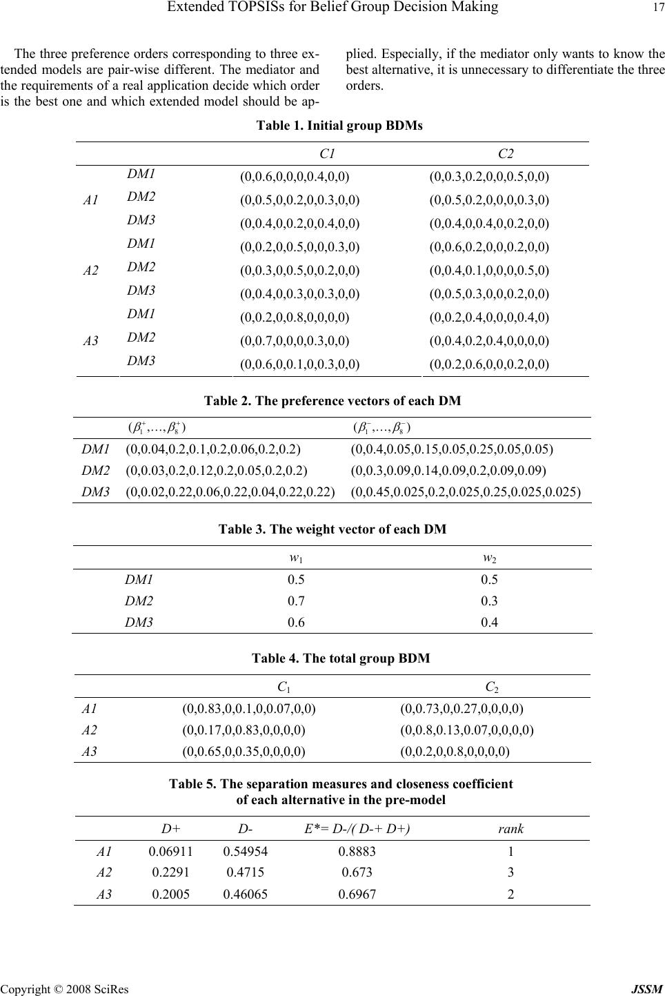 Extended TOPSISs for Belief Group Decision Making 17 Copyright © 2008 SciRes JSSM The three preference orders corresponding to three ex- tended models are pair-wise different. The mediator and the requirements of a real application decide which order is the best one and which extended model should be ap- plied. Especially, if the mediator only wants to know the best alternative, it is unnecessary to differentiate the three orders. Table 1. Initial group BDMs C1 C2 DM1 (0,0.6,0,0,0,0.4,0,0) (0,0.3,0.2,0,0,0.5,0,0) DM2 (0,0.5,0,0.2,0,0.3,0,0) (0,0.5,0.2,0,0,0,0.3,0) A1 DM3 (0,0.4,0,0.2,0,0.4,0,0) (0,0.4,0,0.4,0,0.2,0,0) DM1 (0,0.2,0,0.5,0,0,0.3,0) (0,0.6,0.2,0,0,0.2,0,0) DM2 (0,0.3,0,0.5,0,0.2,0,0) (0,0.4,0.1,0,0,0,0.5,0) A2 DM3 (0,0.4,0,0.3,0,0.3,0,0) (0,0.5,0.3,0,0,0.2,0,0) DM1 (0,0.2,0,0.8,0,0,0,0) (0,0.2,0.4,0,0,0,0.4,0) DM2 (0,0.7,0,0,0,0.3,0,0) (0,0.4,0.2,0.4,0,0,0,0) A3 DM3 (0,0.6,0,0.1,0,0.3,0,0) (0,0.2,0.6,0,0,0.2,0,0) Table 2. The preference vectors of each DM 18 (,,) β β ++ K 18 (,,) β β − − K DM1 (0,0.04,0.2,0.1,0.2,0.06,0.2,0.2) (0,0.4,0.05,0.15,0.05,0.25,0.05,0.05) DM2 (0,0.03,0.2,0.12,0.2,0.05,0.2,0.2) (0,0.3,0.09,0.14,0.09,0.2,0.09,0.09) DM3 (0,0.02,0.22,0.06,0.22,0.04,0.22,0.22) (0,0.45,0.025,0.2,0.025,0.25,0.025,0.025) Table 3. The w e ight vector of each DM w1 w2 DM1 0.5 0.5 DM2 0.7 0.3 DM3 0.6 0.4 Table 4. The total group BDM C1 C2 A1 (0,0.83,0,0.1,0,0.07,0,0) (0,0.73,0,0.27,0,0,0,0) A2 (0,0.17,0,0.83,0,0,0,0) (0,0.8,0.13,0.07,0,0,0,0) A3 (0,0.65,0,0.35,0,0,0,0) (0,0.2,0,0.8,0,0,0,0) Table 5. The separation measures and closeness coefficient of each alternative in the pre-model D+ D- E*= D-/( D-+ D+) rank A1 0.06911 0.54954 0.8883 1 A2 0.2291 0.4715 0.673 3 A3 0.2005 0.46065 0.6967 2 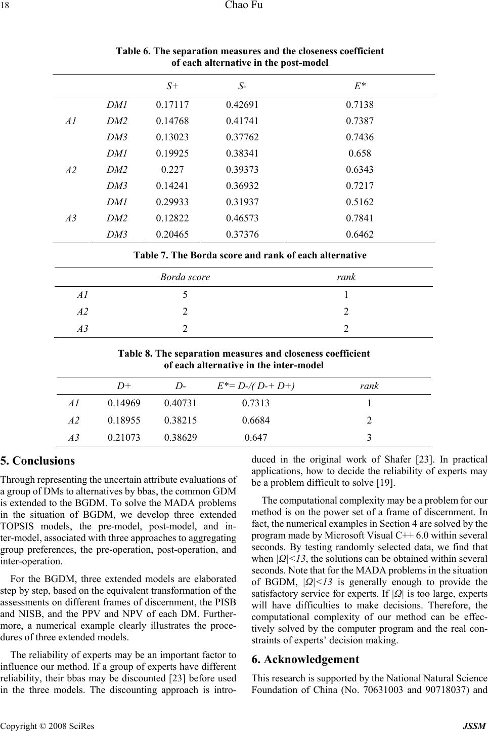 18 Chao Fu Copyright © 2008 SciRes JSSM Table 6. The separation measures and the closeness coefficient of each alternative in the post-model S+ S- E* DM1 0.17117 0.42691 0.7138 DM2 0.14768 0.41741 0.7387 A1 DM3 0.13023 0.37762 0.7436 DM1 0.19925 0.38341 0.658 DM2 0.227 0.39373 0.6343 A2 DM3 0.14241 0.36932 0.7217 DM1 0.29933 0.31937 0.5162 DM2 0.12822 0.46573 0.7841 A3 DM3 0.20465 0.37376 0.6462 Table 7. The Borda score and rank of each alternative Borda score rank A1 5 1 A2 2 2 A3 2 2 Table 8. The separation measures and closeness coefficient of each alternative in the inter-model D+ D- E*= D-/( D-+ D+) rank A1 0.14969 0.407310.7313 1 A2 0.18955 0.382150.6684 2 A3 0.21073 0.386290.647 3 5. Conclusions Through representing the uncertain attribute evaluations of a group of DMs to alternatives by bbas, the common GDM is extended to the BGDM. To solve the MADA problems in the situation of BGDM, we develop three extended TOPSIS models, the pre-model, post-model, and in- ter-model, associated with three approaches to aggregating group preferences, the pre-operation, post-operation, and inter-operation. For the BGDM, three extended models are elaborated step by step, based on the equivalent transformation of the assessments on different frames of discernment, the PISB and NISB, and the PPV and NPV of each DM. Further- more, a numerical example clearly illustrates the proce- dures of three extended models. The reliability of experts may be an important factor to influence our method. If a group of experts have different reliability, their bbas may be discounted [23] before used in the three models. The discounting approach is intro- duced in the original work of Shafer [23]. In practical applications, how to decide the reliability of experts may be a problem difficult to solve [19]. The computational complexity may be a problem for our method is on the power set of a frame of discernment. In fact, the numerical examples in Section 4 are solved by the program made by Microsoft Visual C++ 6.0 within several seconds. By testing randomly selected data, we find that when |Ω|<13, the solutions can be obtained within several seconds. Note that for the MADA problems in the situation of BGDM, |Ω|<13 is generally enough to provide the satisfactory service for experts. If |Ω| is too large, experts will have difficulties to make decisions. Therefore, the computational complexity of our method can be effec- tively solved by the computer program and the real con- straints of experts’ decision making. 6. Acknowledgement This research is supported by the National Natural Science Foundation of China (No. 70631003 and 90718037) and 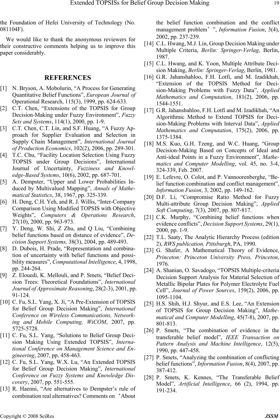 Extended TOPSISs for Belief Group Decision Making 19 Copyright © 2008 SciRes JSSM the Foundation of Hefei University of Technology (No. 081104F). We would like to thank the anonymous reviewers for their constructive comments helping us to improve this paper considerably. REFERENCES [1] N. Bryson, A. Mobolurin, “A Process for Generating Quantitative Belief Functions”, European Journal of Operational Research, 115(3), 1999, pp. 624-633. [2] C.T. Chen, “Extensions of the TOPSIS for Group Decision-Making under Fuzzy Environment”, Fuzzy Sets and Systems, 114(1), 2000, pp. 1-9. [3] C.T. Chen, C.T. Lin, and S.F. Huang, “A Fuzzy Ap- proach for Supplier Evaluation and Selection in Supply Chain Management”, International Journal of Production Economics, 102(2), 2006, pp. 289-301. [4] T.C. Chu, “Facility Location Selection Using Fuzzy TOPSIS under Group Decisions”, International Journal of Uncertainty, Fuzziness and Knowl- edge-Based Systems, 10(6), 2002, pp. 687-701. [5] A. Dempster, “Upper and Lower Probabilities In- duced by Multivalued Mapping”, Annals of Mathe- matical Statistics, 38, 1967, pp. 325-339. [6] H. Deng, C.H. Yeh, and R. J. Willis, “Inter-Company Comparison Using Modified TOPSIS with Objective Weights”, Computers & Operations Research, 27(10), 2000, pp. 963-973. [7] Y. Deng, W. Shi, Z Zhu, and Q Liu, “Combining belief functions based on distance of evidence”, De- cision Support Systems, 38(3), 2004, pp. 489-493. [8] D. Dubois, H. Prade, “Representation and combina- tion of uncertainty with belief functions and possi- bility measures”, Computational Intelligence, 4, 1998, pp. 244-264. [9] Z. Elouedi, K. Mellouli, and P. Smets, “Belief Deci- sion Trees: Theoretical Foundations”, International Journal of Approximate Reasoning, 28(2-3), 2001, pp. 91-124. [10] C. Fu, S.L. Yang, X. Ji, “A Pre-Extension of TOPSIS for Belief Group Decision Making”, International Conference on Wireless Communications, Network- ing and Mobile Computing, WiCOM, 2007, pp. 5725-5728. [11] C. Fu, S.L. Yang, “Solutions to Belief Group Deci- sion Making Using Extended TOPSIS”, Interna- tional Conference on Management Science and En- gineering, 2007, pp. 458-463. [12] C. Fu, S.L. Yang, W.X. Lu, “An Extended TOPSIS for Belief Group Decision Making”, International Conference on Fuzzy Systems and Knowledge Dis- covery, 2007, pp. 551-555. [13] R. Haenni, “Are alternatives to Dempster’s rule of combination real alternatives? Comments on ‘About the belief function combination and the conflict management problem’”, Information Fusion, 3(4), 2002, pp. 237-239. [14] C.L. Hwang, M.J. Lin, Group Decision Making under Multiple Criteria, Berlin: Springer-Verlag, Berlin, 1987. [15] C.L. Hwang, and K. Yoon, Multiple Attribute Deci- sion Making, Berlin: Springer-Verlag, Berlin, 1981. [16] G.R. Jahanshahloo, F.H. Lotfi, and M. Izadikhah, “Extension of the TOPSIS Method for Deci- sion-Making Problems with Fuzzy Data”, Applied Mathematics and Computation, 181(2), 2006, pp. 1544-1551. [17] G.R. Jahanshahloo, F.H. Lotfi and M. Izadikhah, “An Algorithmic Method to Extend TOPSIS for Deci- sion-Making Problems with Interval Data”, Applied Mathematics and Computation, 175(2), 2006, pp. 1375-1384. [18] M.S. Kuo, G.H. Tzeng, and W.C. Huang, “Group Decision-Making Based on Concepts of Ideal and Anti-ideal Points in a Fuzzy Environment”, Mathe- matics and Computer Modelling, vol. 45, no. 3-4, 324-339, Feb. 2007. [19] E. Lefevre, O. Colot, and P. Vannoorenberghe, “Be- lief function combination and conflict management”, Information Fusion, 3, 2002, pp. 149-162. [20] D.F. Li, “Compromise Ratio Method for Fuzzy Multi-attribute Group Decision Making”, Applied Soft Computing, 7(3), 2007, pp. 807-817. [21] C.K. Murphy, “Combining belief functions when evidence conflicts”, Decision Support Systems, 29(1), 2000, pp. 1-9. [22] T.L. Saaty, The Analytic Hierarchy Process (edition 2), RWS publication, Pittsburgh, PA, 1990. [23] G. Shafer, A Mathematical Theory of Evidence, Princeton: Princeton University Press, Princeton, 1976. [24] A. Shanian, O. Savadogo, “TOPSIS Multiple-criteria Decision Support Analysis for Material Selection of Metallic Bipolar Plates for Polymer Electrolyte Fuel Cell”, Journal of Power Sources, 159(2), 2006, pp. 1095-1104. [25] H.S. Shih, H.J. Shyur, and E.S. Lee, “An Extension of TOPSIS for Group Decision Making”, Mathe- matical and Computer Modelling, 45(7-8), 2007, pp. 801-813. [26] P. Smets, “The combination of evidence in the transferable belief model”, IEEE Transaction on Pattern Analysis and Machine Intelligence, 12(5), 1990, pp. 447-458. [27] P. Smets, “Analyzing the combination of conflicting belief functions”, Information Fusion, 8(4), 2007, pp. 387-412. [28] P. Smets, K. Kennes, “The Transferable Belief Model”, Artificial Intelligence, 66 (2), 1994, pp. 191-234.  20 Chao Fu Copyright © 2008 SciRes JSSM [29] T.C. Wang, T.H. Chang, “Application of TOPSIS in Evaluating Initial Training Aircraft under a Fuzzy Environment”, Expert Systems with Applications, 33(4), 2007, pp. 870-880. [30] Y.M. Wang, Y. Luo, and Z.S. Hua, “A Note on Group Decision-Making Based on Concepts of Ideal and Anti-ideal Points in a Fuzzy Environment”, Mathematical and Computer Modelling, 46(9-10), 2007, pp. 1256-1264. [31] S.K.M. Wong, P. Lingras, “Representation of Qualitative User Preference by Quantitative Belief Functions”, IEEE Transactions on Knowledge and Data Engineering, 6(1), 1994, pp. 72-78. [32] R.R. Yager, “On the Dempster-Shafer Framework and New Combination Rules”, Information Sciences, 41(2), 1987, pp. 93-137. [33] R.R. Yager, “Quasi-associative operations in the combination of evidence”, Kybernetes, 16, 1987, 37-41. [34] A.Ben Yaghlane, T. Denoeux, and K. Mellouli, “Constructing Belief Functions from Qualitative Expert Opinions”, Information and Communication Technologies, ICTTA’06, 1, 2006, pp. 1363-1368. [35] J.B. Yang, “Rule and Utility Based Evidential Rea- soning Approach for Multiattribute Decision Analy- sis under Uncertainties”, European Journal of Op- erational Research, 131, 2001, pp. 31-61. [36] M. Zeleny, “A Concept of Compromise Solutions and the Method of the Displaced Ideal”, Computers and Operations Research, 1(3-4), 1974, pp. 479-496. AUTHOR’S BI OG R A PHY Chao Fu received his M.S. degree in Mechanical and Electronic Engineering from Huazhong University of Science and Technology, Wuhan, Hubei, China in 2003. He joined Hefei University of Technology, where he is currently a lecturer at School of Management. He is a researcher of Key Laboratory of Process Optimization and Intelligent Decision-making, Ministry of Education, in the same school. His research interests include decision science and technology, information systems and engineering, and the simulation of complex decision task. |

