 Journal of Signal and Information Processing, 2013, 4, 274-281 http://dx.doi.org/10.4236/jsip.2013.43035 Published Online August 2013 (http://www.scirp.org/journal/jsip) Generalized Parseval’s Theorem on Fractional Fourier Transform for Discrete Signals and Filtering of LFM Signals Xiaotong Wang1, Guanlei Xu1,2, Yue Ma1*, Lijia Zhou2, Longtao Wang2 1Automation Department of Dalian Naval Academy, Dalian, China; 2Ocean Department of Dalian Naval Academy, Dalian, China. Email: *mayue0205@163.com Received June 23rd, 2013; revised July 23rd, 2013; accepted August 13th, 2013 Copyright © 2013 Xiaotong Wang et al. This is an open access article distributed under the Creative Commons Attribution License, which permits unrestricted use, distribution, and reproduction in any medium, provided the original work is properly cited. ABSTRACT This paper investigates the generalized Parseval’s theorem of fractional Fourier transform (FRFT) for concentrated data. Also, in the framework of multiple FRFT domains, Parseval’s theorem reduces to an inequality with lower and upper bounds associated with FRFT parameters, named as generalized Parseval’s theorem by us. These results theoretically provide potential valuable applications in filtering, and examples of filtering for LFM signals in FRFT domains are demonstrated to support the derived conclusions. Keywords: Discrete Fractional Fourier Transform (DFRFT); Uncertainty Principle; Frequency-Limiting Operator; Linear Frequency-Modulation (LFM) Signal; Filtering 1. Introduction In signal processing, data concentration is often consid- ered carefully via the uncertainty principle [1-8]. In con- tinuous signals, the supports are assumed to be , , based on which various uncertainty relations [1,2,9-27] have been presented. However, Parseval’s theorem has not been discussed for multiple FRFT domains anywhere else. As the rotation of the traditional FT [28], FRFT [5,6,22,23,29] has some special properties with its trans- formed parameter and sometimes yields the better result such as LFM detection [30]. Readers can see more de- tails on FRFT in [6] and [31] and so on. Another impor- tant issue in signal processing is filtering. Filtering in frequency domain is widely employed for its easy im- plementation and high efficiency in many cases [5,32]. In this paper, after the introduction of generalized Parseval’s theorem, we will discuss the filtering in FRFT domains and its performance as the successive application. In this paper, we make a few contributions as follows. The first contribution is that we derive the generalized Parseval’s principle in form of inequalities, which illu- minates the new energy property for multiple FRFT do- mains. The second contribution is that we discuss the filtering in multiple FRFT domains as an application of the above derivative, which verifies the above conclu- sions and shows the advantages over the traditional case. In a word, there have been no reported papers covering these results and conclusions, and most of them are new or novel. 2. Preliminaries Before discussing the uncertainty principle, we will in- troduce some relevant preliminaries. Here we first briefly review the definition of FRFT. For given continuous sig- nal 12 ()( )( ) tLRLR and 2 () 1xt , its FRFT [6] is defined as 22 i icoti cot sin 22 1cot 2πeee dπ d2π 21π ut uαtα α iαxt tαn Xu FxtxtKu,ttxtαn xt αn (1) *Corresponding author. Copyright © 2013 SciRes. JSIP  Generalized Parseval’s Theorem on Fractional Fourier Transform for Discrete Signals and Filtering of LFM Signals 275 where and is the complex unit, Zn i is the transform parameter defined as that in [6]. In addition, FxtF xt . If , Fxt xt , i.e., the inverse FRFT ,d tXuKut u. However, unlike the discrete FT, there are a few defi- nitions for the DFRFT [31], but not only one. In this pa- per, we will employ the definition defined as follows [6,31]: 2 2 2 cot cot sin 2 2 1 1 ˆ1cotee e ,, 1,. in ikn ik N NN n N n kiN uknxn nkN xn (2) Clearly, if π2 , Equation (2) reduces to the tradi- tional discrete FT [6,35]. Also, we can rewrite definition (2) as ˆ UX , where , N Uukn , . 1N Xxn For DFRFT we have the following properties [5,6,31]: 2πk UUX XUX , 2 2 ˆ1 XUX . More details on DFRFT can be found in [6] and [31]. 3. Generalized Parseval’s Theorem 3.1. Denoising for a LFM Component We know that in frequency domain, often the main spec- trum energy only occupies small region, but the rest small spectrum energy occupies the most region. Instead, the noise (especially the Gaussian white noise) often oc- cupies the whole frequency domain equably. Hence, if we only preserve the main spectrum energy region with making the other region be zero, then the most of the signal will be preserved and the most noise will be re- moved. Using this manner, we can filter a LFM compo- nent efficiently. The filter can be defined as follows. For a given signal n and its FRFT ˆ k , we define the function as )(kH 00 1,2,2 0, else nkNkN Hk (5) We can obtain the filtered signal by ˆ nFHkxk (6) where W N and ˆ max width 2 k k W (which is empirical via lots of experiments) denotes the spectrum wave width at the half height of the max spectrum ˆ k , 0, ˆ ,argmax k kx k. We know that through modulating the parameter to preserve the quantity of the signal and re- move the quantity of the noise. However, the above case is only suited for the single component. In any single FRFT domain it is impossible to obtain the high concen- tration of two components that have different frequencies. For any single component, there is only one transform parameter such that the component has the highest concentration in the FRFT domain under . Therefore, for two LFM components it is possible to obtain the high concentration in two FRFT domains through segmenting the two components to two FRFT domains. Similarly, for multiple components it is possible to obtain the high concentration in multiple FRFT domains through seg- menting the multi-components to multiple FRFT do- mains. In the next section we will discuss the case of multiple FRFT domains. Figure 1 shows the relations between and N for different π 2 p without and with noise 5 . The LFM component 2 i0.0050.00003 2048π4 enn xn has the most concen- trated energy distribution if 0.49π . Figure 1(a) shows the relation between and N for different without noise. In such case, with the increasing of N , will decrease. Since the component n has the highest concentration when 0.49π , the differ- ence between Ns (7,31,51,91N respectively) is small. However, when the Gaussian white noise with 5 is added (Figure 1(b)), small N has the better preserving of the original component. That is to say, in the presence of noise, the high concentration will lead to the better performance of filtering via small N . Here we set 2 2 ˆˆ ˆ N R LR xk xk xk , where is the character function defined on N , and ˆˆ kxkGk with is the DFRFT of the Gaussian white noise, in Figure 1(a), Gk 0Gk and in Figure 1(b), 0Gk . is the variance of the noise, Copyright © 2013 SciRes. JSIP  Generalized Parseval’s Theorem on Fractional Fourier Transform for Discrete Signals and Filtering of LFM Signals 276 3.2. Generalized Parseval’s Theorem In this section, we assume that we have represented a signal in two DFRFT domains, i.e., if the signal is represented by the concatenation of two DFRFT bases U and , i.e., U N n nn N n nn uuUUX 11 ~ , what will happen for 2 ( T )? We know if the signal is represented by DFRFT base matrix (or ), U U from the Parseval’s theorem, we have 1 1 2 N nn (or 1 1 2 N nn ). Now see the following theorem. Theorem 1: If the signal is represented by the concatenation of two DFRFT base matrixes U and U , i.e., 11 NN nn nn nn uu , then we have 22 11 11 11 NN nn nn NN with 1 sinN . Proof: Now consider the following equation (below). Since U and U are two orthonormal bases [6, 31], we can obtain (a) (b) Figure 1. Relations between and : (a) without noise, (b) with noise. α εα N T T T 1 2 12 1212 1 2 () () () () () () TT TT T T T N NN T T T N UU UU U XX UU UUU UU u u u uu u u u 1 2 12 1 2 11 111111 ,,, N NN N NN NNNNNN mmn nmmnnmmn nmmn n mn mnmn mn uuuu uu uu uu uu , Copyright © 2013 SciRes. JSIP  Generalized Parseval’s Theorem on Fractional Fourier Transform for Discrete Signals and Filtering of LFM Signals 277 2 11 1 , NN N mmn nn mn n uu , 2 11 1 , NN N mmnnn mn n uu , 11 11 ,, NN NN mmn nmmn n mn mn uu uu . From 21X and above equations we have 22 T 11 11 12 NN NN nn mmn nn mn XXu u, n . Therefore, we can obtain 22 T 11 11 22 11 11 12 2, NN NN nn mmn nn mn NN NN nn mmnn nn mn XXu u uu , n That is 22 111 1 11 2,1 12 , NNN N mmn nnn mnn n NN mmn n mn uu uu Therefore, we have 22 111 1 11 12 , 12 , NNN N mmnnnn mnn n NN mmn n mn uu uu . On the other hand, taking into account T , sup mn mn uu , we can obtain 11 11 11 22 2 1111 11 22 2 11 11 , , 22 2 222 NN mmn n mn NN NN mmn nmn mn mn NNNN NN mn mn mnmn mn NN NN mn m mn mn uu uu NNN 2 2 n . Finally, connecting with 1N we obtain the en- ergy inequality 22 11 1 1 NN nn nn NN 1 1 with 1 sinN . This theorem implies if the signal is represented by the concatenation of two DFRFT base matrixes U and U , then the Parseval’s theorem doesn’t necessarily hold. Or maybe we can say that the Parseval’s theorem is only one special case of the energy inequality defined in Theorem 1: 2 1 1 N n n and , or 0 n 2 1 1 N n n and 0 n . In order to unify this property, we call Theorem 1 as generalized Parseval’s theorem. This theorem clearly implies it is possible that the sig- nal energy might be less than 1 in multiple DFRFT do- mains. In other words, it is possible that a signal is rep- resented by much less “energy” in multiple FRFT do- mains. This means that if we have the sparsest represen- tation, it is just (and only just) possible that we can have the least “energy” as well. In other words, if we have the sparsest representation, it is possible that we can have the “energy” that is more than 1. Therefore, even if we have the sparsest representation in terms of 0-norm and 1-norm, we cannot always obtain the least “energy” in terms of 2-norm, which is one main reason why we rep- resent signal via 0-norm or 1-norm instead of 2-norm. In the same manner, we can obtain the corollary on multiple DFRFT domains as follows. Corollary 1: If the signal is represented by the concatenation of multiple DFRFT base matrixes 1, 2,, l Ul L , i.e., 11 ll LN nn ln u , then we have 2 11 11 11 l LN n ln NN with T ,, supsup j i nm ij mn uu . 4. Filtering for LFM Components The LFM component is one special type of signal but widely used in all kinds of fields [5,6]. Since its fre- quency function is linear, the spectrum of the LFM com- ponent is often a piece of (sometimes wide) line ap- proximatively in the time-frequency plane [6] (see Fig- ure 2). Its projection on frequency axis often occupies a very narrow piece (see Figure 2). Hence, if the FRFT parameter is adopted suitably, any LFM component can obtain its highest concentration. Rather than the com- parison with other filtering approaches (such as [32]), we would like to give some illuminations of filtering in FRFT domains in this paper. Here we give an experiment to show the idea. There are three LFM components 123 n xnxnxn , where Copyright © 2013 SciRes. JSIP  Generalized Parseval’s Theorem on Fractional Fourier Transform for Discrete Signals and Filtering of LFM Signals 278 2 i 0.00010.00480.025π 1enn xn 2 i0.0005 10240.00810240.25π 2 cos 0.030.5e 5 nnn xn 2 i 0.00030.00150.0075π 3enn xn 1, ,nN , and 1024N. Figure 3 shows the different FRFT under different transform parameter: 0.51π, 0.55π, 0.53π and 0.50π (corresponds to FT). We find that in any FRFT domain, the concentration is not the highest. In the for- mer three figures, every figure has a very sharp peak, which corresponds to a highest concentration of one component. That is to say, if we extract the according highest concentrated component in the former three fig- ures respectively, then add them together, we can obtain the approximate n . In this manner, we can remove the most Gaussian white noise to obtain the better filtered result than any single FRFT domain. Hence, we can obtain the filter of LFM multi-compo- nents by ˆa xu LFM signal u 0 u v Figure 2. The projection of a LFM signal in time-frequency plane. 050010000500 1000 050010000500 1000 Figure 3. The absolute values of DFRFT of the three com- ponents for different α. 1 ˆ ll L l l nFHkxk (7) Where 0, 0, 1,2 ,2 0, else ll ll l nk Nk N Hk , l l W N , ˆ max width 2 l k l k W and 0, , ˆ ,argmax l ll k kx k. Our filter has an alterable N such that for different variance the filter has an adaptive capacity. Generally, the variance is given in advance approximately. If the vari- ance is hard to estimate in advance, we will use fixed N to take the place of the alterable N . If so, we take the fixed value 100 ~10NN N . Table 1 lists the filtering comparison between different frequency do- mains for the signal n defined in above. In our pro- posed method in Equation (7), we adopt two approaches: one is the fixed N and the other one is the alterable N . The other four methods are respectively the filtering in different FRFT domains, whose FRFT parameter is 0.50π, 0.51π, 0.55π and 0.53π, respectively. The other four methods are performed in single FRFT domain as defined in Equations (5), (6), whose N is 400, 270, 250 and 250, respectively. Instead, in our proposed method, Table 1. Filtering comparison between different DFRFT domain. MSE The proposed α σ fixed Nαalterable Nαπ/2 0.5/π 0.55π0.53π 0.1 0.535 0.0502 0.0063 0.0066 0.04250.0149 0.2 0.058 0.0535 0.0171 0.0128 0.0480.0229 0.3 0.06230.0582 0.0364 0.0249 0.05860.0304 0.4 0.06650.0611 0.0637 0.0468 0.07590.049 0.5 0.07260.07 0.0887 0.0596 0.09970.0744 0.6 0.076 0.0717 0.1294 0.0868 0.11120.089 0.7 0.08260.0742 0.1793 0.1169 0.1370.1071 0.8 0.09120.0852 0.2611 0.1498 0.18790.1558 0.9 0.09420.0912 0.2914 0.1817 0.23340.2054 1 0.096 0.0923 0.3668 0.1995 0.21540.1997 1.2 0.13610.1225 0.5583 0.3183 0.32890.302 1.5 0.20510.1832 0.8442 0.5568 0.59270.5591 Copyright © 2013 SciRes. JSIP  Generalized Parseval’s Theorem on Fractional Fourier Transform for Discrete Signals and Filtering of LFM Signals 279 the fixed N is 20 and the alterable N is determined by 1, 2, 3 l l W Nl . Here 22 11 NN nn SExn xnxn . Clearly, when 0.1 , in the domain of 0.50π ˆ k 0.6 the filtered result is the best. When 0.1 , in the domain of 0.51π ˆ k the filtered result is the best. When 0.6 , our method based on alterable N has the best filtered result. The reason lies in twofold. On one hand, the Gaussian white noise distributes equably in FRFT domain, the larger N is, the more Gaussian white noise will be included. At the same time, with the increasing of N , more and more signal energy will be included. At the beginning, when is small, the in- creased noise is less than the increased part of the signal while increasing N , thus large N will yield the bet- ter filtered result (see Table 1) in this case; and vice versa. This physical sense is just according to the uncer- tainty relation shown in above (the relation between and N , see Figure 1). The second reason is the over- lapping of the signal energy in our proposed method. From the relation between and N , when NN , 0 , otherwise 0 . In our method, despite what is, NNN 1 11 ˆ 1 Hk k x will contain small parts of 2 n and 3 n besides the most of 1 n . Similarly, 2 ˆ 2 2 Hkx k will contain small parts of 1 n and 3 n besides the most of 2 n , and 3 33 ˆ Hk xk 1 will contain small parts of n and 2 n besides the most of 3 n . When is small, the influence of overlapping is dominant over that of noise, and vice versa. Therefore, our proposed method is the best only when is big (see Table 1, 0.6 ). From the above analysis we have 123 n xnxnxn , 11 2 3 ˆˆ ˆ N NN xnFx kxk xk Gk (8) 22 1 3 ˆˆ ˆ N NN xnFxkx k xk Gk (9) 33 1 2 ˆˆ ˆ N NN xnFxkxk xk Gk (10) where 0.51π , 0.55π , 0.53π . de- Gk notes the DFRFT of Gaussian white noise for parameter , and respectively. , N and re- spectively denote the character functions onN , N and N . Now we consider 1 n . In 1 n , 23 ˆˆ NN Fxk xkGk N can be taken as the additional noise. Also, the leaked part of 1 n is 1 ˆc xk , where c is the supplemen- tary of on That is to say, the difference be- tween N. 1 n and 1 n is 123 ˆˆˆ c NNN FxkxkxkGk N (11) Obviously, MSE is mainly affected by four parts. With the increasing of N , 1 ˆc xk decrease (accord- ingly 1 ˆ xk increase), but 2 ˆ xk , 3 ˆ xk and Gk will increa- se. If the increase of 1 ˆ xk is larger than the in- crease of 2 ˆ xk , 3 ˆ xk and Gk , then MSE decrease, and vice versa. In the same manner, we can discuss Equations (9) and (10). In other words, that the signal has very high concentration and that the cross part is very small is the guarantee that filtering in multiple DFRFT domains has better performance. This experiment is simple, but very effective and use- ful in practice because the most filtering in frequency domain is in such form. This experiment tells us the limit of filtering in frequency domain because of the existence of uncertainty principles derived in this paper. 5. Conclusion In practice, we often process the data with limited lengths for both the continuous (ε-concentrated) and dis- crete signals. Especially for the discrete data, not only the supports are limited, but also they are sequences of data points whose number of non-zero elements is countable accurately. This paper discussed the generalized Parseval principle on FRFT in term of data concentration. These relations illuminates that it is impossible to obtain high concentration for multiple LFM components with differ- ent frequencies in single FRFT domain. Therefore, it is hard to obtain the better filtering in single FRFT domain. Furthermore, we presented an alternative denosing method in multiple FRFT domains to filter the multiple LFM components. However, the extended Parseval’s theorem derived in this paper tells us that in most cases the energy in multiple domains will not be 1 and shows Copyright © 2013 SciRes. JSIP  Generalized Parseval’s Theorem on Fractional Fourier Transform for Discrete Signals and Filtering of LFM Signals 280 the limit of filtering. The experiments disclosed the rela- tion between the high concentration and the filtering effi- ciency and the conclusions. 6. Acknowledgements This work is supported by NSFCs (61002052 and 61250006). REFERENCES [1] P. J. Loughlin and L. Cohen, “The Uncertainty Principle: Global, Local, or Both?” IEEE Transactions on Signal Processing, Vol. 52, No. 5, 2004, pp. 1218-1227. doi:10.1109/TSP.2004.826160 [2] A. Dembo, T. M. Cover and J. A. Thomas, “Information Theoretic Inequalities,” IEEE Transactions on Informa- tion Theory, Vol. 37, No. 6, 2001, pp. 1501-1508. doi:10.1109/18.104312 [3] G. B. Folland and A. Sitaram, “The Uncertainty Principle: A Mathematical Survey,” The Journal of Fourier Analy- sis and Applications, Vol. 3, No. 3, 1997, pp. 207-238. doi:10.1007/BF02649110 [4] K. K. Selig, “Uncertainty Principles Revisited,” Tech- nische Universitat Munchen, Munchen, 2001. http://www-lit.ma.tum.de/veroeff/quel/010.47001.pdf [5] X. D. Zhang, “Modern Signal Processing,” 2nd Edition, Tsinghua University Press, Beijing, 2002, p. 362. [6] R. Tao, L. Qi and Y. Wang, “Theory and Application of the Fractional Fourier Transform,” Tsinghua University Press, Beijing, 2004. [7] H. Maassen, “A Discrete Entropic Uncertainty Relation,” Quantum Probability and Applications V, Springer-Ver- lag, New York, 1988, pp. 263-266. [8] I. B. Birula, “Entropic Uncertainty Relations in Quantum Mechanics,” In: L. Accardi and W. von Waldenfels, Eds., Quantum Probability and Applications II, Lecture Notes in Mathematics 1136, Springer, Berlin, 1985, p. 90. [9] S. Shinde and M. G. Vikram, “An Uncertainty Principle for Real Signals in the Fractional Fourier Transform Do- main,” IEEE Transactions on Signal Processing, Vol. 49, No. 11, 2001, pp. 2545-2548. doi:10.1109/78.960402 [10] D. Mustard, “Uncertainty Principle Invariant under Frac- tional Fourier Transform,” Journal of the Australian Mathematical Society Series B, Vol. 33, 1991, pp. 180- 191. doi:10.1017/S0334270000006986 [11] A. Stern, “Sampling of Compact Signals in Offset Linear Canonical Transform Domains,” Signal, Image and Video Processing, Vol. 1, No. 4, 2007, pp. 359-367. [12] O. Aytur and H. M. Ozaktas, “Non-Orthogonal Domains in Phase Space of Quantum Optics and Their Relation to Fractional Fourier Transform,” Optics Communications, Vol. 120, 1995, pp. 166-170. doi:10.1016/0030-4018(95)00452-E [13] A. Stern, “Uncertainty Principles in Linear Canonical Transform Domains and Some of Their Implications in Optics,” Journal of the Optical Society of America A, Vol. 25, No. 3, 2008, pp. 647-652. doi:10.1364/JOSAA.25.000647 [14] K. K. Sharma and S. D. Joshi, “Uncertainty Principle for Real Signals in the Linear Canonical Transform Do- mains,” IEEE Transactions on Signal Processing, Vol. 56, No. 7, 2008, pp. 2677-2683. doi:10.1109/TSP.2008.917384 [15] J. Zhao, R. Tao, Y. L. Li and Y. Wang, “Uncertainty Principles for Linear Canonical Transform,” IEEE Tran- saction on Signal Process, Vol. 57, No. 7, 2009, pp. 2856-2858. doi:10.1109/TSP.2009.2020039 [16] G. L. Xu, X. T. Wang and X. G. Xu, “Three Cases of Uncertainty Principle for Real Signals in Linear Ca- nonical Transform Domain,” IET Signal Processing, Vol. 3, No. 1, 2009, pp. 85-92. doi:10.1049/iet-spr:20080019 [17] G. L. Xu, X. T. Wang and X. G. Xu, “Uncertainty Ine- qualities for Linear Canonical Transform,” IET Signal Processing, Vol. 3, No. 5, 2009, pp. 392-402. doi:10.1049/iet-spr.2008.0102 [18] G. L. Xu, X. T. Wang and X. G. Xu, “Generalized En- tropic Uncertainty Principle on Fractional Fourier Trans- form,” Signal Processing, Vol. 89, No. 12, 2009, pp. 2692-2697. doi:10.1016/j.sigpro.2009.05.014 [19] G. L. Xu, X. T. Wang and X. G. Xu, “New Inequalities and Uncertainty Relations on Linear Canonical Transform Revisit,” EURASIP Journal on Advances in Signal Proc- essing, Vol. 2009, 2009, Article ID: 563265. doi:10.1155/2009/563265 [20] G. L. Xu, X. T. Wang and X. G. Xu, “On Uncertainty Principle for the Linear Canonical Transform of Complex Signals,” IEEE Transactions on Signal Processing, Vol. 58, No. 9, 2010, pp. 4916-4918. doi:10.1109/TSP.2010.2050201 [21] G. L. Xu, X. T. Wang and X. G. Xu, “The Logarithmic, Heisenberg’s and Short-Time Uncertainty Principles As- sociated with Fractional Fourier Transform,” Signal Proc- ess, Vol. 89, No. 3, 2009, pp. 339-343. doi:10.1016/j.sigpro.2008.09.002 [22] S. C. Pei and J. J. Ding, “Eigenfunctions of Fourier and Fractional Fourire Transforms with Complex Offsets and Parameters,” IEEE Transactions on Circuits and Systems I: Regular Papers, Vol. 54, No. 7, 2007, pp. 1599-1611. [23] S. C. Pei, M. H. Yeh and T. L. Luo, “Fractional Fourier Series Expansion for Finite Signals and Dual Extension to Discrete-Time Fractional Fourier Transform,” IEEE Transactions on Circuits and System II: Analog and Digital Signal Processing, Vol. 47, No. 10, 1999, pp. 2883-2888. [24] R. Somaraju and L. W. Hanlen, “Uncertainty Principles for Signal Concentrations,” Proceeding of 7th Australian Communications Theory Workshop, Perth, 1-3 February 2006, pp. 38-42. doi:10.1109/AUSCTW.2006.1625252 [25] D. L. Donoho and P. B. Stark, “Uncertainty Principles and Signal Recovery,” SIAM Journal on Applied Mathe- matics, Vol. 49, No. 3, 1989, pp. 906-930. doi:10.1137/0149053 [26] D. L. Donoho and X. Huo, “Uncertainty Principles and Ideal Atomic Decomposition,” IEEE Transactions on In- Copyright © 2013 SciRes. JSIP  Generalized Parseval’s Theorem on Fractional Fourier Transform for Discrete Signals and Filtering of LFM Signals Copyright © 2013 SciRes. JSIP 281 formation Theory, Vol. 47, No. 7, 2001, pp. 2845-2862. doi:10.1109/18.959265 [27] M. Elad and A. M. Bruckstein, “A Generalized Uncer- tainty Principle and Sparse Representation in Pairs of Bases,” IEEE Transactions on Information Theory, Vol. 48, No. 9, 2002, pp. 2558-2567. doi:10.1109/TIT.2002.801410 [28] A. Averbuch, R. R. Coifman, D. L. Donoho, et al., “Fast and Accurate Polar Fourier Transform,” Applied and Computational Harmonic Analysis, Vol. 21, No. 2, 2006, pp. 145-167. doi:10.1016/j.acha.2005.11.003 [29] S. C. Pei and J. J. Ding, “Eigenfunctions of the Offset Fourier, Fractional Fourier, and Linear Canonical Trans- forms,” Journal of the Optical Society of America A, Vol. 20, 2003, pp. 522-532. doi:10.1364/JOSAA.20.000522 [30] L. Qi, R. Tao, S. Zhou and Y. Wang, “Detection and Pa- rameter Estimation of Multicomponent LFM Signal Based on the Fractional Fourier Transform,” Science in China Series F: Information Sciences, Vol. 47, No. 2, 2004, pp. 184-198. [31] S, C. Pei and J-J. Ding, “Closed-Form Discrete Fractional and Affine Fourier Transforms,” IEEE Transactions on Signal Processing, Vol. 48, 2000, pp. 1338-1356. doi:10.1109/78.839981 [32] A. Kutay, H. M. Ozaktas, O. Ankan and L. Onural, “Op- timal Filtering in Fractional Fourier Domains,” IEEE Transactions on Signal Processing, Vol. 45, No. 5, 1997, pp. 1129-1143. doi:10.1109/78.575688
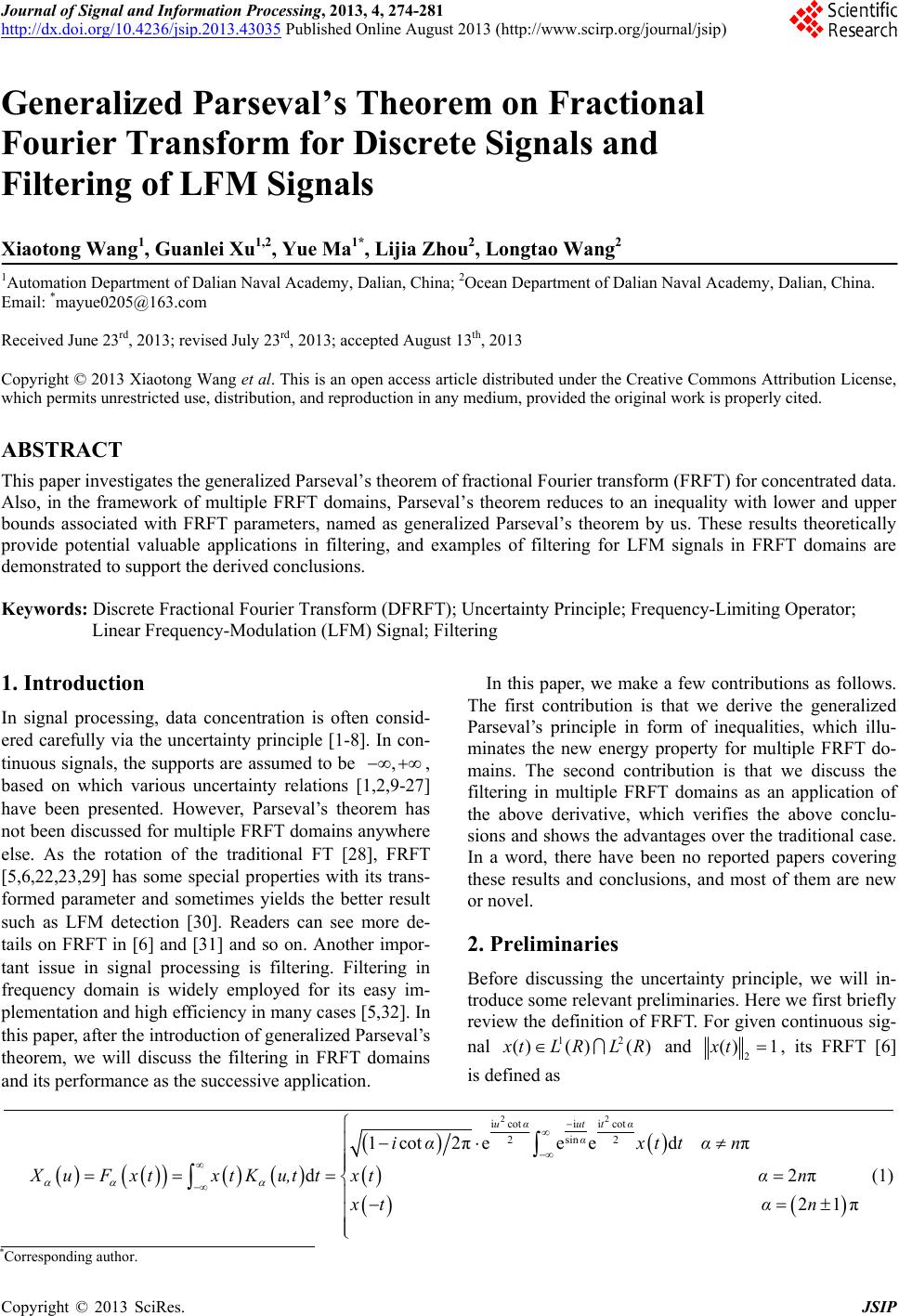
|