Journal of Modern Physics, 2013, 4, 1119-1122
http://dx.doi.org/10.4236/jmp.2013.48150 Published Online August 2013 (http://www.scirp.org/journal/jmp)
Erratum: The Gravitational Radiation Emitted by a
System Consisting of a Point Particle in Close Orbit
around a Schwarzschild Black Hole
Amos S. Kubeka
Department of Mathematical Sciences, University of South Africa, Pretoria, South Africa
Email: kubekas@unisa.ac.za
Received January 8, 2013; revised March 4, 2013; accepted May 26, 2013
Copyright © 2013 Amos S. Kubeka. This is an open access article distributed under the Creative Commons Attribution License,
which permits unrestricted use, distribution, and reproduction in any medium, provided the original work is properly cited.
ABSTRACT
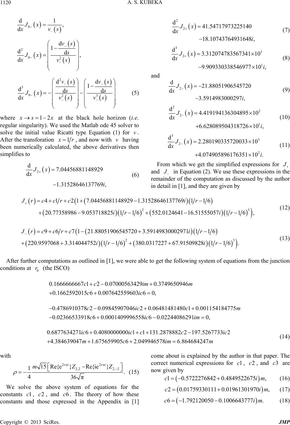
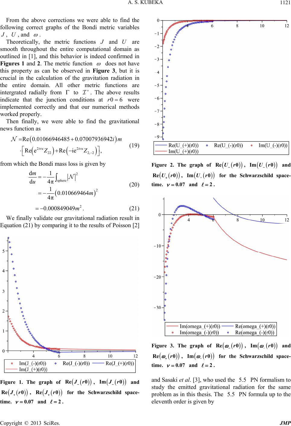
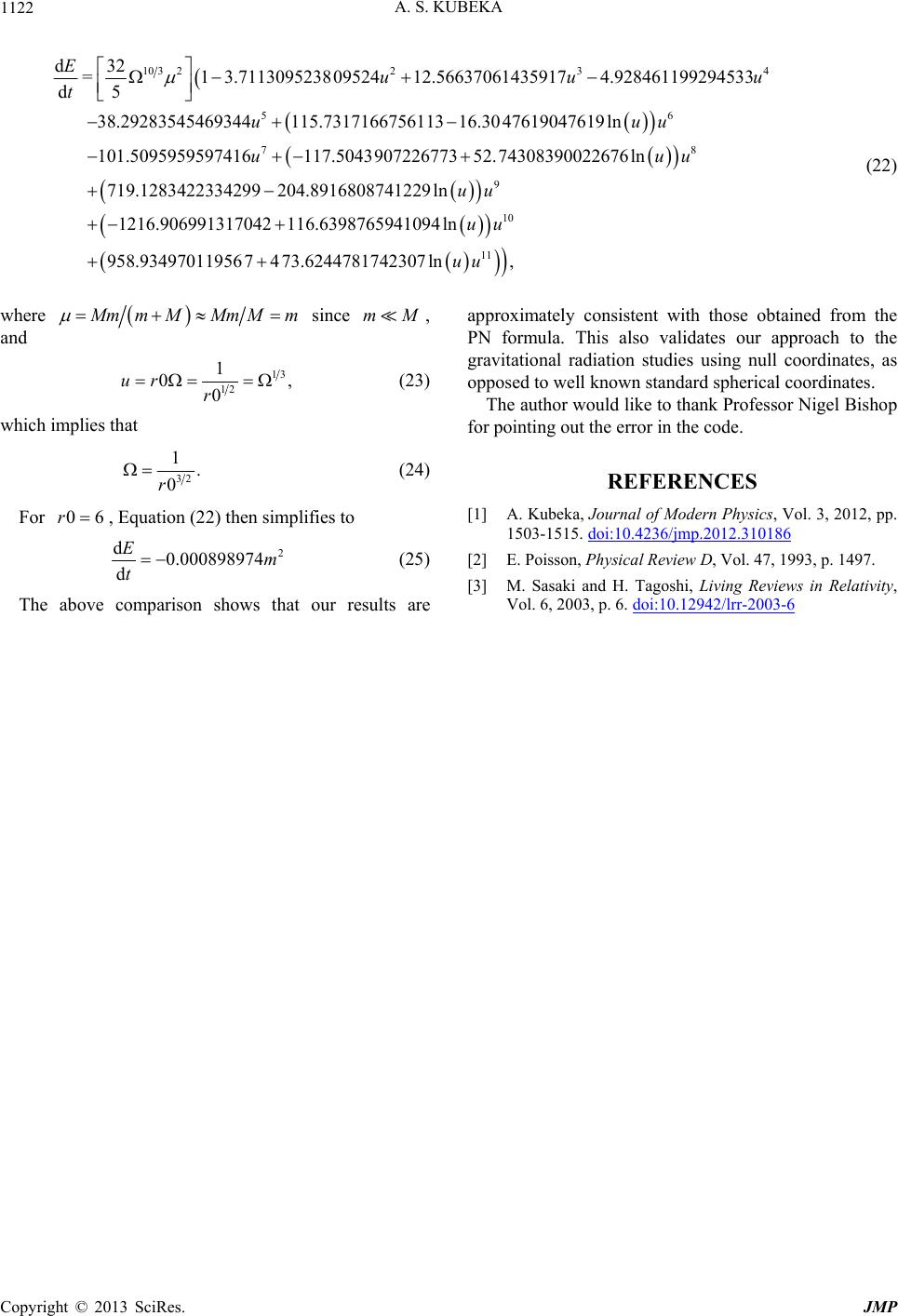
We correct from the previous paper: the first, second and third order derivatives of the Bondi metric function J at the
ISCO of the binary system consisting of a Schwarzschild black hole and a point particle. Previously, these derivatives
where not correctly determined and that resulted in the incorrect determination of the emitted gravitational radiation at
null infinity. The now correctly calculated gravitational radiation is now in full agreement with that obtained by the
standard 5.5 PN formalism to about ninety eight percent. The small percentage difference observed is due to the slow
convergence property of the PN formalism as compared to the null cone formalism, otherwise the results are basically
the same.
Keywords: Black Hole; Particle; Gravitational Radiation; Null Infinity
1. Errors
1) Equation (13) in [1] should be correctly read as


2
d2
=127 8
d12
vv i
x
vxx
xx
xx





v
(1)
where
is the orbital frequency of the system.
2) Also in the original paper by the author [1], there
was an inherent numerical error due to the incorrect
determination of the first, second, and third order
derivatives of the Bondi metric function
0
J
x
and
0
J
x
in
 
0
0
41 2
96 7.
J
xccxcJx
J
xccxcJx

 
 
(2)
The correct derivatives are now here given by
 

0
d,
d
s
vs
Jx
xsvs








2
2
0
d
dd,
d
vs svs
s
Jx
xsvssvs





 




(3)

  











2
2
3
02
2
dd dd
dd
ddd
2
d
,
vs vsvs vs
vs
ss
svs ss
Jx
xsvssv s
svs svs
sv ssv s
 
 



 






 
















svssvs
(4)
and
C
opyright © 2013 SciRes. JMP
A. S. KUBEKA
1120
 
0
d1
,
dJx
x
vs



2
02
d
1
dd,
d
vs
s
Jx
xvs











2
3
023
dd
1
dd
d
vs vs
s
Jx
xvsv







 






ds
s
(5)
where 12
sx at the black hole horizon (i.e.
regular singularity). We used the Matlab ode 45 solver to
solve the initial value Ricatti type Equation (1) for .
After the transforation
v
1
x
r, and now with having
been numerically calculated, the above derivatives then
simplifies to
v

2
d7.04456881148929
d
1.31528646137769 ,
Jx
x
i
(6)

2
2
d41.54717973225140
d
18.10743764931648 ,
Jx
xi
(7)

3
3
2
1
d3.312074783567341 10
d
9.90933033854697710 ,
Jx
x
i


(8)
and

2
d21.88051906545720
d
3.5914983000297 ,
Jx
xi

(9)

2
2
2
1
d4.419194136304895 10
d
6.62808950431872610 ,
Jx
x
i


(10)

3
3
2
2
d2.280190335720033 10
d
4.074905896176351 10.
Jx
x
i


(11)
From which we get the simplified expressions for
J
and
J
in Equation (2). We use these expressions in the
remainder of the computation as discussed by the author
in detail in [1], and they are given by



 
23
41217.044568811489291.3152864613776911 6
20.773589869.0537188251 16552.012464116.515550571 16,
Jr c crcir
ir ir
 

(12)
 
23
967121.880519065457203.5914983000297111 6
220.95970683.31404475211 6380.031722767.9150982811 6.
Jr c crcir
ir ir
 
  
(13)
After further computations as outlined in [1], we were able to get the following system of equations from the junction
conditions at (the ISCO)
0
r
0.1666666667 120.070005634290.3749650946
0.1662592015 60.00764255960360,
ccim m
cic
 

0.478691037820.0984590704620.06481481480 10.001154184775
0.02366533918 60.000140999655860.022440862910,
cicc
cicim


m
0.687763427160.408000000011131.2878882 2197.52677332
4.3846390471.675659905 62.0499465786.864684247
icic ccic
mcim m

  (14)
with
22
2,22, 2
15 Re{e}Re{ie}
1.
436 π
ui ui
mZ


 Z
(15)
We solve the above system of equations for the
constants , , and . The theory of how these
constants and those expressed in the Appendix in [1]
come about is explained by the author in that paper. The
correct numerical expressions for , , and are
now given by
1c2c6c
1c2c3c
10.5722276842 0.484, 9522675cim
(16)
20.01759330111 0.01,ci m961301970 (17)
61.792120050 0.1006643777.ci m
(18)
Copyright © 2013 SciRes. JMP
A. S. KUBEKA 1121
From the above corrections we were able to find the
following correct graphs of the Bondi metric variables
J
, , and U
.
Theoretically, the metric functions
J
and are
smooth throughout the entire computational domain as
outlined in [1], and this behavior is indeed confirmed in
Figures 1 and 2. The metric function
U
does not have
this property as can be observed in Figure 3, but it is
crucial in the calculation of the gravitation radiation in
the entire domain. All other metric functions are
intergrated radially from to . The above results
indicate that the junction conditions at
0r6
were
implemented correctly and that our numerical methods
worked properly.
Then finally, we were able to find the gravitational
news function as

 
22
222,2
Re 0.010669464850.07007936942
Re eReie,
iu iu
im
ZZ





(19)
from which the Bondi mass loss is given by

2
sphere
2
d1
d4π
10.010669464
4π
m
u
m


(20)
2
0.000849049 m . (21)
We finally validate our gravitational radiation result in
Equation (21) by comparing it to the results of Poisson [2]
Figure 1. The graph of
Re 0
J
r
,
Im 0
J
r
and
Re 0
J
r
,
Re 0
J
r
for the Schwarzschild space-
time. 0.07
and .
2
Figure 2. The graph of ,


Re 0Ur
Im 0Ur
and
Re 0Ur
,
Im 0Ur for the Schwarzschild space-
time. 0.07
and 2
.
Figure 3. The graph of ,


Re 0r
Im 0r
and
Re 0r
,
Im 0r
for the Schwarzschild space-
time. 0.07
and 2
.
and Sasaki et al. [3], who used the PN formalism to
study the emitted gravitational radiation for the same
problem as in this thesis. The PN formula up to the
leventh order is given by
5.5
5.5
e
Copyright © 2013 SciRes. JMP
A. S. KUBEKA
Copyright © 2013 SciRes. JMP
1122

10 32234
5 6
7
d32
=1 3.71130952380952412.566370614359174.928461199294533
d5
38.29283545469344115.731716675611316.30 47619047619 ln
101.5095959597416117.5043907226773 52.74308390022676ln
Euu
t
uu
u












8
9
10
11
719.1283422334299204.8916808741229 ln
1216.906991317042116.6398765941094 ln
958.93497011956 74 73.6244781742307 ln,
uu
uu
uu
uu

 

u
u
(22)
where

M
mmMMmM m

since ,
and
mM
13
12
1
0
0
ur r
 ,
(23)
which implies that
32
1.
0r
 (24)
For , Equation (22) then simplifies to
06r
2
d0.000898974
d
Em
t (25)
The above comparison shows that our results are
approximately consistent with those obtained from the
PN formula. This also validates our approach to the
gravitational radiation studies using null coordinates, as
opposed to well known standard spherical coordinates.
The author would like to thank Professor Nigel Bishop
for pointing out the error in the code.
REFERENCES
[1] A. Kubeka, Journal of Modern Physics, Vol. 3, 2012, pp.
1503-1515. doi:10.4236/jmp.2012.310186
[2] E. Poisson, Physical Review D, Vol. 47, 1993, p. 1497.
[3] M. Sasaki and H. Tagoshi, Living Reviews in Relativity,
Vol. 6, 2003, p. 6. doi:10.12942/lrr-2003-6