Paper Menu >>
Journal Menu >>
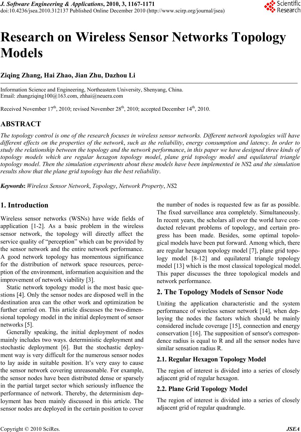 J. Software Engineering & Applications, 2010, 3, 1167-1171 doi:10.4236/jsea.2010.312137 Published Online December 2010 (http://www.scirp.org/journal/jsea) Copyright © 2010 SciRes. JSEA Research on Wireless Sensor Networks Topology Models Ziqing Zhang, Hai Zhao, Jian Zhu, Dazhou Li Information Science and En g i ne e ri n g , Northeastern University, Shenyang, China. Email: zhangziqing100@163.com, zhhai@neuera.com Received November 17th, 2010; revised November 28th, 2010; accepted December 14th, 2010. ABSTRACT The topology con trol is one of the research focuses in wireless sensor networks. Different netwo rk topologies will have different effects on the properties of the network, such as the reliability, energy consumption and latency. In order to study the relationship between the topology and the network performance, in this paper we have designed three kinds of topology models which are regular hexagon topology model, plane grid topology model and equilateral triangle topology model. Then the simulation experiments about these models have been implemented in NS2 and the simulation results show that the plane grid topology has the best reliability. Keywords: Wireless Sensor Network, Topology, Network Property, NS2 1. Introduction Wireless sensor networks (WSNs) have wide fields of application [1-2]. As a basic problem in the wireless sensor network, the topology will directly affect the service quality of “percep tion” which can be provided by the sensor network and the entire network performance. A good network topology has momentous significance for the distribution of network space resources, perce- ption of the environment, information acquisition and the improvement of network viability [3]. Static network topology model is the most basic que- stions [4]. Only the sensor nodes are disposed well in the destination area can the other work and optimization be further carried on. This article discusses the two-dimen- sional topology mode l in the initial deplo yment of sensor networks [5] . Generally speaking, the initial deployment of nodes mainly includes two ways. deterministic deplo yment and stochastic deployment [6]. But the stochastic deploy- ment way is very difficult for the numerous sensor nodes to lay aside in suitable position. It’s very easy to cause the sensor network covering unreasonable. For example, the sensor nodes have been distributed dense or sparsely in the partial target sector which seriously influence the performance of network. Thereby, the determinism dep- loyment has been mainly discussed in this article. The sensor nodes are deployed in the certain position to cover the number of nodes is requested few as far as possible. The fixed surveillance area completely. Simultaneously. In recent years, the scholars all over the world have con- ducted relevant problems of topology, and certain pro- gress has been made. Besides, some optimal topolo- gical models have been put forward. Among which, there are regular hexagon topology model [7], plane grid topo- logy model [8-12] and equilateral triangle topology model [13] which is the most classical topological model. This paper discusses the three topological models and network perfor mance. 2. The Topology Models of Sensor Node Uniting the application characteristic and the system performance of wireless sensor network [14], when dep- loying the nodes the factors which should be mainly considered include coverage [15], connection and energy conservation [16 ]. The supposition of sensor's correspon- dence radius is equal to R and all the sensor nodes have similar sensation radius R. 2.1. Regular Hexagon Topology Model The region of interest is divided into a series of closely adjacent grid o f reg ul a r he xagon. 2.2. Plane Grid Topology Model The region of interest is divided into a series of closely adjacent grid of regular quadrangle. 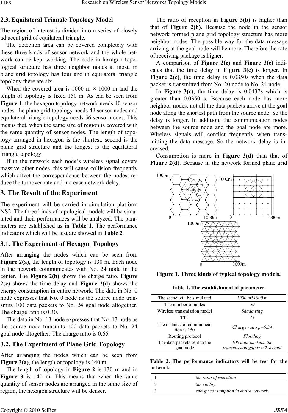 Research on Wireless Sensor Networks Topology Models Copyright © 2010 SciRes. JSEA 1168 2.3. Equilateral Triangle Topology Model The region of interest is divided into a series of closely adjacent grid of equilateral triangle. The detection area can be covered completely with these three kinds of sensor network and the whole net- work can be kept working. The node in hexagon topo- logical structure has three neighbor nodes at most, in plane grid topology has four and in equilateral triangle topology there are six. When the covered area is 1000 m × 1000 m and the length of topology is fixed 150 m. As can be seen from Figure 1, the hexagon topolog y network n eeds 40 sensor nodes, the plane grid topology needs 49 sensor nodes and equilateral triangle topolog y needs 56 sensor nodes. This means that, when the same size of region is covered with the same quantity of sensor nodes. The length of topo- logy arranged in hexagon is the shortest, second is the plane grid structure and the longest is the equilateral triangle topology. If in the network each node’s wireless signal covers massive other nodes, this will cause collision frequently which affect the correspondence between the nodes, re- duce the turnover rate and increase network delay. 3. The Result of the Experiment The experiment will be carried in simulation platform NS2. The three kinds of topological models will be simu- lated and their performances will be analyzed. The para- meters are established as in Table 1. The performance indicators which will be test are showed in Table 2. 3.1. The Experiment of Hexagon Topology After arranging the nodes which can be seen from Figure 2(a), the length of topology is 130 m. Each node in the network communicates with No. 24 node in the center. The Figure 2(b) shows the charge ratio, Figure 2(c) shows the time delay and Figure 2(d) shows the energy consumption in entire network. The data in No. 0 node expresses that No. 0 node as the source node tran- smits 100 data packets to No. 24 goal node altogether. The charge ratio is 0.30. The data in No. 13 node expresses that No. 13 node as the source node transmits 100 data packets to No. 24 goal node altogether. The charge ratio is 0.65. 3.2. The Experiment of Plane Grid Topology After arranging the nodes which can be seen from Figure 3(a), the length of topology is 140 m. The length of topology in Figure 2 is 130 m and in Figure 3 is 140 m. This means that when the same quantity of sensor nod es are arranged in the same size of region, the hexagon structure will be denser. The ratio of reception in Figure 3(b) is higher than that of Figure 2(b). Because the node in the sensor network formed plane grid topology structure has more neighbor nodes. The possible way for the data message arriving at the goal node will be more. Therefore the rate of receiving package is higher. A comparison of Figure 2(c) and Figure 3(c) indi- cates that the time delay in Figure 3(c) is longer. In Figure 2(c), the time delay is 0.0350s when the data packet is transmitted from No. 20 node to No. 24 node. In Figure 3(c), the time delay is 0.0437s which is greater than 0.0350 s. Because each node has more neighbor nodes, not all the data packets arrive at the goal node along the shortest path from the source node. So the delay is longer. In addition, the communication nodes between the source node and the goal node are more. Wireless signals will conflict frequently when trans- mitting the data message. So the network delay is in- creased. Consumption is more in Figure 3(d) than that of Figure 2(d). Because in the network formed plane grid Figure 1. Three kinds of typical topology mo dels. Table 1. The establishment of parameter. The scene will be simulated 1000 m*1000 m The number of nodes 50 Wireless transmission model Shadowing TTL 13 The distance of communica- tion is 150 Charge ratio p=0.34 Routing protocol Flooding The data packets sent to the goal node 100 data packets, the transmission gap is 0.2 second Table 2. The performance indicators will be test for the network. 1the ratio o f r ece p tion 2 t ime dela y 3energy consumption in entire networ k 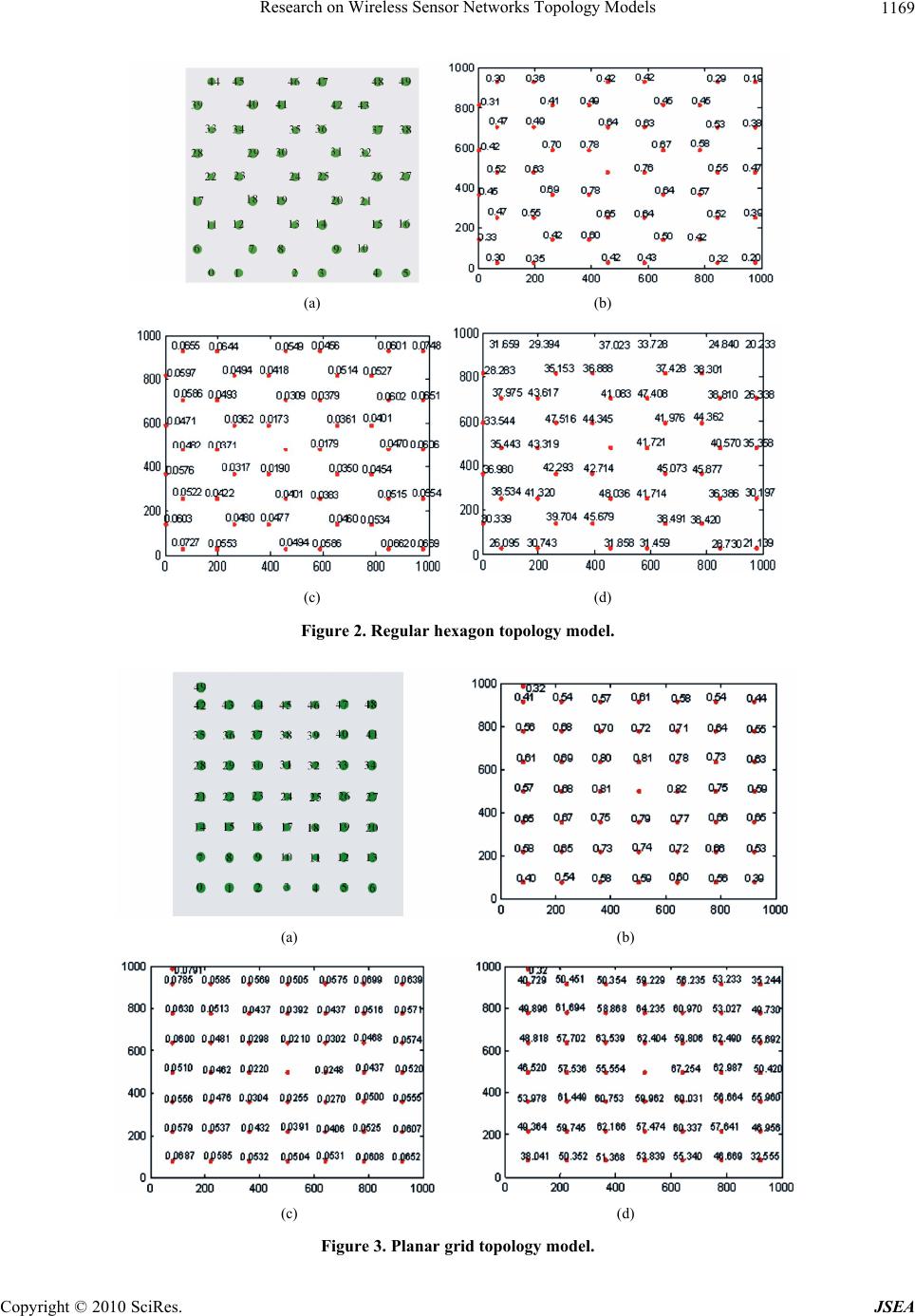 Research on Wireless Sensor Networks Topology Models Copyright © 2010 SciRes. JSEA 1169 (a) (b) (c) (d) Figure 2. Regular hexagon topology model. (a) (b) (c) (d) Figure 3. Planar grid topology model. 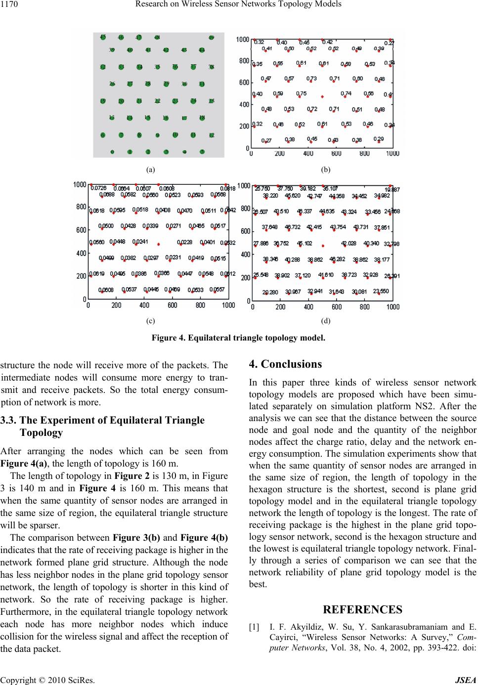 Research on Wireless Sensor Networks Topology Models Copyright © 2010 SciRes. JSEA 1170 (a) (b) (c) (d) Figure 4. Equilateral triangle topology model. structure the node will receive more of the packets. The intermediate nodes will consume more energy to tran- smit and receive packets. So the total energy consum- ption of network is more . 3.3. The Experiment of Equilateral Triangle Topology After arranging the nodes which can be seen from Figure 4(a), the length of topology is 160 m. The length of topology in Figure 2 is 130 m, in Figure 3 is 140 m and in Figure 4 is 160 m. This means that when the same quantity of sensor nodes are arranged in the same size of region, the equilateral triangle structure will be sparser. The comparison between Figure 3(b) and Figure 4(b) indicates that the rate of receiving package is higher in the network formed plane grid structure. Although the node has less neighbor nodes in the plane grid topology sensor network, the length of topology is shorter in this kind of network. So the rate of receiving package is higher. Furthermore, in the equilateral triangle topology network each node has more neighbor nodes which induce collision for the wireless signal and affect the reception of the data packet. 4. Conclusions In this paper three kinds of wireless sensor network topology models are proposed which have been simu- lated separately on simulation platform NS2. After the analysis we can see that the distance between the source node and goal node and the quantity of the neighbor nodes affect the charge ratio, delay and the network en- ergy consumption. The simulation experiments show that when the same quantity of sensor nodes are arranged in the same size of region, the length of topology in the hexagon structure is the shortest, second is plane grid topology model and in the equilateral triangle topology network the length of topology is the longest. The rate of receiving package is the highest in the plane grid topo- logy sensor netw ork, second is the hexagon structur e and the lowest is equilateral triangle topology netw ork. Final- ly through a series of comparison we can see that the network reliability of plane grid topology model is the best. REFERENCES [1] I. F. Akyildiz, W. Su, Y. Sankarasubramaniam and E. Cayirci, “Wireless Sensor Networks: A Survey,” Com- puter Networks, Vol. 38, No. 4, 2002, pp. 393-422. doi:  Research on Wireless Sensor Networks Topology Models Copyright © 2010 SciRes. JSEA 1171 10.1016/S1389-1286(01)00302-4 [2] S. Tilak, N. B. Abu-Ghazaleh and W. Heinzelman, “A Taxonomy of Wireless Microsensor Network Models," ACM Mobile Computing and Communications Review, Vol. 6 No. 2, 2002, pp. 28-36. doi:10.1145/565702. 565708 [3] C. F. Huang and Y. C. Tseng, “The Coverage Problem in a Wireless Sensor Network,” Proceedings of ACM WSNA, San Diego, 19 September 2003, pp.519-528 doi:10.1145/ 941350.941367 [4] C. Shen, C. Srisathapornphat and C. Jaikaeo, “Sensor Information Networking Architecture and Applications,” IEEE Personal. Communication, Vol. 8, No. 4, 2001, pp. 52-59. doi:10.1109/98.944004. [5] S. H. Yang, M. L. Li, and J. Wu, “Scan-Based Move- ment-Assisted Sensor DePloyment Methodin Wireless Sensor Networks,” IEEE Transactions on Parallel and Distributed Systems, Vol. 18, No. 8, 2007, pp.1108-1121. doi:10.1109/TPDS.2007.1048 [6] A. Salhieh, J. Weinmann, M. Kochhal and L. Schwiebert, “Power Efficient Topologies for Wireless Sensor Net- works,” International Conference on Parallel Processing, Valencia, 3-7 Sepmber 2001, pp. 156-163. [7] K. Chakrabarty, S. S. Iyengar, H. R. Qi and E. C. Cho., “Grid Coverage for Surveillance and Target Location in Distributed Sensor Networks,” IEEE Transactions on Computers. Vol. 51, No. 12, 2002, pp. 1448-1453. doi: 10.1109/TC.2002.1146711 [8] Q. S. Wu, N. S. V. Rao and X. J. Du, et al., “On Efficient Deployment of Sensors on Planar Grid,” IEEE Computer Communications. Vol. 30, No. 14-15, 2007, pp. 2721-2734. doi:10.1016/j.comcom.2007.05.012 [9] K. Chakrabarty, S. S. Iyengar, H. R. Qi and E. Cho, “Grid Coverage for Surveillance and Target Location in Distributed Sensor Networks,” IEEE Transactions on Computers, Vol. 51, No. 12, 2002, pp. 1448-1453. doi: 10.1109/TC.2002.1146711 [10] S. Shakkottai, R. Srikant and N. Shroff. “Unreliable Sensor Grids: Coverage, Connectivity and Diameter.” IEEE Press, San Francisco, 2003. [11] C.-H. Wu, K.-C. Lee and Y.-C. Chung, “A Delaunay Triangulation Based Method for Wireless Sensor Net- work Deployment,” IEEE Computer Communications, Vol. 30, No. 14-15, 2007, pp. 2744-2752. doi:10.1016 /j.comcom.2007.05.017 [12] J. L. Hill, “System Architecture for Wireless Sensor Networks,” Ph.D. Thesis, Computer Science University of California , Berkeley, 2003. [13] Q. Jiang, D. Manivannan, “Routing protocols for sensor networks,” Consumer Communications and Networking Conference, Las Vegas, 5-8 January 2004, pp. 93-98. [14] S. S. Dhillon and K. Chakrabarty, “Sensor Placement for Effective Coverage and Surveillance in Distributed Sen- sor Networks,” IEEE Wireless Communications and Networking Conference, New Orleans, 20-20 March 2003, pp. 1609-1614. [15] S. Meguerdichian, F. Koushanfar, M. Potkonjak and M. Srivastava, “Coverage Problems in Wireless Ad Hoc sensor Networks,” Proceedings of IEEE Infocom, Alaska, 22-26 April 2001, pp. 22-26. [16] Y. C. Wang, C. C. Hu and Y. C. Tseng, “Efficient De- ployment Algorithms for Ensuring Coverage and Con- nectivity of Wireless Sensor Networks,” Wireless Internet Conference, Budapest, 10-14 July 2005, pp. 114-121. doi:10.1109/WICON.2005.13 |