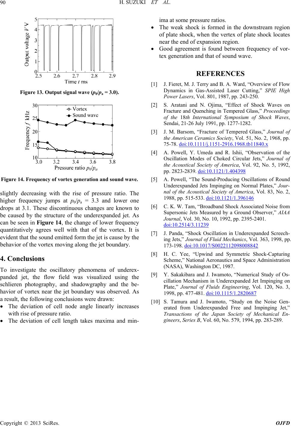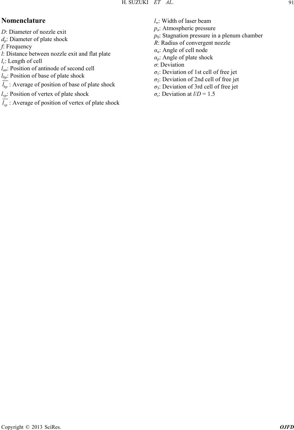
H. SUZUKI ET AL.
86
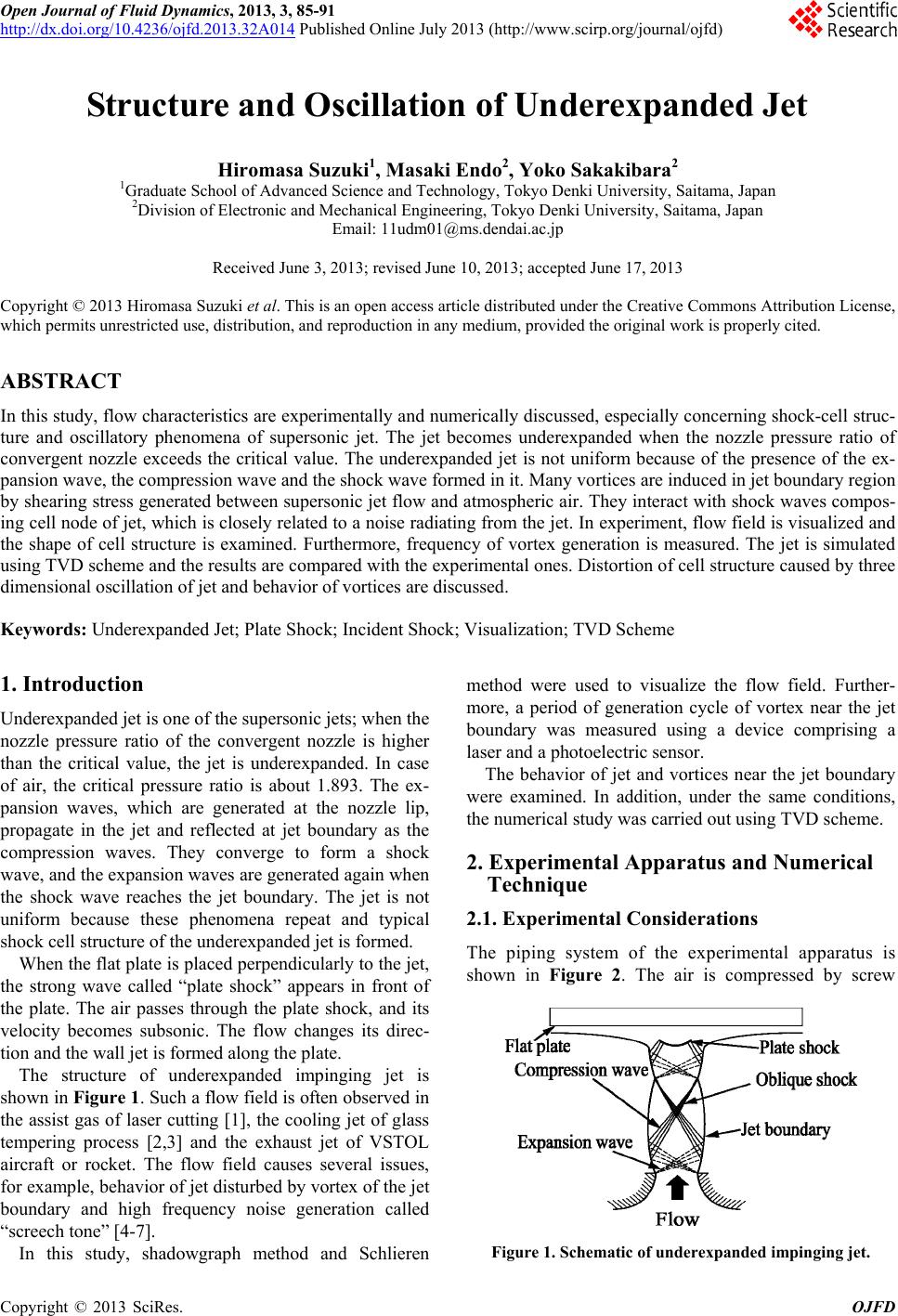
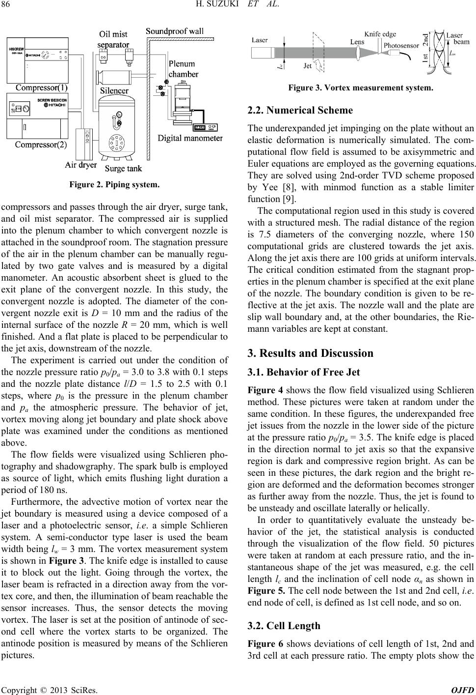
Figure 2. Piping system.
compressors and passes through the air dryer, surge tank,
and oil mist separator. The compressed air is supplied
into the plenum chamber to which convergent nozzle is
attached in the soundproof room. The stagnation pr essure
of the air in the plenum chamber can be manually regu-
lated by two gate valves and is measured by a digital
manometer. An acoustic absorbent sheet is glued to the
exit plane of the convergent nozzle. In this study, the
convergent nozzle is adopted. The diameter of the con-
vergent nozzle exit is D = 10 mm and the radius of the
internal surface of the nozzle R = 20 mm, which is well
finished. And a flat plate is placed to be perpendicular to
the jet axis, downstream of the nozzle.
The experiment is carried out under the condition of
the nozzle pressure ratio p0/pa = 3.0 to 3.8 with 0.1 steps
and the nozzle plate distance l/D = 1.5 to 2.5 with 0.1
steps, where p0 is the pressure in the plenum chamber
and pa the atmospheric pressure. The behavior of jet,
vortex moving along j et boundary and plate shock above
plate was examined under the conditions as mentioned
above.
The flow fields were visualized using Schlieren pho-
tography and shadowgraphy. The spark bulb is employed
as source of light, which emits flushing light duration a
period of 18 0 n s .
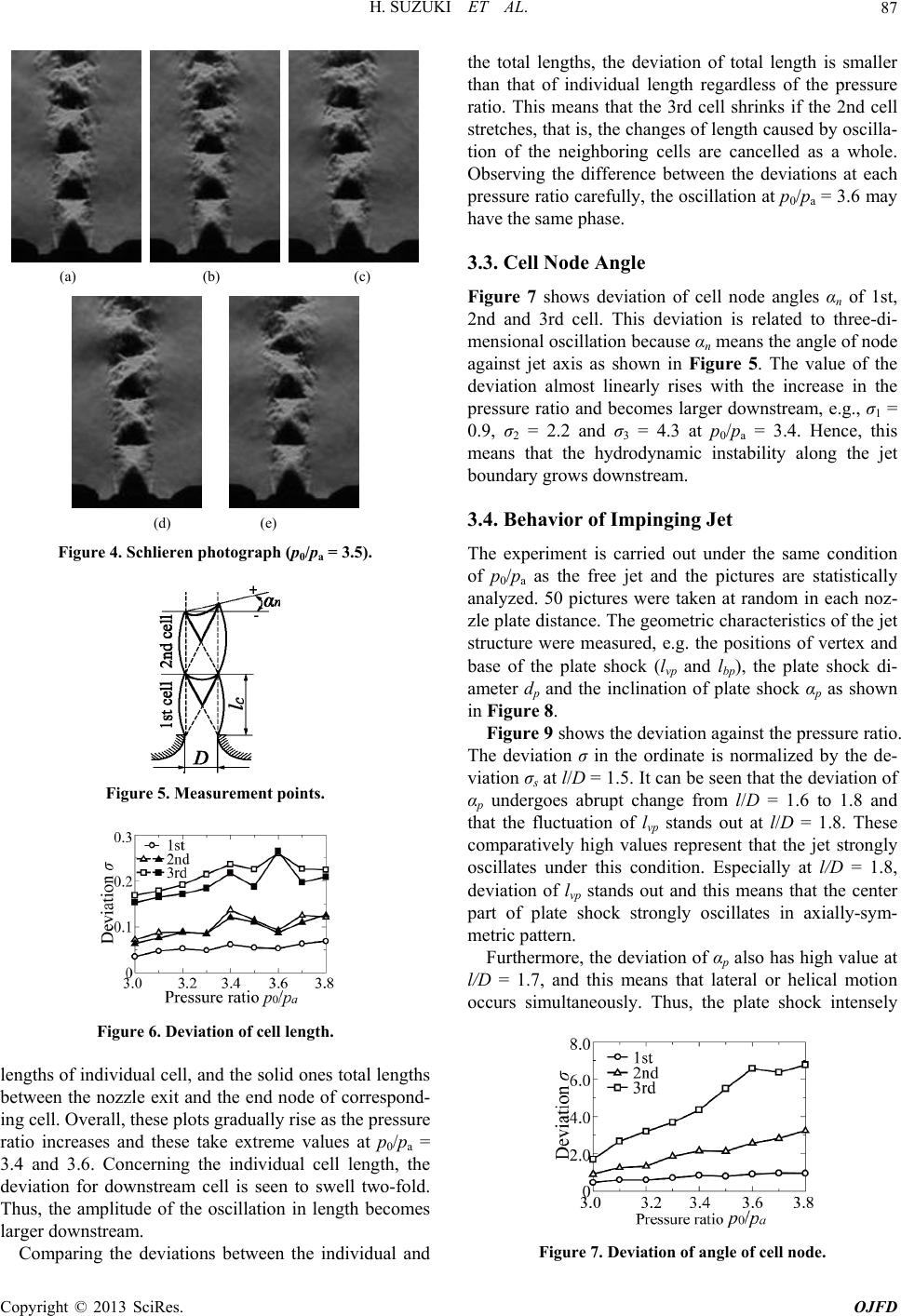
Furthermore, the advective motion of vortex near the
jet boundary is measured using a device composed of a
laser and a photoelectric sensor, i.e. a simple Schlieren
system. A semi-conductor type laser is used the beam
width being lw = 3 mm. The vortex measurement system
is shown in Figure 3. The knife edge is installed to cause
it to block out the light. Going through the vortex, the
laser beam is refracted in a direction away from the vor-
tex core, and then, the illumination of beam reachable the
sensor increases. Thus, the sensor detects the moving
vortex. The laser is set at the position of antinode of sec-
ond cell where the vortex starts to be organized. The
antinode position is measured by means of the Schlieren
pictures.
Figure 3. Vortex measurement system.
2.2. Numerical Scheme
The underexpanded jet impinging on the plate without an
elastic deformation is numerically simulated. The com-
putational flow field is assumed to be axisymmetric and
Euler equations are employed as the governing equations.
They are solved using 2nd-order TVD scheme proposed
by Yee [8], with minmod function as a stable limiter
function [9].
The computational region used in this study is covered
with a structured mesh. The radial distance of the region
is 7.5 diameters of the converging nozzle, where 150
computational grids are clustered towards the jet axis.
Along the jet axis there are 100 grids at uniform intervals.
The critical condition estimated from the stagnant prop-
erties in the plenum chamber is specified at the exit plane
of the nozzle. The boundary condition is given to be re-
flective at the jet axis. The nozzle wall and the plate are
slip wall boundary and, at the other boundaries, the Rie-
mann variables are kept at constant.
3. Results and Discussion
3.1. Behavior of Free Jet
Figure 4 shows the flow field visualized using Sch lieren
method. These pictures were taken at random under the
same condition. In these figures, the underexpanded free
jet issues from the nozzle in the lower side of the picture
at the pressure ratio p0/pa = 3.5. The knife edge is placed
in the direction normal to jet axis so that the expansive
region is dark and compressive region bright. As can be
seen in these pictures, the dark region and the bright re-
gion are deformed and the deformation becomes stronger
as further away from the nozzle. Thus, the jet is found to
be unsteady and oscillate laterally or helically.
In order to quantitatively evaluate the unsteady be-
havior of the jet, the statistical analysis is conducted
through the visualization of the flow field. 50 pictures
were taken at random at each pressure ratio, and the in-
stantaneous shape of the jet was measured, e.g. the cell
length lc and the inclination of cell node αn as shown in
Figure 5. The cell node between the 1st and 2nd cell, i.e.
end node of cell, is defined as 1st cell node, and so on.
3.2. Cell Length
Figure 6 shows deviations of cell length of 1st, 2nd and
3rd cell at each pressure ratio. The empty plots show the
Copyright © 2013 SciRes. OJFD