Optics and Photonics Journal, 2013, 3, 322-330
doi:10.4236/opj.2013.32B075 Published Online June 2013 (http://www.scirp.org/journal/opj)
Novel Understanding of Electron States Architecture
and Its Dimensionality in Semiconductors
Xiaomin Ren
State Key Laboratory of Information Photonics and Optical Communications
(Beijing University of Posts and Telecommunications), and Zh. I. Alferov Russian-Chinese Joint
Laboratory of Information Optoelectronics and Nanoheterostructures, Beijing, China
Received February 27, 2013; revised March 27, 2013; accepted May 8, 2013
ABSTRACT
So me important insights into the electron-states-arc hitecture (ESA) and its dimensionality (from 3 to 0) in a semicon-
ductor (or generally crystalline) material are obtained. The s elf -co ns is te ncy o f t he se t o f de nsit y of st a te s ( DO S ) e xp re s-
sions with different dimensionalities is remediated through the clarification and rearrangement of the wave-function
boundary conditions for working o ut the eigenvalues in the wave vector space. The actually too roughly observed and
theoreticall y unpredicted c ritical points for the d imensionalit y transitions referring to the i ntege r ones are revealed upon
an un usual as sumptio n of the intri nsic ener gy-level dispersion (ELD). The ELD based quantitative physical model had
been established o n an immediate instinct at the very beginning and has been properly modified afterwards. The uncer-
tainty regarding the relationship between the de Broglie wavelength of electrons and the dimensionality transitions ,
seeming somewhat mysterious before, is consequentially eliminated. The effect of the material dimensions on the E LD
width is also predicted and has b ee n i ncl ude d in the mod e l. T he co nti nuo us evo lu ti on o f t he ES A dimensionalit y is con-
vincingly and comprehensively interpreted and t hus the area of the fractional ESA dimensionalities is opened. Another
new assumption of the spatial extension shrinkage (SES) closely related to the ELD has also been made and thus the
understanding of the behavior of an electron or, in a general sense, a particle has become more comprehensive. This
work would manifest itself a new basis for further development of nanoheterostructures (or low dimensional hetero-
structures including the quantum wells, quantum wires, quantum dots and especially the hetero-dime nsio nal str uct ures) .
Expected should also be the possible inventions of some novel electronic and optoelectronic devices. More basically, it
leads to a new quantum mechanical picture, the essential modifications of Schrödinger equation and Newtonian equa-
tion that give rise to a full cosmic-scope picture, and a super-low-speed relativity assumption.
Keywords: Energy-level Dispe r sion; Spatial E xtension Shrinkage; E lec tr o n -s tate s-architecture; Density o f States; Di-
mensionality; Quantum Wells, Wires and Dots; Schrödinger Equation; Newtonian Equation; Relativity
1. Introduction
Both the classical and the nano- heterostructures of semi-
conductors have developed dramatically based on the
well-recognized theories, especially the theory on the
density of states (DOS) of electrons in a semiconductor
(or generally crystalline) material and the relevant elec-
tron-states-architecture (ESA) dimensionality [1]. However,
some problems exist in the previous theory and it had
been suspected that some fundamental theoretical
changes would be needed for the improvement. Both
unus ual ass u mptio ns of the energy-level dispersion (ELD)
[2-3] and the spatial extension shrinkage (SES) have
been proposed and it is shown that they have acted quite
well for the improvement. And, in proceeding with this
investigation, the quantum mechanical picture and the
relevant fundamental theorie s have really been changed.
2. Important Insights into the Previous
Theory and a Summary of the Problems
In this paper, without the loss of generality, the investi-
gations on the ESA and its dimensionality will be re-
stricted only on the case of a conduction band (or a band
with a l owest minimu m). The DOS expr essions given b y
the previous theory in this case for a bulk material (3D),
a quantum well (2D), a quantum wire (1D) and a quan-
tum dot (0D) are as follo ws, respectively:
( )
3
2
23
()2( -)
nc
c
m EE
E
ρπ
∗
=

(1)
( )
( )
2
,
n
c zcn
nz
m
ELE E
L
ρπ
∗
= Θ−
∑

(2)
where

X. M. REN
323
2
2, =1, 2, 3,
2
cn cz
n
n
EE n
L m
π
∗

= +±±±


…
( )
( )
,
,,
,, 2
nc mn
cyz mn yzc mn
m EE
EL LLLE E ρπ
∗Θ−
=−
∑

(3)
where,
22
2
,
+
2
c mncyz
n
mn
EE LL
m
ππ
∗




= +







,
, =1, 2, 3, mn ±±±…
( ) ( )
,
,,
2
,,,
cxyzc lmn
lmn xyz
EL L LEE
LLL
ρδ = −
∑
(4)
where,
2
22
2
,
++,
2
c lmncxyz
n
lmn
EE LLL
m
π ππ
∗


 

= +
 


 


,, =1, 2, 3, lmn±±±…
It is noted that all the material structures under the in-
vestigations here are assumed of the cuboidal shapes.
The material sizes in the three directions are denoted by
Lx, Ly, and Lz, respectively. In addition, the symbols
E
,
c
E
and
n
m
∗
are the electron energy with an arbitrary
value, the electron energy at the bottom of the conduc-
tion band (or at the minimum of a specified band) and the
effective mass of an electron in the band, respectively;
2
h
π
=
is a quantity related uniquely to the Planck
constant h; and,
( )
10
00
x
x
x≥
<
Θ={ is a Heaviside function.
Altho ugh al most e very one o f us is quite fami liar with
these e xpressions, it is st ill necessary for us to ga in so me
essential insights into them:
1) In a rigorous sense, Eq. (1), the so-called “3D ex-
pression”, is true only when Lx, Ly, and Lz are all infi-
nitely long. Otherwise, the value of the
k

-space volume
occupied by a single state cannot be identical everywhere
and the derivation of this equation cannot be rigorously
valid. So, at the most, it could be applicable only ap-
proximately to the case of a large enough material vo-
lume.
2) Attention should also be paid to another issue re-
garding the derivation of Eq. (1). In the de r ivation, the
number of states per unit k

-space volume is actually (or
should be) taken as
*
,,
3
33
,,
1
=2lim 222
lim
44
j
j
L
j xyz
xyz
xyz
L
j xyz
dZ
d
LLL
LLL
πππ
ππ
→∞
=
→∞
=
×
Ω
 

 




∞
= =
(5)
where, the intervals between the adjacent wave-vector
eigenvalues corresponding to the specified pairs of the
wave-function solutions are taken as
2
lim
x
Lx
L
π
→∞
，
2
lim
y
Ly
L
π
→∞
and 2 lim
z
Lz
L
π
→∞ in the three directions, kx, ky, and kz, re-
spectively, b y adop ting the periodic boundary conditions.
This kind of conditions are truly valid upon a homogen-
ous-material assumption which means that the materials
within and outside the volume defined by Lx, Ly, and Lz
are exactly the same. This is an absolutely-homogenous
ideal (infinite ) 3D model and thus, in p rinci ple, the use of
Eq. (1) should be excluded from the modeling o f a hete-
rostruct ure syst em.
For the complete ness of de scriptio n, it should be stated
here additionally that, based on this ideal 3D model with
the homogenous-material assumption, Eq. (1) can be
immediately obtained by using the three more equations
as follo ws (the material volume, the number of states per
unit
k

-space volume and per unit material volume, and
the
k

-space volume per unit energy interval, respec-
tively):
3
,,
=lim ()
j
xyz
L
j xyz
V LLL
→∞
=
= ∞
(6)
3
*3 33
11 1
==
44
dZ
Vd
ππ
∞
⋅⋅
Ω∞
(7)
3
2
*
3
4 ()2( -)
=
nc
m EE
d
dE
π
∗
Ω

(8)
However, a heterogenous-inter face between the mate-
rial s wit hin a nd o ut si de the vol u me d efi ne d b y Lx, Ly, a nd
Lz is a more suitable assumption for the DOS modeling
because most cases we are interested in refer to hetero-
structure systems. With this assumption, we can imme-
diately get another ideal (infinite) 3D model which is
applicab le to the heterostructure systems with infinite or
at least large enough material dimensions.
Nevertheless, it should be noted at the moment that
this heterogenous-interface assumptio n has not been
completely excluded in the previous theory. Actually, it
has been adopted partially in the derivations of both Eq.
(2) and Eq.(3) and even completely in obtaining Eq.(4).
With this assumption, the intervals between the adja-
cent wave-vector eigenvalues may become
lim
x
Lx
L
π
→∞
,
lim
y
Ly
L
π
→∞
and
lim
z
Lz
L
π
→∞
in the three directions, respec-
tively, by adopting a commonly used typical boundary
condition called “a potential well of infinite depth” or
briefly “an infinite well”. Then, Eq.(1) should be re-

X. M. REN
324
placed by
( )
3
2
23
()2( -)
8nc
c
m EE
E ρπ
∗
= ×
(1*)
If adopted are a set of hybrid boundary conditions, say,
in the kx and ky directions using the periodic boundary
conditions and in the kz direction using the one of “an
infinite- well”, Eq.(1) should be replaced by another one
as follows:
( )
3
2
23
()2( -)
2
nc
c
m EE
E ρπ
∗
= ×
(
1
′)
These clarifications are very essential for ensuring the
self-consistency of the DOS expressions as a whole set
for different ESA dimensionalities. Actually and unfor-
tunately, due to improper adoptions of the boundary con-
ditions, the eq uations fro m Eq.(1) to Eq.(4) in their well-
known current forms cannot ri gorously meet the re-
quirement of the self-consistency. This observation will
be fur ther discus sed in the following text.
3) Similarly, Eq. (2), the so-called “2D expression”, is
true onl y whe n Lx and Ly are infinitely long. Moreover, as
to Lz, as long as it is of a finite value, Eq.(2) is always
obviously valid, even when Lz is very large and the
structure cannot be regarded as a “well”; when Lz reaches
its upward limit, i.e. the infinity, Eq.(2) cannot be dege-
nerated to Eq.(1) due to the mismatch in the boundary
condition choices, but can be degenerated to Eq. (
1
′)
with a perfect consistency owing to the modification of
the boundary conditions made hereinabove.
4) Also, Eq. (3), the so-called “1D expression”, is true
onl y whe n Lx is infinitel y lo ng. As to Ly and Lz, as l ong as
they are of finite values, Eq. (3) is always obviously va-
lid, even when Ly and Lz are (or, when each of them is)
very large and the structure cannot be regarded as a
“wire”, or even neither as a “well”. When Ly becomes
infinity, it can also not be degenerated to Eq. (2) but can
be degenerated to a new equation as follows:
( )
( )
2
,2
n
c zcn
nz
m
ELE E
L
ρπ
∗
=× Θ−
∑

(
2′
)
The modification adopted for the derivation of Eq.(
2′
)
refers to a set of hybrid boundary conditions including
the periodic boundary condition in the kx direction and
the “infinite-we ll” conditions in the ky and kz dire ctions.
In addition, when the “infinite-well” boundary condi-
tions are adopted in all the three directions, both Eq.(2)
and Eq. (
2′
) are no longer valid and should be replaced
by the following expression:
( )
( )
2
,4
n
c zcn
nz
m
ELE E
L
ρπ
∗
=× Θ−
∑

(2*)
5) Finally, Eq.(4), the so-called “0D expression”, is
always obviously true as long as Lx, Ly, and Lz are of fi-
nite values, even when Lx, Ly, and Lz (or, when each two
or each one of them) are (or, is) very la rge a nd the s truc-
ture c anno t b e regarded as a “dot” (actually, it could be a
wire, a well, or even a bulk one). When Lx becomes in-
finity, the degeneration from Eq.(4) to Eq.(3) fails unex-
ceptionally but to a new one, as shown below, it works:
( )
( )
( )
,
,,
,
,,
,,= 22
2
nc mn
c yzmn yzc mn
nc mn
mn yzc mn
m EE
EL LLLE E
m EE
LLEE
ρπ
π
∗
∗
Θ−
×−
Θ−
=−
∑
∑


( *
3
′)
In the derivation of Eq.( * 3′), a modification on the
boundary conditions has been done: the “infinite -well”
boundary condition is also adopted in the kx direction and
consequently the same kind of conditions has been
adopte d in all the three direc tions.
It is noted that the boundary conditions in all-direc -
tions adopted in the derivation of Eq.(4) are straightfor-
wardly those of the “infinite-wells”. So, for the conveni-
ence of descriptions hereinafter, Eq.(4) can be directly
re-denoted as Eq.(
*
4
).
In s um m ary, t wo conclusions can be reached. First, the
true significations of all these expressions do not exactly
match with what they are called by names and, also un-
fortunately, we cannot find any accurate criterion from
the expressions themselves to define the critical midway
points (either Lx, Ly, or Lz with a certain finite value) for
the transitions between different dimensionality regions,
although such transitions actually happen as a fact of our
commo n kno wledge . The se tr ansit ions ca nnot be convin-
cingly interpreted even with the help of the concept of de
Broglie wavelength o f electrons whic h lac ks a n ob j ective
tie to the transition phenomena for doing a scientific
reasoning other than a mysterious one. In addition and
more basically, it is surely unsatisfactory to explain the
formation of energy bands in such a way: the adjacent
levels are so near that they can be treated APPROX-
IMAT E LY a s a c o nt i nuo us band . Thi s exp lanation works
as merely a mathematical trick other than an intrinsic
physical settlement. So, the previous theory looks quite
casual and the truthfulness of the dispersion-free picture
of the energy level in the previous theory has to be sus-
pected. The author believes that something actually hap-
pens t o originate a dimensionality transit io n. Seco ndl y, to
make the theory valid ly applicable to the heterostructure
syst ems and ensuring the self-consistency of the whole
set of DOS expressions for different ESA dimensionali-
ties, the heterogeneous-interface assumption should be
followed for all the cases and in all the directions unex-
ceptionally. In this paper, the boundary conditions of the
“infinite-wells” are adopted due to its typicality and thus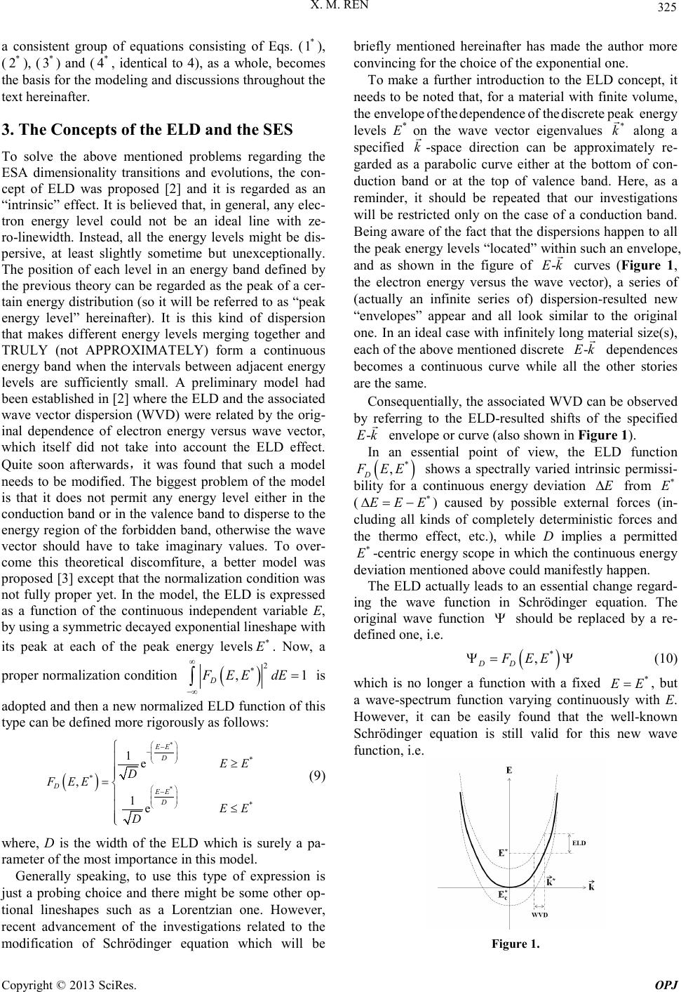

X. M. REN
325
a consistent group of equations consisting of Eqs. (
*
1
),
(
*
2
), (
*
3
) and (
*
4
, identical to 4), as a whole, becomes
the basis for the modeling and discussions throughout the
text hereinafter.
3. The Concepts of the ELD and the SES
To solve the above mentioned problems regarding the
ESA dimensionality transitions and evolutions, the con-
cept of ELD was proposed [2] and it is regarded as an
“intrinsic” effect. It is believed tha t, in general, any elec-
tron energy level could not be an ideal line with ze-
ro-linewidth. Instead, all the energy levels might be dis-
persive, at least slightly sometime but unexceptionally.
The position of each level in an energy band defined by
the previous theory can be regarded as the peak of a cer-
tain energy distr ibution (so it will be referred to as “peak
energy level” hereinafter). It is this kind of dispersion
that makes different energy levels merging together and
TRULY (not APPROXIMATELY) form a continuous
energy band when the intervals between adjacent energy
levels are sufficiently small. A preliminary model had
been established in [2] where the ELD and the associated
wave vector dispersion (WVD) were related by the orig-
inal dependence of electron energy versus wave vector,
which itself did not take into account the ELD effect.
Quite soon afterwards，it was found that such a model
needs to be modified. The biggest problem of the model
is that it does not permit any energy level either in the
cond uction b and o r in the val ence band to disperse to t he
energy region of the forbidden band, otherwise the wave
vector should have to take imaginary values. To over-
come this theoretical discomfiture, a better model was
proposed [3] except that the normalization condition was
not fully proper yet. In the model, the ELD is expressed
as a function of the continuous independent variable E,
by usin g a s ym metric decayed exponential lineshape with
its peak at each of the peak energy levels
*
E
. Now, a
proper normalization conditio n
( )
2
*
,1
D
FE EdE
∞
−∞
=
∫
is
adopted and then a new normali zed E LD funct ion o f this
type can be defined more rigorously as follows:
( )
*
*
*
*
*
1e
,
1e
EE
D
DEE
D
EE
D
F EE
EE
D

−
 −


−




≥


=

≤


(9)
where, D is the width of the ELD which is surely a pa-
rameter of the most importance in this model.
Generally speaking, to use this type of expression is
just a probing choice and there might be some other op-
tional lineshapes such as a Lorentzia n one. However,
recent advancement of the investigations related to the
modification of Schrödinger equation which will be
briefly mentioned hereinafter has made the author more
convi nc i ng fo r the choice of the exponential one.
To make a further introduction to the ELD concept, it
needs to be noted that, for a material with finite volume,
the envelope of the dependence of the discre te peak energy
levels E* on the wave vector eigenvalues * k

along a
specified
k

-space direction can be approximately re-
garded as a parabolic curve either at the bottom of con-
duction band or at the top of valence band. Here, as a
reminder, it should be repeated that our investigations
will be restricted only on the case of a conduction band.
Being aware of the fact that the dispersions happen to all
the pe ak e nerg y le vel s “located” within s uch a n e nvelo pe ,
and as shown in the figure of -Ek

curves (Figure 1,
the electron energy versus the wave vector), a series of
(actually an infinite series of) dispersion-resulted new
“envelopes” appear and all look similar to the original
one. In an ideal case with infinitely long material size(s),
each of the above mentioned discrete
-Ek

dependences
becomes a continuous curve while all the other stories
are the same.
Consequentially, the associated WVD can be observed
by referring to the ELD-resulted shifts of the specified
-Ek

envelope or curve (also shown in Figure 1).
In an essential point of view, the ELD function
( )
*
,
D
F EE
shows a spectrally varied intrinsic permissi-
bility for a continuous energy deviation
E∆
from
*
E
(
*
EEE∆= −
) caused by possible external force s (in-
cluding all kinds of completely deterministic forces and
the thermo effect, etc.), while D implies a permitted
*
E
-centric energy scope in which the continuous e nergy
deviation mentioned above could manifestly hap p e n.
The ELD actually leads to an essential change regard-
ing the wave function in Schrödinger equation. The
original wave function
Ψ
should be replaced by a re-
defined one, i.e.
( )
*
,
DD
F EEΨ= Ψ
(10)
which is no longer a function with a fixed
*
EE=
, but
a wave-spectrum function varying continuously with E.
However, it can be easily found that the well-known
Schrödinger equation is still valid for this new wave
function, i.e.
Figure 1.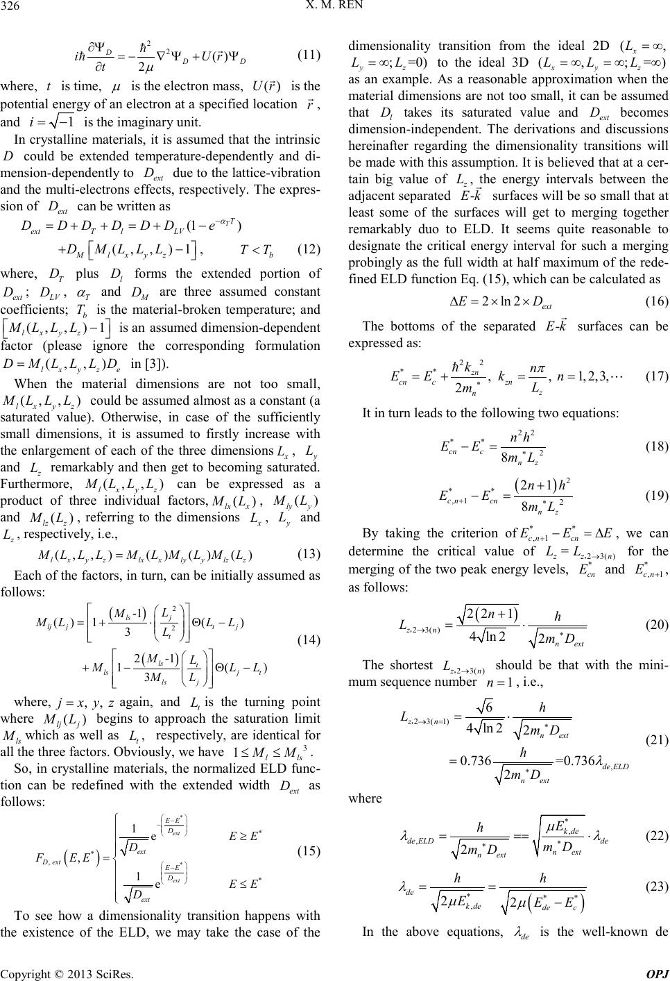

X. M. REN
326
22()
2
D
DD
i Ur
t µ
∂Ψ =−∇Ψ +Ψ
∂


(11)
where,
t
is time,
µ
is the electron mass,
()Ur

is the
potential energy of an electron at a specified location
r

,
and
1i=−
is the imaginary unit .
In crystalline materials, it is assumed that the intrinsic
D
could be extended temperature-dependently and di-
mension-dependently to ext
D
due to the la ttice -vibration
and the multi-electrons effects, respectively. The expres-
sion of ext
D
can be written as
(1 )
T
T
extT lLV
DDDD DDe
α −
=++=+−
(, , )1
M lxyz
D MLLL

+−

,
b
TT<
(12)
where, T
D
plus
l
D
forms the extended portion of
ext
D
;
LV
D
,
T
α
and
M
D
are three assumed constant
coefficients;
b
T
is the material-broken temperature; and
(, , )1
lxyz
MLLL

−

is an assumed dimension-dependent
factor (please ignore the corresponding formulation
(,,)
lxyz e
D MLLLD=
in [3]).
When the material dimensions are not too small,
(,,)
lxyz
MLLL
could be assumed almost as a constant (a
saturated value). Otherwise, in case of the sufficiently
small dimensions, it is assumed to firstly increase with
the enlargement of each of the three dimensions
x
L
,
y
L
and z L remarkably and then get to becoming saturated.
Furthermore,
(,,)
lxyz
MLLL
can be expressed as a
product of three individ ual facto r s,
()
lx x
ML
,
()
ly y
ML
and
()
lz z
ML, referring to the dimensions x L,
y
L
and
z
L, respectively, i.e.,
(,,)()()()
l xy zlx xlyylz z
MLLLM LM LM L=
(13)
Each of the factors, in turn, can be initially assumed as
follows:
( )
( )
2
2
-1
() 1()
3
2 -1
1()
3
j ls
lj jtj
t
ls t
lsj t
ls j
L
M
MLL L
L
ML
M LL
ML


=+⋅ Θ−
 






+ −Θ−
 




(14)
where,
, , j xyz=
again, and
t
L
is the turning point
where
()
lj j
ML
begins to approach the saturation limit
ls
Mwhi ch as well as t L, respectively, are identical for
all the three factors. Obviously, we have 3 1l ls
MM
≤≤ .
So, in crystalline materials, the normalized ELD func-
tion can be redefined with the extended width ext D as
follows:
( )
*
*
*
*
,
*
1e
,
1e
ext
ext
EE
D
ext
D extEE
D
ext
EE
D
F EE
EE
D

−

−


−




≥


=

≤


(15)
To see how a dimensionality transition happens with
the existence of the ELD, we may take the case of the
dimensionality transition from the ideal 2D
(,
x
L=∞
; =0)
yz
LL
= ∞ to the ideal 3D (,;=)
xyz
LLL=∞=∞ ∞
as an example. As a reasonable approximation when the
material dimensions are not too small, it can be assumed
that
l
D
takes its saturated value and ext
D becomes
dimension-independent. The derivations and discussions
hereinafter regarding the dimensionality transitio ns will
be made with thi s as sumptio n. It is believed that at a cer-
tain big value of z L, the energy intervals between the
adjacent separated
-Ek

surfaces will be so small that at
least some of the surfaces will get to merging together
remarkably duo to ELD. It seems quite reasonable to
designate the critical energy interval for such a merging
probingly as the full width at half maximum of the rede-
fined E LD fu nc ti on Eq. (15), which can be calculated as
2ln 2ext
ED
∆=× × (16)
The bottoms of the separated
-Ek

surfaces can be
expressed as:
22
**
, , 1,2,3,
2
zn
cn cznz
n
kn
EEkn
L m
π
∗
=+==

(17)
It in turn leads to the following two equation s:
22
**
2
8
cn c
nz
nh
EE mL
∗
−=
(18)
( )
2
**
,1 2
21
8
c ncn
nz
nh
EE mL
+∗
+
−=
(19)
By taking the criterion of
**
,1c ncn
EEE
+−=∆
, we can
determine the critical value of z L=
23()zn
L
→，
for the
mergi ng of t he two p eak ene rgy leve ls,
*
cn
E
and *
,1
cn
E+,
as follows:
( )
23( )
221
4ln 22
zn
n ext
nh
LmD
→∗
+
= ⋅
，
(20)
The shortest
23()zn
L
→，
should be that with the mini-
mum sequence number
1n=
, i.e.,
2 3(1)
,
6
4ln 22
0.736=0.736
2
zn
n ext
de ELD
n ext
h
LmD
h
mD
λ
→= ∗
∗
= ⋅
=
，
(21)
where
*,
,
2
k de
de ELDde
n ext
n ext
E
h
mD
mD
µ
λλ
∗
∗
=== ⋅
(22)
( )
***
,
22
de
k dede c
hh
EEE
λµµ == −
(23)
In the above equations, de λ is the well-known de

X. M. REN
327
Broglie wavelength with
*
de
E
and *,kde E being the av-
erage total energy and the average kinetic energy of an
electron, respectively, in a specified system, while
,de ELD
λ
is such a “golden quantity” that it times a fixed
proportional constant (
0.736
) simply equals the critical
size
2 3(1)zn
L
→=，
. We may name ,de ELD
λ
as “the nominal
de Broglie wavelength” referring to the dimensionality
transition due to its above mentioned feature as well as
its similar ity to de λ in mathematical expression.
We may also make
2 3(1)zn
L
→=，
explicitly related with
de
λ by writin g it as follows:
*,
2 3(1)
0.736
k de
z nde
n ext
E
LmD
µλ
→= ∗
= ⋅
，
(24)
In this equation, it has been shown so clearly how the
extended ELD width ext D serves as an objective tie
between de Broglie wavelength and the critical point of
the dimensionality transition and how de Broglie wave-
length plays its r ole in the quantum size effect.
Relevant experiments are needed to judge the truth-
fulness of the above mentioned theoretical assumptions
and predictions both qualitative ly and quantitatively.
In addition, owing to the above described effort of in-
quiring into the relationship between the concept of de
Broglie wavelength of electrons and the dimensionality
transition phenomena, the author has been further sus-
pecting the possibility if D would increase somehow with
the increasing of the peak energy level
*
E
. If this as-
sumption would be true, it might be found that we had
approached the bridge between the microcosm and the
macrocosm. Actually, if we deal with not only an elec-
tron but also a bigger particle or an object in a general
sense with arbitrary mass and energy, we may do a fur-
ther reasoning to assume the increasing of D with the
increases of both the mass and the energy of the
object, for example,
*
( )
n
D E µ ∝
with
n
being a pos-
itive rational number. Then, as a result, an object with a
big enough mass and a high enough energy would ma-
nifest a huge ELD and there no longer exists a
states-architecture of discrete energy levels. Instead, the
states-architecture of this kind of objects should be al-
ways continuous. It refers therefore to a non-quantum
world or a Ne wtonian world.
Even more additionally, as we comprehensively think
about the difference between the mechanical behaviors of
an object in the quantum regime and in the Newtonian
regime, it seems that another assumption in association
with the ELD should also be made: there might exist an
effect of SES, i.e. the spatial extension shrinkage as men-
tioned hereinabove. As we know, the Newtonian me-
chanics is deterministic while the quantum mechanics is
statistic. Therefore, the confinement tendency o f th e sp a-
tial extension of a n object should be enha nced d uring t he
evolut ion fro m the quant um mecha nics to the Newtonian
mechanics. Similarly to the above given descriptions of
( )
*
,
D
F EE
and
D
, the nomorlized SES function could
be assumed as
( )
2
*
3
42
3
2
*2
()
rr
S
S
Fr re
S
π
−
−
−=

 (25)
and the SES parameter
S
as the measure of the con-
fined exte nsio n could a lso be conceived as a function o f
*
E µ
and probingly could be
*
()n SE µ
−
∝
. Where,
*
r

is the spatia l position with the peak probability of ap-
pearance.
If this assumption of SES would be true, the wave
function should be changed further and, eventually,
Schrödinger equation should no longer be kept un-
changed; instead, it should have to be modified. At the
same time, Newtonian equation surely also needs to be
modified. Actually, the author has fulfilled both modifi-
cations a nd the relevant details will be described later.
Here given are the modified Schrödinger-Newtonian
equations themselves as follows:
( )( )
2
11
MM
DS
iDC EE
tE
∂Ψ ∂Ψ

−Θ− −Θ −

∂∂
 

(26-a)
( )
22
2
**
22
2
2()
2
12
1
M
M
DS DS
DS
Ur
rr rr
i CpC
SS C
µ

− ∇Ψ


= +Ψ



−−

+ ⋅−



+







 


( )( )
( )
1
22
2
(/)
/, 1
MM
EM
v
VFr Vvv
t
vv
v CV
tE
γ
µ
ξ
µξ
−
Ψ
Ω→∞ Ω→∞
Ψ
Ω→∞

Ψ ⋅Ψ=⋅




∂
+ =+Ψ 

∂



∫∫∫ ∫∫∫
∫∫∫


d
dd
d
d
d
d
(26-b)
where,
M
Ψ
is the modified wave function;
*
E EE=

the normalized energy;
p


the unit vector along the do-
minant momentum direction;
( )
Fr

the field of force;
v

the velocity vector;
( )
xΘ

a modified Heaviside
function of
x
with
( ) 0 12
+
Θ =

; DS C and
E
C
are
two constants; and,
1, 0, 1 γ = −
(case-dependent).
As a fully natural consequence of the formulation of
the modified Schrödinger equation, i.e. Eq.(26-a), one
essential relation,
*1 *
= =
S DS
S C ECE µµ
−

, has
been obtained a nd the other one,
*
D
DC E µ =
, has also
been assumed tentatively (both
S
C
and
D
C
are con-
stants). Th e two relations make the concepts of ELD/SES
quantitatively defined and lead to an important idea that
*
E µ
could be taken as the measure of the cosmo-level
(the author suggests to call it the “cosmicality”).
The above given modified Schrödinger-Newt onian
equations should be well valid in the mid-cosmic regime

X. M. REN
328
(between the microcosm and the macrocosm) where no
relativistic effect would need to be taken into account.
However, in the super-high speed regime, Einstein’s
theory of rela tivity featur ing an upper limit of veloc ity
c
should be adopted to make further modification of this
pair of equatio ns. I n associatio n with this conside ratio n, a
more unusual idea came out and had greatly surprised the
author: there mu st app ear a similar t heory of relativity for
super-low speed regime featuring a lower limit of veloc-
ity (LLV)
ˆ
c
! T his idea is nece ssar y not onl y for the fur-
ther modificatio n of the equations in the s uper-lo w speed
regime and the unveiling of a philosophical beauty of the
cosmic symmetry but also for the essential causal inter-
pretation of the statistical spatial extension of a particle,
or the so-called “probability wave” phenomenon. It
might be this lower-limit effect that intrinsically makes
any particle keeping un-static or in continuous motion
directed randomly. T he autho r su ggests to call t he matter
moving with the velocity
ˆ
c
, if it would exist, as “sy-
might” (it is similar to “light” but the first three letters
are newly introduced to replace “l” and to signalize that
it is a symmetrical existence for “light”; and, the word
rega rding i ts par ticle-property corresponding to “photon”
could be “symiton”) and to call
ˆ
c
itself the velocity of
symight. Consequentially, Einstein’s theory of relativity
can be reasonably modified with an extended Lorentz
transformation as follows:
( )
2
2
ˆ
1
1
c
v
xx vtv
c

−

′= −
−

(27-a)
22
2
222
ˆ
ˆ
1
ˆ
111
xv c
cvc v
v
tt vvc
ccv

 
 −

 
−  

 
′= −
  
−− ⋅−
  
  
(27-b)
And then, the mass
µ
should be expressed as:
2
mi 2
ˆ
1
1
d
c
v
v
c
µµ

−

=
−

(28)
In these relativistic equations,
v
is the velocity and
mid
µ
is the mass at the critical mid-cosmic velocity
ˆ
mid
v cc=
and is used to replace the static mass
0
µ
(or
0
m
) in Einstein’s theo ry of relativity.
As we can imagine, it should be difficult to directly
determine the lower limit velocity
ˆ
c
. Ho we ver , an indi-
rect method for the determination of
ˆ
c
with assistance
of the critical mid-cosmic velocity mid v could be
somewhat easy. Actually,
ˆ
c
can be determined from
( )
2
1
ˆ
mid
cc v
−
=
when mid
v
is known. In turn, mid
v
can
be determined by measuring
S
or
D
as precisely as
possible in a certain range of
v
around mid v.
Combining this essentially extended theory of relativ-
ity, or more explicitly the fu ll velocity-scope theory of
relativity, with the modified Schrödinger-Newton ian
equations given as Eq.(26) is so per fective and enligh-
tening that it makes the latter (a) being more rigorously
valid for all the possible cases especially in the su-
per-high and super-low speed regimes regarding the par-
ticles or objects in a common sense, and (b) probably
even being valid in t he velo cit y re gimes upwards beyond
c
and downwards beyond
ˆ
c
where, as the author sus-
pected, a new matter featuring an imaginary mass might
exist in a certain variety of intriguing forms. The p rope r-
ties a nd be havior s of t he new matter could be i nterpreted
with the aid of properly modified ELD and SES func-
tions and we may find that the imaginary mass could
actually make sense. This “new-matter” prediction could
hopefully conclude or at least share the century-long
challenges to Einstein’s prediction regarding the up-
per-limit velocity. I t is believed that any common par tic le
or object cannot surpass or just reach the velocity limits
c
and ˆ c indeed, while for the new matter, it is no
problem at all to manifest a velocit y beyond
c
or
ˆ
c
, or
furthermore, there are actually no other choices for the
new matter except moving essentially wit h a velocity
either higher than
c
or lower than
ˆ
c
. The key point
here is that different matters b ehave differ ently .
4. The DOS Expressions in the Dispersive
Cases
To make it convenient, we may refer the two cases, be-
fore and after the intro duction of ELD model, as “the d is-
persion-free case” and “the dispersive case”, respectively.
And, the values of the electron energy in the two cases
need to be denoted with different symbols, E* and E, als o
respectively. Then, in the dispersive case, Eqs. (
*
1
), (
*
2
),
(
*
3
) and (
*
4
, identical to 4) should be replaced respec-
tively by the following new expressions (just taking
( )
2*
,
,
D ext
F EE
as the typical convolute int egration factor):
( ) ()( )
( )
( )
*
*
*
*
*
*
2* **
,,
3
2 2** **
23
2* **
2
** **
,
8 2()
{[ e
e]
e}
c
ext
c
ext
ext
c
c DDextc
E
EE
ED
ncc
ext E
EE
D
c
E
EE
D
cc
E
EFE EEdE
mEEEE dE
D
EEdE
EE EEdE
ρρ
π
∞

−
∗−



−
∞



−
∞


=
= Θ−−
+−
+Θ −−
∫
∫
∫

∫
(29)

X. M. REN
329
( )
() ()
( )
( )
*
*
*
2 ***
,,
-2
*
2
2*
,, ,
4e
{[1-]
2
1
e}
2
c
cn
ext
cn
ext
c DzDextcz
E
EE
D
ncn
n
z
EE
D
cn
ELFEEE LdE
mEE
L
EE
ρρ
π
∞

−


∗

−



=
= Θ−
+ Θ−
∫
∑
 (30)
( )
() ()
( )
( )
*
*
*,
*
,
2 ***
,
2*,*
**
,,
2*,*
**
,
,,
, ,,
e
2
{
e
c
ext
c mn
ext
cDy z
D extcyz
E
EE
D
Ec mn
n
mn
ext y zEc mn
EE
D
c mn
Ec mn
EL L
FE EELLdE
EE
mdE
D LLEE
EE dE
EE
ρ
ρ
π
∞

−
 −
 ∗

−



∞
=


Θ−

=
−





Θ−

+
−



∫
∑∫
∫

( )
*
*,
2*,*
**
,
e }
ext
c mn
EE
D
c mn
Ec mn
EE
dE
EE

−



∞


Θ−

+
−



∫
(31)
( )
() ()
( )
( )
*
*,
*,
,
2 ***
,
2*,
,,
2*,
,,,
, ,,,
2
[e
e]
c
c lmn
ext
c lmn
ext
cDx y z
D extcxyz
E
EE
D
c lmn
lmn
ext x y z
EE
D
c lmn
EL LL
FEEELLLdE
EE
D LLL
EE
ρ
ρ
∞

−

−


−



=
= Θ−
+ Θ−
∫
∑
(32)
Among all these four expressions, Eq.(32) is uniquely
a general one which is applicable to all the cases includ-
ing the bul k, q uantu m wel l, wire a nd do t materials; while,
the others, in a rigorous sense, are applicable only to
those specified ideal cases where there should be three
dimensions, two dimensions or at least one dimension
reaching infinity (please ignore Eqs.(6) and (7) in [3]).
5. The Accurate and Comprehensive
Understanding of the Dimensionality
Evolution
1) In the ideal 3D case corresponding to Eq.(29), the size
of the material along each direction reaches its upward
limit, so the individual contribution from each of the
three sizes to the identification number of the dimensio-
nality (dimensionality ID-number) should be unity and
thus the dimensionality ID-number itself as the sum of
those contributions is “3”. As an alternative denotation,
we may also define a triplet of dimensionality indices
(DI-triplet) as [1,1,1] to separately specify the 3 fold
contribution s.
2) As to Eq.(30), it is the case that the dimensionality
ID-number varies from 2 (the ideal 2D, 0
z
L=) to 3 (the
ideal 3D, z L=∞). A rigorous critical point
23
z
L→，,
whic h should be ne ar but not exactly identica l to the val-
ue of
2 3(1)zn
L
→=，
given in Section 3, can be determined
by a method of similarity calculation [2-3]. The defini-
tion of t he Si mi lari ty Function for
( )
,
,
cDz
EL ρ
is given as:
()()
()( )
( )
,
,2
,
[,, ]
cDzr
cDzr
r
E LEdE
SEL E
E dE
ρ
ρρ
ρρ
ρ
∞
−∞
∞
−∞
=∫
∫
(33)
where,
( )
r
E ρ
is a proper reference function case by
case.
Then, the criterion for the rigorous determination of
23
z
L→， should be as
( )()
()( )
,
,
[ ,,,]
[,, ]
cD zcz
cD zc
S ELEL
S ELE
ρ
ρ
ρρ
ρρ
≠∞ ≠∞
= ≠∞
(34)
A fractional dimensionality ID-number corresponding
to the critical point
23z
L
→，
should be naturally the mid-
point between the numbers of 2 and 3, i.e. should be
equa l to 2 .5 . Then, the di mensio nality ID -numbers within
the 2D and 3D regions should be (2 - 2.5) and (2.5 - 3),
respectively. We can also use the relevant DI-triplets,
written as [1,1, z
d], to denote the dimensio nalities men-
tioned above, where z d has been defined in [3] as fol-
lows:
( ) ( )
( )
,, 23
2, 23
( 0.5)
2
cDzcDz
z
cD z
ELEL dE
d
E LdE
ρρ
ρ
∞
→
−∞
∞
→
−∞
≤=
∫
∫
，
，
，，
，
(35)
()( )
( )
,, ,0
2, ,0
- I
( 0.5)0.5
2 - I
cDz cDz
z
cDz
ELE dE
d
E dE
ρρ
ρ
∞
−∞
∞
−∞
≥=+ 


∫
∫
，
(36)
where,
( )
( )
,0,23,
I
zcDz cD
ELE dE ρρ
∞
→
−∞
=
∫，
，
(37)
The dimensionality ID-numbers can be derived from
the corresponding DI-triplets by si mply taking the s um of
the indices, i.e .
2
z
d+
.

X. M. REN
330
3) As to Eq.(31), it refers to a complicated case. When
0
z
L=
and
y
L
varies, similarly to the discussion re-
garding Eq.(30), the dimensionality ID-number can va-
ries from 1 ( the ideal 1D, Ly = 0) to 2 (the ideal 2D, Ly =
∞). The fractional dimensionality ID-number corres-
ponding to the critical point
,1 22 3
()
yz
LL
→→
=
，
for the
transition fro m 1D to 2D regions sho ul d be 1.5. T hen, the
dimensionality ID-numbers within the 1D and 2D re-
gions should be (1 - 1.5) and (1.5 - 2), respectively. The
corresponding DI-triplet should be [1, y
d, 0]. If 0
z
L≠,
the situation is quite different. It is impossible to consis-
tently define a single dimensionality ID-number for an
arbitrary combination of z
L and
y
L
. So, the DI-trip-
lets, i.e. [1,
y
d
, z
d] becomes the unique choice for the
dimensionality denotation. All the possible dimensional-
ity regions can be defined as D1: [1, 0.5
y
d<,
0.5
z
d<]; D2: [1,
0.5
y
d>
, 0.5
z
d<] or [1, 0.5
y
d<,
0.5
z
d>]; and D3: [1,
0.5
y
d>
, 0.5
z
d>].
4) Quite similarly but referring to a more complicated
case, Eq.(32) can be interpreted as follows: When
0
zy
LL= =
and only
x
L
varies, the dimensionality
ID-numbers can varies fro m 0 (the ide al 0D, Lx = 0) to 1
(the ideal 1D, Lx = ∞). The fractional dimensionality
ID-number corresponding to the critical point 01
(
x
L→=
，
12 23
)
yz
LL
→→
=
，，
for the transition fro m 0D to 1D regions
should be 0.5. Then, the dimensionality ID-numbers
withi n the 0D and 1D regions should be (0 - 0.5) and ( 0.5
- 1), respectively. The corresponding DI-triplets should
be [
x
d
,0, 0]. If
0
z
L≠
and
0
y
L≠
, the dimensionality
should be denoted only by the DI-triplets, i.e. [
x
d
,
y
d
,z
d]
and the dimensionality regions can be defined as D0:
[0.5
x
d<,0.5
y
d<,0.5
z
d<]; D1:[0.5
x
d>,0.5
y
d<,
0.5
z
d<], [0.5
x
d<,
0.5
y
d>
, 0.5
z
d<] or
[0.5
x
d<,0.5
y
d<,0.5
z
d>]; D2:[ 0.5
x
d>,
0.5
y
d>
,
0.5
z
d<], [0.5
x
d<,
0.5
y
d>
, 0.5
z
d>] or
[0.5
x
d>, 0.5
y
d< ,0.5
z
d>]; and D3
[0.5
x
d>, 0.5
y
d>
,0.5
z
d>].
6. Discussions and Conclusions
This work has provided a novel understanding of ESA
and its di mensionality in semiconductors or cryst alline
materials; has established a more reasonable and con-
vincing basis for further development of nanohetero-
structure physics, especially the hetero-dimensional
structure physics; has made three new assumptions of the
ELD, the SES and the LLV; has led to a new quantum-
and furthermore a full cosmic-scope mechanical picture,
a pair of the modified Schrödinger-Newtonia n equatio n s
being valid thr ou gho ut the ev olution from the microcos m
regime to the macrocosm regime, an idea and the initial
efforts to establish a theory of super-lo w-speed rela tivit y,
and a “new-matter” pr e d ic tion. Some fundamental phe-
nomena such as the tunneling effect can be modeled
more accurately and becomes more understandable by
adopting the ELD assumption. Expected should also be
the possible inventions of some novel electronic and op-
toelectronic devices. For example, it seems quite reason-
able to predict a DOS gradient caused electron (or more
generally, carrier) diffusion in a hetero-dimensional
structure or a structure featuring a gradually changed
dimensionality. Then a sort o f nove l se miconduc tor e lec-
tronic devices featuring the mono-carrier transportation
(recombination free) and the remarkably reduced power
consumption can be conceived and demonstrated, while
relevant works have been on its way in the author’s la-
boratory.
7. Acknowledgements
I would like to express my deep gratitude to Prof. Zh. I.
Alfer ov for hi s enlig htening words. I am also very grate-
ful to Prof. V. G. Dubr ovs kii for his conc ent rate d d iscus-
sion on this topic as well as his warm encouragement, to
Researcher YE Xiaoyan for her all the way support and
helpful suggestions, to my colleagues in my group as
well as other s in the uni versit y, inc lud ing Associate Prof.
WANG Qi, Associate Prof. DUAN Xiaofeng, Prof.
HUANG Yongqing, Prof. ZHANG Xia, Associate Prof.
WANG Jun, Mr. CAI Shiwei, Mr. HAO Jiaquan, Mr.
WANG Jin, Prof. FANG Binxing, and Prof. WANG Ya-
jie for their valued supports and re le va nt discussion s, and
to Ms. LUO Fen as well as some of my students, espe-
cially Mr. LIU Xiao long, Mr. JIA Zhigang and Mr. YAN
Xin, for their precious helps and necessary assistances.
This work has been supported by the National Basic Re-
search Program of China (No. 2010CB327601), the Na-
tional Natural Science Foundation of China (No.
61020106007, 61108048), International Science &
Technology Cooperation Program of China (No.
2011DFR11010) and the 111 Project (No. B07005).
REFERENCES
[1] Zh. I. Alferov, “The Double Heterostructure: Concep t and
Its Applications in Physics, Electron ics and Technology”,
Nobel Lectu r e, December 8, 2000.
[2] X. M. Ren, “Theoretical Investigation on the Continuous
Evolution of the Electron-Gas Dimensionality: From
Bulk Materials to Quantum Dots” (postdeadline paper),
2012 Asia Communication and Photonics Conference,
November 7-11, 2012.
[3] X. M. Ren, “Modification of the Theory on the Ener-
gy-Level Dispersion and the Continuity of the Elec-
tron-Gas Dimensionality” (invited talk / plenary session;
to be delivered), 21st International Symposium on Nano-
structures: Physics and Technology, June 24-28, 2013.