The Economic Motion

doi:10.4236/tel.2013.34042

Paper Menu >>

Journal Menu >>

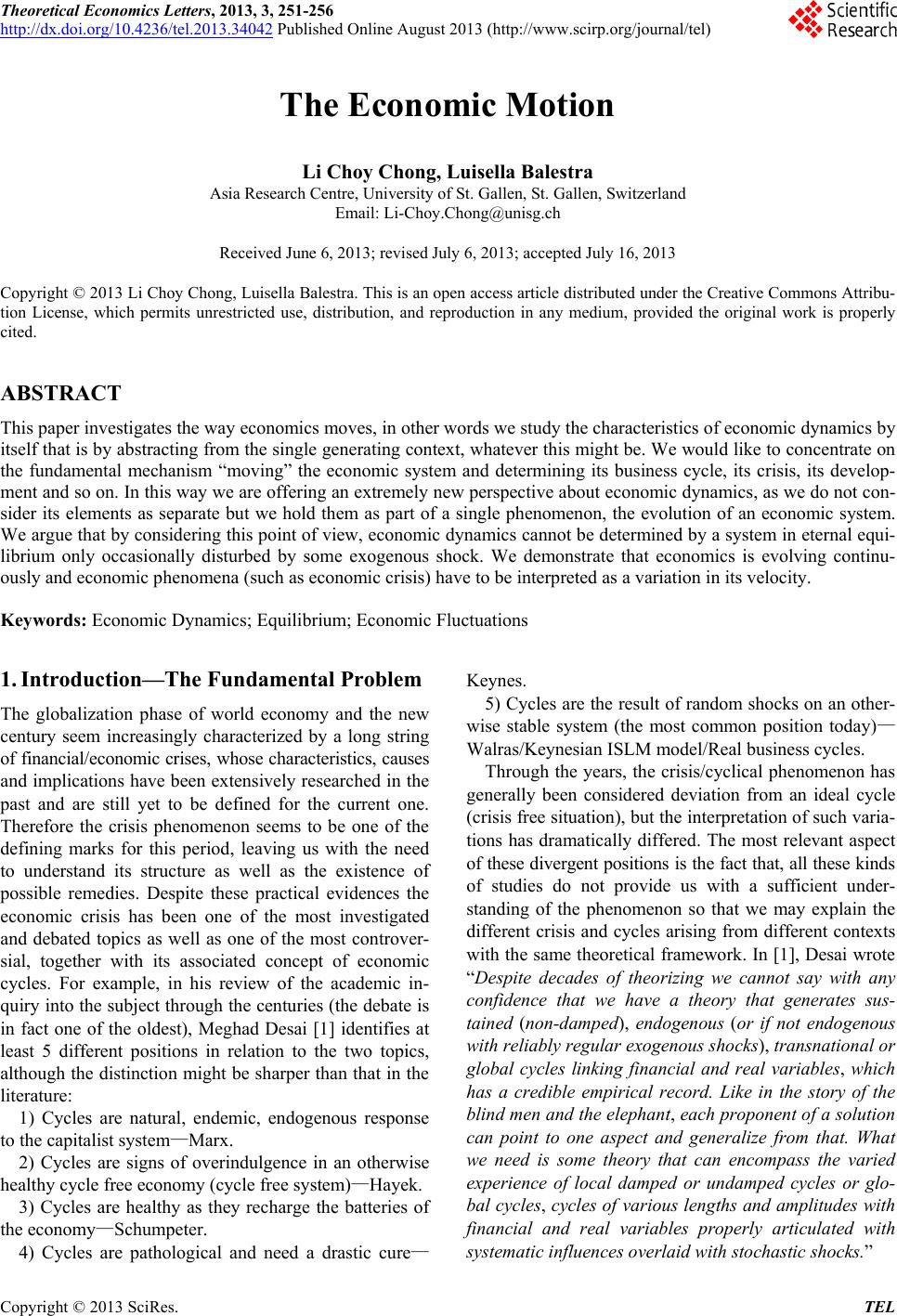Theoretical Economics Letters, 2013, 3, 251-256

http://dx.doi.org/10.4236/tel.2013.34042 Published Online August 2013 (http://www.scirp.org/journal/tel)

The Economic Motion

Li Choy Chong, Luisella Balestra

Asia Research Centre, University of St. Gallen, St. Gallen, Switzerland

Email: Li-Choy.Chong@unisg.ch

Received June 6, 2013; revised July 6, 2013; accepted July 16, 2013

tion License, which permits unrestricted use, distribution, and reproduction in any medium, provided the original work is properly

cited.

ABSTRACT

This paper investigates the way economics moves, in other words we study the characteristics of economic dynamics by

itself that is by abstracting from the single generating context, whatever this might be. We would like to concentrate on

the fundamental mechanism “moving” the economic system and determining its business cycle, its crisis, its develop-

ment and so on. In this way we are offering an extremely new perspective about economic dynamics, as we do not con-

sider its elements as separate but we hold them as part of a single phenomenon, the evolution of an economic system.

We argue that by considering this point of view, economic dynamics cannot be determined by a system in eternal equi-

librium only occasionally disturbed by some exogenous shock. We demonstrate that economics is evolving continu-

ously and economic phenomena (such as economic crisis) have to be interpreted as a variation in its velocity.

Keywords: Economic Dynamics; Equilibrium; Economic Fluctuations

1. Introduction—The Fundamental Problem

The globalization phase of world economy and the new

century seem increasingly characterized by a long string

of financial/economic crises, whose characteristics, causes

and implications have been extensively researched in the

past and are still yet to be defined for the current one.

Therefore the crisis phenomenon seems to be one of the

defining marks for this period, leaving us with the need

to understand its structure as well as the existence of

possible remedies. Despite these practical evidences the

economic crisis has been one of the most investigated

and debated topics as well as one of the most controver-

sial, together with its associated concept of economic

cycles. For example, in his review of the academic in-

quiry into the subject through the centuries (the debate is

in fact one of the oldest), Meghad Desai [1] identifies at

least 5 different positions in relation to the two topics,

although the distinction might be sharper than that in the

literature:

1) Cycles are natural, endemic, endogenous response

to the capitalist system—Marx.

2) Cycles are signs of overindulgence in an otherwise

healthy cycle free economy (cycle free system)—Hayek.

3) Cycles are healthy as they recharge the batteries of

the economy—Schumpeter.

4) Cycles are pathological and need a drastic cure—

Keynes.

5) Cycles are the result of random shocks on an other-

wise stable system (the most common position today)—

Walras/Keynesian ISLM model/Real business cycles.

Through the years, the crisis/cyclical phenomenon has

generally been considered deviation from an ideal cycle

(crisis free situation), but the interpretation of such varia-

tions has dramatically differed. The most relevant aspect

of these divergent positions is the fact that, all these kinds

of studies do not provide us with a sufficient under-

standing of the phenomenon so that we may explain the

different crisis and cycles arising from different contexts

with the same theoretical framework. In [1], Desai wrote

“Despite decades of theorizing we cannot say with any

confidence that we have a theory that generates sus-

tained (non-damp ed), endogenous (or if not endogenous

with reliably regular exogenous shocks), transnational or

global cycles linking financial and real variables, which

has a credible empirical record. Like in the story of the

blind men and the elephan t, each proponen t of a solution

can point to one aspect and generalize from that. What

we need is some theory that can encompass the varied

experience of local damped or undamped cycles or glo-

bal cycles, cycles of various lengths and amplitudes with

financial and real variables properly articulated with

systematic influences overlaid with stochastic shocks.”

L. C. CHONG, L. BALESTRA

252

In other words, current theories are unable to offer a

scientific explanation about the fact that “economics

changes” (and sometimes sodramatically as in these

years), since all of them are too restricted by the limits

determined by the particular situations they are trying to

explain and therefore for them it’s impossible to give

insights that we can better adopt in different contexts

than the generating one. We think that the main problem

is the fact that a more comprehensive perspective in eco-

nomic theory is missing: all the economic dynamics phe-

nomena, such as crisis, are considered as separated events

and therefore we cannot get a “truly” scientific explana-

tion for them as we are limited by each generating context.

Aim of this paper is to overcome this problem; we

want to explain the way economics moves by consider-

ing each economic dynamics elements as particular ex-

pressions of a more general phenomenon, that is the

evolution of an economic system. In this way, we show

first the impossibility of an equilibrium position and

therefore of an ideal crisis free situation (=the eternal

steady state), second we develop a new scientific para-

digm based upon the speed concept, then, through the

empirical observations about the US economy from 1960

to 2010, we subsequently show and prove that economic

crisis as well as growth episodes can in effect be inter-

preted as variations in the velocity of the system. Thus,

no matter the originating cause of the particular situation

(we analyse 50 years), a general explanation for eco-

nomic dynamics is empirically tested and confirmed,

being therefore able to move over from the limits implied

by the usual exogenous shock scheme. It’s a very inno-

vative work due to our approach: we treat economic dy-

namics as a motion phenomenon by itself, therefore try-

ing to abstract from any generating context and deriving

from this some general (=scientific) insight about the

evolution of an economic system.

2. Economic Dynamics as the Motion of an

Economic System

The fundamental element characterizing our approach to

the problem is the fact that economic crisis, equilibrium,

shocks, growth, cycles and the like, are all movements of

a system [2,3]. In fact, we can always observe asystem,

which could be defined as a configuration of variables

within a specific space and at a specific point in time and

such a correlated structure of variables specified and

changing with the time element would provide a frame of

reference to compare with, as it moves from one con-

figuration to another and thereby expressing the fact that

it is changing its position. A consequent aspect of interest

would have us understand that if it’s moving, the system

must be expressed per definition by the elements of time,

space (s, the length of path travelled until time t) and

speed1, the time derivative of s that is:

 (1)

Despite these general evidences, the traditional ap-

proach about economic dynamics is quite paradoxically

characterized by the lack of awareness about the fact that

economic phenomena are in effect motions in a specific

space. In fact the fundamental tool used for expressing

economic motion has so far been the equilibrium that is

the motionlessness of the economic system. Equilibrium

represents a very common scientific paradigm for eco-

nomictheory, since this state of nature is usually treated

as the best solution to be achieved by economics and it

offers the basis for three kinds of “movements”:

 Base—unit movement of the system defined by the

achievement of a position of equilibrium(e.g. the sin-

gle market or general market equilibrium, as the tran-

sition to a different position in the temporal evolution

for economics)2;

 motion obtained through the temporal repetition of an

equilibrium position. It is determined by the repetition

of a base unit movement (usually a goal equilibrium)

over a (infinite) time horizon after having specified a

law of transition for the system. We usually end up

with a condition describing a path made by a fixed

sequence of equilibrium position, which is supposed

to remain unchanged for the time being (such as Euler

condition);

 exogenous shocks. Together with the expected value

operator, represents the uncertainty inside economics,

making it impossible to predict outcomes. The ex-

ogenous shock gives the impulse for the economic

surrounding context to vary and its main effect is a

displacement of the system’s path in the economic

space or in its structure. In any case it has to be con-

sidered as a temporally limited event that becomes

eventually absorbed by the system through the defini-

tion of new characteristics of the model (or for the

path), that is supposed to remain again “eternally” un-

altered thereafter, unless some other exogenous shock

will come around another time.

According to the definition of Fritz Machlup [4] equi-

librium is a “constellation of selected interrelated vari-

ables so adjusted to one another that no inherent ten-

dency to change prevail in the model which they consti-

tute”. As Chiang [5] pointed out, this explanation implies

a relation among selected variables such that they are in a

1We can also consider acceleration 0

limt



a

.

2The maximization assumption also expresses this kind of motion (it’s a

goal equilibrium) and in this perspective the comparative static analysis

and the existence of rigidities in the relationship

etween variables have

to be interpreted as the definition of different paths and outputs toward

(or not toward) this state for the economic system.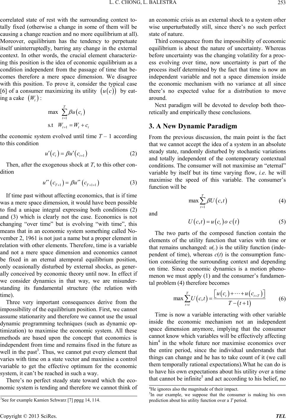

L. C. CHONG, L. BALESTRA 253

correlated state of rest with the surrounding context to-

tally fixed (otherwise a change in some of them will be

causing a change reaction and no more equilibrium at all).

Moreover, equilibrium has the tendency to perpetuate

itself uninterruptedly, barring any change in the external

context. In other words, the crucial element characteriz-

ing this position is the idea of economic equilibrium as a

condition independent from the passage of time that be-

comes therefore a mere space dimension. We disagree

with this position. To prove it, consider the typical case

[6] of a consumer maximizing its utility by eat-

ing a cake













s.t

max









the economic system evolved until time T ‒ 1 according

to this condition







uc uc







t



11T

(2)

Then, after the exogenous shock at T, to this other con-

dition

 

uc uc









 (3)

If time past without affecting economics, that is if time

was a mere space dimension, it would have been possible

to find a unique integral expressing both conditions (2)

and (3) which is clearly not the case. Economics is not

changing “over time” but is evolving “with time”, this

means that in an economic system something called No-

vember 2, 1961 is not just a name but a proper element in

relation with other elements. Therefore, time is a variable

and not a mere space dimension and economics cannot

be fixed in an eternal atemporal equilibrium position,

only ocasionally disturbed by external shocks, as gener-

ally conceived by economic theory until now. In effect if

we consider dynamics in that way, we are misunder-

standing its fundamental structure (the relation with

time).

Three very important consequences derive from the

impossibility of the equilibrium position. First, we cannot

assume stationarity and therefore we cannot use the usual

dynamic programming techniques (such as dynamic op-

timization) to maximise the economic system. All these

methods are based upon the concept that economics is

independent from time and remains fixed in the future as

well in the past3. Thus, we cannot put every element that

varies with time on a state vector and maximise a control

variable to get the effective optimum for the economic

system, it can’t be reached in such a way.

There’s no perfect steady state toward which the eco-

nomic system is tending and therefore we cannot think of

an economic crisis as an external shock to a system other

wise unperturbatedly still, since there’s no such perfect

state of nature.

Third consequence from the impossibility of economic

equilibrium is about the nature of uncertainty. Whereas

before uncertainty was the changing volatility for a proc-

ess evolving over time, now uncertainty is part of the

process itself determined by the fact that time is now an

independent variable and not a space dimension inside

the economic mechanism with no variance at all since

there’s no expected value for a distribution to move

around.

Next paradigm will be devoted to develop both theo-

retically and empirically these conclusions.

3. A New Dynamic Paradigm

From the previous discussion, the main point is the fact

that we cannot accept the idea of a system in an absolute

steady state, randomly disturbed by stochastic variations

and totally independent of the contemporary contextual

conditions. The consumer will not maximise an “eternal”

variable by itself but its time varying flow, i.e. he will

maximise the speed of this variable. The consumer’s

function will be



max ,

Uct





 (4)

and











Uctuc oct

(5)

The two parts of the composed function contain the

elements of the utility function that varies with time or

that remains unchanged: u(.) is the utility function (inde-

pendent of time), whereas c(t) is the consumption func-

tion considering the surrounding context and depending

on time. Since economic dynamics is a motion pheno-

menon we must apply (1) and the consumer’s fundamen-

tal problem (4) therefore becomes



 



max ,1

Ttt

uc uc

Uct Tt



















(6)

Time is now a variable interacting with other variable

inside the economic mechanism not an independent

space dimension anymore, implying that the consumer

cannot know which variables will be effectively affecting

him4 in the whole future nor maximise economics over

the entire period, since the individual understands that

things can change and he has to take count of it (we call

them temporally rational expectations).What he can do is

to have his own expectations about his utility over a time

that cannot be infinite5 and act according to his belief, no

4He ignores also the magnitude of their impact.

5In our example, we suppose that the consumer is making his own

rediction about his utility function over a T period.

3See for example Kamien Schwarz [7] ppgg 14, 114.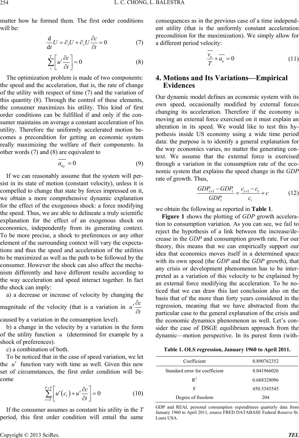

L. C. CHONG, L. BALESTRA

254

matter how he formed them. The first order conditions

will be:

dtc

UUU



 

 (7)















 (8)

The optimization problem is made of two components:

the speed and the acceleration, that is, the rate of change

of the utility with respect of time (7) and the variation of

this quantity (8). Through the control of these elements,

the consumer maximizes his utility. This kind of first

order conditions can be fulfilled if and only if the con-

sumer maintains on average a constant acceleration of his

utility. Therefore the uniformly accelerated motion be-

comes a precondition for getting an economic system

really maximizing the welfare of their components. In

other words (7) and (8) are equivalent to

a (9)

If we can reasonably assume that the system will per-

sist in its state of motion (constant velocity), unless it is

compelled to change that state by forces impressed on it,

we obtain a more comprehensive dynamic explanation

for the effect of the exogenous shock: a force modifying

the speed. Thus, we are able to delineate a truly scientific

explanation for the effect of an exogenous shock on

economics, independently from its generating context.

To be more precise, a shock to preferences or any other

element of the surrounding context will vary the expecta-

tions and thus the speed and acceleration of the utilities

to be maximized as well as the path to be followed by the

consumer. However the shock can also affect the mecha-

nism differently and have different results according to

the way acceleration and speed interact together. In fact

the shock can imply:

a) a decrease or increase of velocity by changing the

magnitude of the velocity (that is a variation in c







caused by a variation in the consumption level).

b) a change in the velocity by a variation in the form

of the utility function (determined for example by a

shock of preferences).

c) a combination of both.

To be noticed that in the case of speed variation, we let

the function vary with time as well. Given this new

set of circumstances, the first order condition will be-

come

u



ucu t























(10)

If the consumer assumes as constant his utility in the T

period, this first order condition will entail the same

consequences as in the previous case of a time independ-

ent utility (that is the uniformly constant acceleration

precondition for the maximization). We simply allow for

a different period velocity:



 (11)

4. Motions and Its Variations—Empirical

Evidences

Our dynamic model defines an economic system with its

own speed, occasionally modified by external forces

changing its acceleration. Therefore if the economy is

moving an external force exercised on it must explain an

alteration in its speed. We would like to test this hy-

pothesis inside US economy using a wide time period

data: the purpose is to identify a general explanation for

the way economics varies, no matter the generating con-

text. We assume that the external force is exercised

through a variation in the consumption rate of the eco-

nomic system that explains the speed change in the GDP

rate of growth. Thus,

11tttt

GDPGDPcc c

GDP c







(12)

we obtain the following as reported in Table 1.

Figure 1 shows the plotting of GDP growth accelera-

tion to consumption variation. As you can see, we fail to

reject the hypothesis of a link between the increase/de-

crease in the GDP and consumption growth rate. For our

theory, this means that we can empirically support our

idea that economics moves itself in a determined space

with its own speed (the GDP and the GDP growth), that

any crisis or development phenomenon has to be inter-

preted as a variation of this velocity to be explained by

an external force modifying the acceleration. To be no-

ticed that we can draw this last conclusion also on the

basis that of the more than forty years considered in the

regression, meaning that we have abstracted from the

particular case to the general explanation of the crisis and

the economic dynamics phenomenon as well. Let’s con-

sider the case of DSGE equilibrium approach from the

dynamic—motion perspective. In its purest form (with-

Table 1. OLS regression, January 1960 to April 2011.

Coefficient 0.890762352

Standard error for coefficient 0.041966026

R2 0.688328096

F 450.5345545

Degree of freedom 204

GDP and REAL personal consumption expenditures quarterly data from

January 1960 to April 2011, source FRED DATABASE Federal Reserve St.

Louis USA.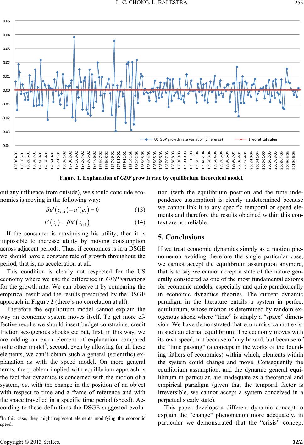

L. C. CHONG, L. BALESTRA

255

‐0.04

‐0.03

‐0.02

‐0.01

0.00

0.01

0.02

0.03

0.04

0.05

1960‐04‐01

1961‐05‐01

1962‐06‐01

1963‐07‐01

1964‐08‐01

1965‐09‐01

1966‐10‐01

1967‐11‐01

1969‐01‐02

1970‐02‐02

1971‐03‐02

1972‐04‐02

1973‐05‐02

1974‐06‐02

1975‐07‐02

1976‐08‐02

1977‐09‐02

1978‐10‐02

1979‐11‐02

1981‐01‐03

1982‐02‐03

1983‐03‐03

1984‐04‐03

1985‐05‐03

1986‐06‐03

1987‐07‐03

1988‐08‐03

1989‐09‐03

1990‐10‐03

1991‐11‐03

1993‐01‐04

1994‐02‐04

1995‐03‐04

1996‐04‐04

1997‐05‐04

1998‐06‐04

1999‐07‐04

2000‐08‐04

2001‐09‐04

2002‐10‐04

2003‐11‐04

2005‐01‐05

2006‐02‐05

2007‐03‐05

2008‐04‐05

2009‐05‐05

2010‐06‐05

US GDPgrowthratevariation(difference) theoreticalvalue

Figure 1. Explanation of GDP growth rate by equilibrium theoretical model.

out any influence from outside), we should conclude eco-

nomics is moving in the following way:







uc uc









(13)







uc uc







t

(14)

If the consumer is maximising his utility, then it is

impossible to increase utility by moving consumption

across adjacent periods. Thus, if economics is in a DSGE

we should have a constant rate of growth throughout the

period, that is, no acceleration at all.

This condition is clearly not respected for the US

economy where we use the difference in GDP variations

for the growth rate. We can observe it by comparing the

empirical result and the results prescribed by the DSGE

approach in Figure 2 (there’s no correlation at all).

Therefore the equilibrium model cannot explain the

way an economic system moves itself. To get more ef-

fective results we should insert budget constraints, credit

friction sexogenous shocks etc but, first, in this way, we

are adding an extra element of explanation compared

tothe other model6, second, even by allowing for all these

elements, we can’t obtain such a general (scientific) ex-

planation as with the speed model. On more general

terms, the problem implied with equilibrium approach is

the fact that dynamics is concerned with the motion of a

system, i.e. with the change in the position of an object

with respect to time and a frame of reference and with

the space travelled in a specific time period (speed). Ac-

cording to these definitions the DSGE suggested evolu-

tion (with the equilibrium position and the time inde-

pendence assumption) is clearly undetermined because

we cannot link it to any specific temporal or speed ele-

ments and therefore the results obtained within this con-

text are not reliable.

5. Conclusions

If we treat economic dynamics simply as a motion phe-

nomenon avoiding therefore the single particular case,

we cannot accept the equilibrium assumption anymore,

that is to say we cannot accept a state of the nature gen-

erally considered as one of the most fundamental axioms

for economic models, especially and quite paradoxically

in economic dynamics theories. The current dynamic

paradigm in the literature entails a system in perfect

equilibrium, whose motion is determined by random ex-

ogenous shock where “time” is simply a “space” dimen-

sion. We have demonstrated that economics cannot exist

in such an eternal equilibrium: The economy moves with

its own speed, not because of any hazard, but because of

the “time passing” (a concept in the works of the found-

ing fathers of economics) within which, elements within

the system could change and move. Consequently the

equilibrium assumption, and the dynamic general equi-

librium in particular, are inadequate as a theoretical and

empirical paradigm (given that the temporal factor is

irreversible, we cannot accept a system conceived in a

perpetual steady state).

This paper develops a different dynamic concept to

explain the “change” phenomenon more adequately, in

particular we demonstrated that the “crisis” concept

6In this case, they might represent elements modifying the economic

speed.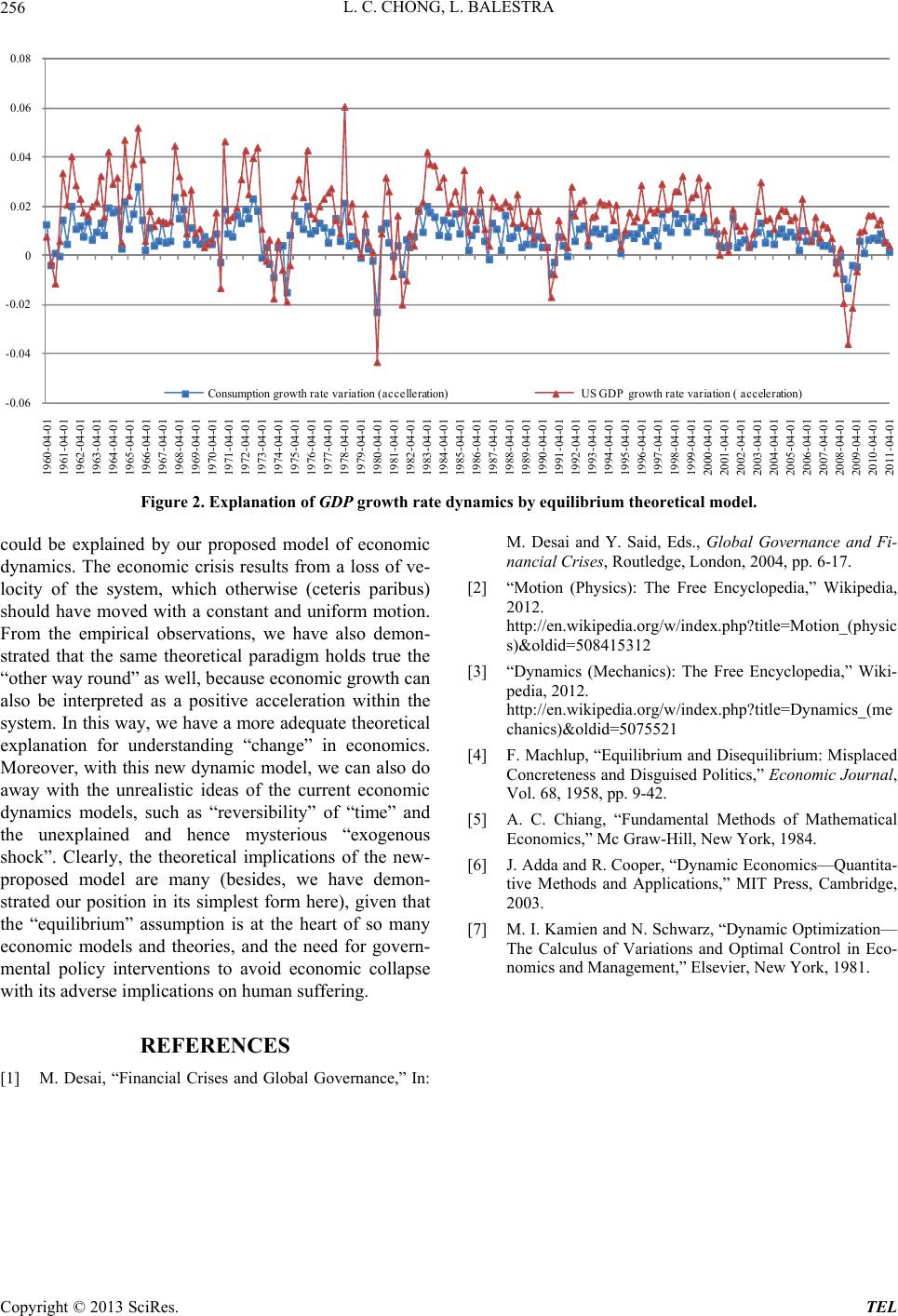

L. C. CHONG, L. BALESTRA

256

-0.06

-0.04

-0.02

0.02

0.04

0.06

0.08

1960-04-01

1961-04-01

1962-04-01

1963-04-01

1964-04-01

1965-04-01

1966-04-01

1967-04-01

1968-04-01

1969-04-01

1970-04-01

1971-04-01

1972-04-01

1973-04-01

1974-04-01

1975-04-01

1976-04-01

1977-04-01

1978-04-01

1979-04-01

1980-04-01

1981-04-01

1982-04-01

1983-04-01

1984-04-01

1985-04-01

1986-04-01

1987-04-01

1988-04-01

1989-04-01

1990-04-01

1991-04-01

1992-04-01

1993-04-01

1994-04-01

1995-04-01

1996-04-01

1997-04-01

1998-04-01

1999-04-01

2000-04-01

2001-04-01

2002-04-01

2003-04-01

2004-04-01

2005-04-01

2006-04-01

2007-04-01

2008-04-01

2009-04-01

2010-04-01

2011-04-01

Consumption growth rate variation (accelleration)US GDP growth rate variation ( acceleration)

Figure 2. Explanation of GDP growth rate dynamics by equilibrium theoretical model.

could be explained by our proposed model of economic

dynamics. The economic crisis results from a loss of ve-

locity of the system, which otherwise (ceteris paribus)

should have moved with a constant and uniform motion.

From the empirical observations, we have also demon-

strated that the same theoretical paradigm holds true the

“other way round” as well, because economic growth can

also be interpreted as a positive acceleration within the

system. In this way, we have a more adequate theoretical

explanation for understanding “change” in economics.

Moreover, with this new dynamic model, we can also do

away with the unrealistic ideas of the current economic

dynamics models, such as “reversibility” of “time” and

the unexplained and hence mysterious “exogenous

shock”. Clearly, the theoretical implications of the new-

proposed model are many (besides, we have demon-

strated our position in its simplest form here), given that

the “equilibrium” assumption is at the heart of so many

economic models and theories, and the need for govern-

mental policy interventions to avoid economic collapse

with its adverse implications on human suffering.

REFERENCES

[1] M. Desai, “Financial Crises and Global Governance,” In:

M. Desai and Y. Said, Eds., Global Governance and Fi-

nancial Crises, Routledge, London, 2004, pp. 6-17.

[2] “Motion (Physics): The Free Encyclopedia,” Wikipedia,

2012.

http://en.wikipedia.org/w/index.php?title=Motion_(physic

s)&oldid=508415312

[3] “Dynamics (Mechanics): The Free Encyclopedia,” Wiki-

pedia, 2012.

http://en.wikipedia.org/w/index.php?title=Dynamics_(me

chanics)&oldid=5075521

[4] F. Machlup, “Equilibrium and Disequilibrium: Misplaced

Concreteness and Disguised Politics,” Economic Journal,

Vol. 68, 1958, pp. 9-42.

[5] A. C. Chiang, “Fundamental Methods of Mathematical

Economics,” Mc Graw-Hill, New York, 1984.

[6] J. Adda and R. Cooper, “Dynamic Economics—Quantita-

tive Methods and Applications,” MIT Press, Cambridge,

2003.

[7] M. I. Kamien and N. Schwarz, “Dynamic Optimization—

The Calculus of Variations and Optimal Control in Eco-

nomics and Management,” Elsevier, New York, 1981.