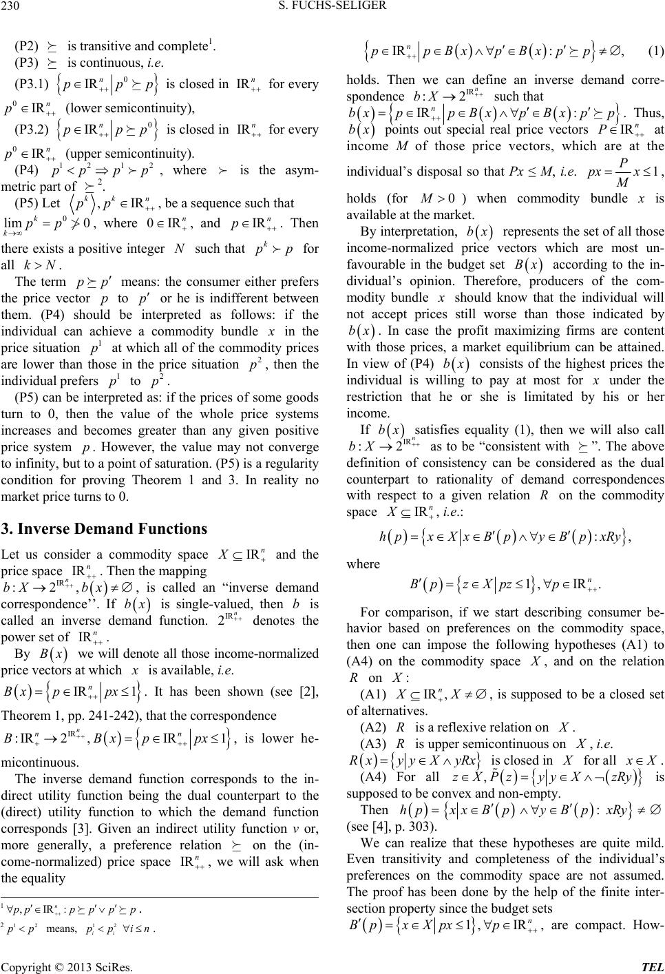
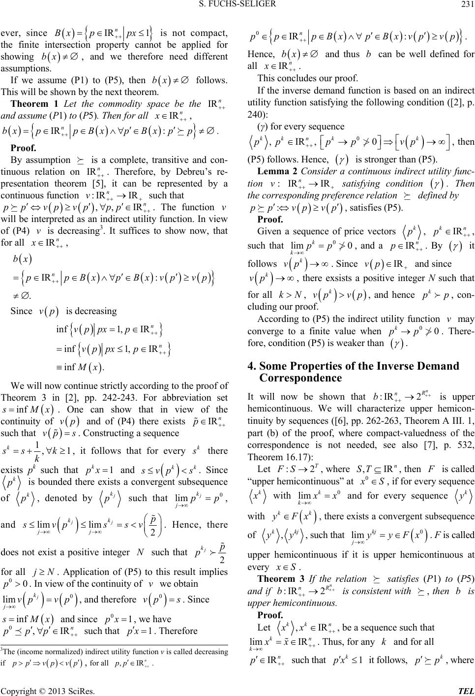
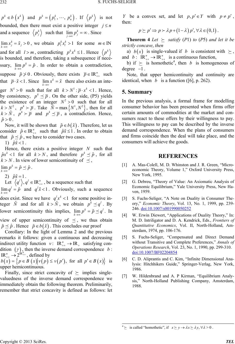
 Theoretical Economics Letters, 2013, 3, 229-232 http://dx.doi.org/10.4236/tel.2013.34039 Published Online August 2013 (http://www.scirp.org/journal/tel) Modelling Consumer Behavior by Inverse Demand Functions Susanne Fuchs-Seliger Institut für Volkswirtschaftslehre Karlsruher Institut für Technologie, Karlsruher, Deutschland Email: susanne.fuchs-seliger@kit.edu Received June 4, 2013; revised July 4, 2013; accepted July 18, 2013 Copyright © 2013 Susanne Fuchs-Seliger. This is an open access article distributed under the Creative Commons Attribution License, which permits unrestricted use, distribution, and reproduction in any medium, provided the original work is properly cited. ABSTRACT In this article a model of consumer behavior will be developed, based on preferences on the price space reflecting the individual’s willingness to pay for certain quantities of commodities under the supposition that the individual is re- stricted to his or her income. Firms offer certain amounts of commodities at the market and consumers react to these offers by their willingness to pay. Existence and continuity of the inverse demand function describing consumer’s be- havior under appropriate conditions will be shown. Furthermore, differences between a model of consumer behavior based on preferences on the commodity space and that which is based on preferences on the price space will be pointed out. Keywords: Consumer Theory; Preference Relation; Inverse Demand Functions; Duality Theory 1. Introduction We will consider inverse demand functions which assign, to every commodity bundle x, those market price com- binations p the individual is willing to pay for x at most when income M prevails. The demand function, defined on prices and income, and the related inverse demand function, defined on commodities offered at the market and on the individual’s income, are dual concepts de- scribing consumer behavior. According to its definition, a demand function associates with every budget set ,BpMxXpx M Inverse demand functions often are a convenient tool for modelling market behavior in the presence of mono- polistic firms ([1], p. 326). If the firms have information about the individual’s preferences on prices, then they will know that he or she cannot accept prices higher than a certain limit. The analysis in this article will be based on preference relations on prices instead of indirect utility functions. Therefore, a more general framework for inverse demand will be established. We will introduce axioms concerning consumer’s preferences on the price space IRn . Based on these axioms properties of the inverse demand func- tion will be deduced. For comparison, we will also point out the difference between a model of consumer behavior based on preferences on the commodity space and that which is based on the price space. , that commodity bundle which according to the preferences of the individual is the one he or she prefers to the other ones available in the given budget set. From the point of duality, according to the individual’s preferences with regard to prices, the inverse demand function points out that price com- bination the individual would spend for x at most, given income . As an example we may consider the fol- lowing one: the individual is not willing to pay more than two Euro for one pound of bred. Then he can afford to buy cheese for not more than three Euro and ham for two Euro. In total the individual cannot spend more than seven Euro for these goods. Evidently, he would be happy if these commodities were cheaper. As another example we can fancy a market where carpets are sold and the agent is not willing to pay more than a certain amount of money for a special carpet. 2. Hypotheses on Consumer’s Preferences Modelling consumer’s behavior we will assume the following hypotheses: (P1) is a relation on the strictly positive n-dimen- sional vector space IR n . Every represents IRn p an income-normalized price vector, i.e. P p , where IRn P are the market prices, i is the price of one unit of the good P i , and M is the income of the indi- vidual, where . 0M C opyright © 2013 SciRes. TEL  S. FUCHS-SELIGER 230 (P2) is transitive and complete1. (P3) is continuous, i.e. (P3.1) 0 IR n pp p is closed in for every IRn 0IRn p (lower semicontinuity), (P3.2) 0 IRn ppp 2 is closed in for every IRn 0IRn p (upper semicontinuity). (P4) , where is the asym- metric part of 2. 12 1 pp pp (P5) Let ,IR kk n pp , be a sequence such that 0 lim 0 k kpp , where 0I, and R n IRn p k . Then there exists a positive integer such that for all . Npp kN The term means: the consumer either prefers the price vector to or he is indifferent between them. (P4) should be interpreted as follows: if the individual can achieve a commodity bundle pp p p in the price situation at which all of the commodity prices are lower than those in the price situation , then the individual prefers to . 1 p 1 p 2 p 2 p (P5) can be interpreted as: if the prices of some goods turn to 0, then the value of the whole price systems increases and becomes greater than any given positive price system . However, the value may not converge to infinity, but to a point of saturation. (P5) is a regularity condition for proving Theorem 1 and 3. In reality no market price turns to 0. p 3. Inverse Demand Functions Let us consider a commodity space and the price space . Then the mapping , is called an “inverse demand correspondence’’. If is single-valued, then is called an inverse demand function. denotes the power set of . IRn X IR 2n IRn , nb IR n IR :2bX x bx Bx b By we will denote all those income-normalized price vectors at which is available, i.e. IR 1 n Bx ppx . It has been shown (see [2], Theorem 1, pp. 241-242), that the correspondence IR : IR2, IR1 n n BBxp n px , is lower he- micontinuous. The inverse demand function corresponds to the in- direct utility function being the dual counterpart to the (direct) utility function to which the demand function corresponds [3]. Given an indirect utility function v or, more generally, a preference relation on the (in- come-normalized) price space , we will ask when the equality IRn IR: , n ppBxpBxpp (1) holds. Then we can define an inverse demand corre- spondence IR : 2n bX such that IRnp B : bxpxpBx pp . Thus, bx points out special real price vectors IRn P at income M of those price vectors, which are at the individual’s disposal so that Px ≤ M, i.e. 1 P px x , holds (for ) when commodity bundle x is available at the market. 0M By interpretation, bx represents the set of all those income-normalized price vectors which are most un- favourable in the budget set according to the in- dividual’s opinion. Therefore, producers of the com- modity bundle Bx should know that the individual will not accept prices still worse than those indicated by bx. In case the profit maximizing firms are content with those prices, a market equilibrium can be attained. In view of (P4) bx consists of the highest prices the individual is willing to pay at most for under the restriction that he or she is limitated by his or her income. If bx IR : satisfies equality (1), then we will also call 2 n bX IR X as to be “consistent with ”. The above definition of consistency can be considered as the dual counterpart to rationality of demand correspondences with respect to a given relation on the commodity space R n , i.e.: : ,hpxXxB pyB pxRy where 1, IR. n Bpz Xpzp For comparison, if we start describing consumer be- havior based on preferences on the commodity space, then one can impose the following hypotheses (A1) to (A4) on the commodity space , and on the relation on R : (A1) , is supposed to be a closed set of alternatives. IR, n XX (A2) is a reflexive relation on R . (A3) is upper semicontinuous on R , i.e. RxyyXyRx is closed in for all X . (A4) For all zRy, zXPz y yX is supposed to be convex and non-empty. Then : hpxxB pyB pxRy (see [4], p. 303). We can realize that these hypotheses are quite mild. Even transitivity and completeness of the individual’s preferences on the commodity space are not assumed. The proof has been done by the help of the finite inter- section property since the budget sets 1,IR: n pppp p . 21 1, IR n Bpx Xpxp , are compact. How- 2 p means, 12 ii pin. Copyright © 2013 SciRes. TEL  S. FUCHS-SELIGER 231 ever, since IR 1 n Bx ppx is not compact, the finite intersection property cannot be applied for showing , and we therefore need different assumptions. bx If we assume (P1) to (P5), then follows. This will be shown by the next theorem. bx Theorem 1 Let the commodity space be the IRn and assume (P1) to (P5). Then for all , IR n x IR : n bxpp BxpBxpp . Proof. By assumption is a complete, transitive and con- tinuous relation on . Therefore, by Debreu’s re- presentation theorem [5], it can be represented by a continuous function such that . The function will be interpreted as an indirect utility function. In view of (P4) is decreasing3. It suffices to show now, that for all , v vp IRn :IRn , , IR IR n pp p pvp v IR n x v IR : . n bx ppBxpBxvpvp Since is decreasing vp inf1, IR inf1, IR inf . n n vp pxp vp pxp Mx We will now continue strictly according to the proof of Theorem 3 in [2], pp. 242-243. For abbreviation set inf Mx. One can show that in view of the continuity of and of (P4) there exists vp IRn p such that . Constructing a sequence svp 1, 1 k ss k k , it follows that for every k there exists pk such that and 1 k px kk vp s . Since k p is bounded there exists a convergent subsequence of k p, denoted by k p such that 0 jpp lim j k , and lim lim2 jj kk jj p svp ssv . Hence, there does not exist a positive integer such that N2 j kp p for all . Application of (P5) to this result implies . In view of the continuity of we obtain jN j k 00pv 0 lim jvp vp , and therefore . Since 0 vp s inf Mx and since 01px , we have 0, Ippp Rn such that . Therefore 1px 0IR : n pppBxpBx vpvp . Hence, bx IRn and thus can be well defined for all b x . This concludes our proof. If the inverse demand function is based on an indirect utility function satisfying the following condition ([2], p. 240): (γ) for every sequence 0 , IR, 0 kk nkk ppp pvp , then (P5) follows. Hence, is stronger than (P5). Lemma 2 Consider a continuous indirect utility func- tion : vIR IR n satisfying condition . Then the corresponding preference relation defined by :p pvpvp , satisfies (P5). Proof. Given a sequence of price vectors k p, IR kn p , such that , and a . By 0 lim 0 k kpp IRn p it follows vp k. Since and since IRvp k vp , there exsists a positive integer N such that for all , kN k vp vp, and hence , con- cluding our proof. k pp According to (P5) the indirect utility function may converge to a finite value when . There- fore, condition (P5) is weaker than v 00 k pp . 4. Some Properties of the Inverse Demand Correspondence It will now be shown that is upper hemicontinuous. We will characterize upper hemicon- tinuity by sequences ([6], pp. 262-263, Theorem A III. 1, part (b) of the proof, where compact-valuedness of the correspondence is not needed, see also [7], p. 532, Theorem 16.17): :IR2 n R n b Let , where , then :2 T FS,IR n ST is called “upper hemicontinuous” at 0 S, if for every sequence k with 0 lim k k x and for every sequence k y with k yFxk , there exists a convergent subsequence of , kkj yy, such that lim j s called upper hemicontinuous if it is upper hemicontinuous at 0kj yyFx . F i every S . Theorem 3 If the relation satisfies (P1) to (P5) an d if :IR2 n R n b is consistent with , then b is upper h Proof. emicontinuous. Let ,IR kkn xx , be a sequence such that lim IR kx kn x n s, for any k and for all . Thu IRp such that 1 k px it flows, k pp 3The (income normalized) indirect utility function v is called decreasing ol , where if pvpvp , for all . , IRn pp Copyright © 2013 SciRes. TEL  S. FUCHS-SELIGER Copyright © 2013 SciRes. TEL 232 k pbx k and k pp p. If 1,, kk n k p is not bounded, thust exist a postegeen there mitive inr jn and a sequence k p such that lim k j p . Since j , we obtain for some lim 0 jj kxx kkk 1 ll px INm and for all ing lm, contradict1 k . Hence k px k p nece e O is bounded, herefore, takinguence if - ssary, lim k pp . In order to obtain a contradiction, and t a subseq k suppos bviously, there exists 0p .IRn p such that 1 . Spxince lim k k x there also exists an inte- ger such that 10N for all 1: 1 k kNpx. Hence, by ccy, onsistenk pp. On th5) yields the existence of an integer 20N such that for all 2 kN, e other side, (P k pp. Take 12 ma ,NNN , then for all x kN , k pp and k pction. Hence, p, a co pbx n that ntradi showTherefore, let us co e exists a positive integer such that 2) 0. Now, it will be p . ˆ1px . I wo nsider ˆIRn p such that n order to obtain that p ve to consider tcases. 1) . ˆ p , we ha 1 ˆ px Hen erce, thN , ˆ px kN. k 1 k for all kN, and therefore ˆ k pp, for all In view ofr semicontinuity o ˆ pp. lowef lim kp ˆ1px . Let, IR ll n qq , be a sequence such that and qu does exist.e hav we thus ob Corollary: In t re ˆ lim kp l q1. Obviously, such a se l qx ence Since we 1 lk qx for some positive in- teger ˆ N and for all k obtain kl pq. By lower micontinuity thplies, lim kl p. In ˆ N , we s im sei kq p view of upper semicontinuity of tain , ud ˆ pp . Hence pbx . This concles our proof of Lemma 2 and the previous he light marks it follows: given a continuous and decreasing indirect utility function v: IRIR n satisfying con- dition , then the inverseespondence b: IR n n , defined by demand corr IR 2 Bx vp ,for alvp lpB x upper hemicontinuous. concavity of implies single- va or bx p is Finally, since strict luedness of the inverse demand crespondence we immediately obtain the following theorem. Preliminarily, remember that strict concavity is defined as follows: let Y be a convex set, and let ,ppY with pp , n: the 0pp p p ,1 . d let it be 1,p P1) to (P5)Theorem 4 Let satisfy ( an n strictly concave, the a) bx is single-valued if nsistent b is cowith , and bIR nn : IR is a continuous function, b) etic4, then b is homogene if is homothous of degree 1 . Note,at th upper hemicontinuitynt 5. Summary analysis, a fo for m REFERE A. Mas-Colell, R. Green y of Value:atic An liger, “A Note on Cons and co rmal frame NCES An Axiom Duality in inuity are odelling , “Micro- alysis of umer The- ide [1] ntical, when b is a function ([6], p. 262). In the previous consumer behavior has been presented when firms offer certain amounts of commodities at the market and con- sumers react to these offers by their willingness to pay. This willingness to pay can be described by the inverse demand correspondence. When the plans of consumers and firms coincide then the deal will take place, and the consumers will achieve the goods. M. D. Whinston and J. economic Theory, Volume 1,” Oxford University Press, New York, 1995. [2] G. Debreu, “Theor Economic Equilibrium,” Yale University Press, New Ha- ven, 1959. [3] S. Fuchs-Se ory,” Economic Theory, Vol. 13, No. 1, 1999, pp. 239- 246. doi:10.1007/s001990050252 [4] W. Erwin Diewert, “Applications of Duality The sated and Direct ory,” In: Demand M. D. Intriligator and D. A. Kendrick, Eds., Frontiers of Quantitative Economics, Vol. II, North-Holland, Am- sterdam, 1974, pp. 106-176. [5] S. Fuchs-Seliger, “Compen without Transitive and Complete Preferences,” Annals of Operations Research, Vol. 23, No. 1, 1990, pp. 299-310. doi:10.1007/BF02204854 [6] C. D. Aliprantis and C. Kim, “Infinite Dime denbrand and A. P Kirman, “Equilibriu 0 nsional Ana- m Analy- lysis: Hitchhikers Guide,” Springer-Verlag, New York, 1986. [7] W. Hil sis,” North-Holland Publishing Company, Amsterdam, 1988. 4 is called “homothetic”, if ,>xyxy .
|