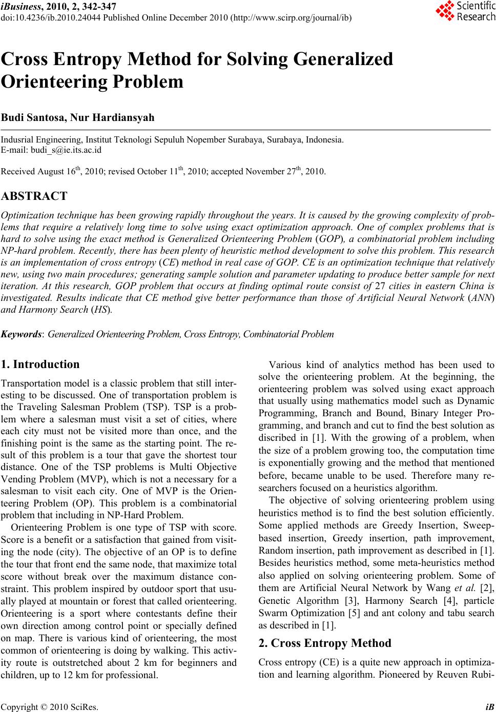iBusiness, 2010, 2, 342-347
doi:10.4236/ib.2010.24044 Published Online December 2010 (http://www.scirp.org/journal/ib)
Cross Entropy Method for Solving Generalized
Orienteering Problem
Budi Santosa, Nur Hardiansyah
Indusrial Engineering, Institut Teknologi Sepuluh Nopember Surabaya, Surabaya, Indonesia.
Received August 16th, 2010; revised October 11th, 2010; accepted November 27th, 2010.
ABSTRACT
Optimization technique has been growing rapidly throughout the years. It is caused by the growing complexity of prob-
lems that require a relatively long time to solve using exact optimization approach. One of complex problems that is
hard to solve using the exact method is Generalized Orienteering Problem (GOP), a combinatorial problem including
NP-hard problem. Recently, there has been plenty of heuristic method development to solve this problem. This research
is an implementation of cross entropy (CE) method in real case of GOP. CE is an optimization technique that relatively
new, using two main procedures; generating sample solution and parameter updating to produce better sample for next
iteration. At this research, GOP problem that occurs at finding optimal route consist of 27 cities in eastern China is
investigated. Results indicate that CE method give better performance than those of Artificial Neural Network (ANN)
and Harmony Search (HS).
Keywords: Generalized Orienteering Problem, Cross Entropy, Combinatorial Problem
1. Introduction
Transportation model is a classic problem that still inter-
esting to be discussed. One of transportation problem is
the Traveling Salesman Problem (TSP). TSP is a prob-
lem where a salesman must visit a set of cities, where
each city must not be visited more than once, and the
finishing point is the same as the starting point. The re-
sult of this problem is a tour that gave the shortest tour
distance. One of the TSP problems is Multi Objective
Vending Problem (MVP), which is not a necessary for a
salesman to visit each city. One of MVP is the Orien-
teering Problem (OP). This problem is a combinatorial
problem that including in NP-Hard Problem.
Orienteering Problem is one type of TSP with score.
Score is a benefit or a satisfaction that gained from visit-
ing the node (city). The objective of an OP is to define
the tour that front end the same node, that maximize total
score without break over the maximum distance con-
straint. This problem inspired by outdoor sport that usu-
ally played at mountain or forest that called orienteering.
Orienteering is a sport where contestants define their
own direction among control point or specially defined
on map. There is various kind of orienteering, the most
common of orienteering is doing by walking. This activ-
ity route is outstretched about 2 km for beginners and
children, up to 12 km for professional.
Various kind of analytics method has been used to
solve the orienteering problem. At the beginning, the
orienteering problem was solved using exact approach
that usually using mathematics model such as Dynamic
Programming, Branch and Bound, Binary Integer Pro-
gramming, and branch and cut to find the best solution as
discribed in [1]. With the growing of a problem, when
the size of a problem growing too, the computation time
is exponentially growing and the method that mentioned
before, became unable to be used. Therefore many re-
searchers focused on a heuristics algorithm.
The objective of solving orienteering problem using
heuristics method is to find the best solution efficiently.
Some applied methods are Greedy Insertion, Sweep-
based insertion, Greedy insertion, path improvement,
Random insertion, path improvement as described in [1].
Besides heuristics method, some meta-heuristics method
also applied on solving orienteering problem. Some of
them are Artificial Neural Network by Wang et al. [2],
Genetic Algorithm [3], Harmony Search [4], particle
Swarm Optimization [5] and ant colony and tabu search
as described in [1].
2. Cross Entropy Method
Cross entropy (CE) is a quite new approach in optimiza-
tion and learning algorithm. Pioneered by Reuven Rubi-

Cross Entropy Method for Solving Generalized Orienteering Problem 343
ensten in 1997, CE method has been used widely in
many problems, such as combinatorial optimization,
continuous optimization, noisy optimization, and rare
event simulation [6]. At these problems, cross entropy
can find optimal or near optimal solution with a less
computational time. The basic idea of the CE method is
to transform the original (combinatorial) optimization
problem to an associated stochastic optimization problem,
and then handling the stochastic problem efficiently by
an adaptive sampling algorithm. Through this process
one constructs a random sequence of solutions which
converges (probabilistically) to the optimal or at least a
reasonable solution. Once the associated stochastic opti-
mization is defined, the CE method follows these two
phases:
1) Generation of a sample of random data (trajectories,
vectors, etc.) according to a specified random mechanism.
2) Update of the parameters of the random mechanism,
on the basis of the data, in order to produce a “better”
sample in the next iteration.
This procedure provides the general frame. When we
are facing a specific problem, like other metaheuristics,
we have to modify CE to fit with our problem. Recently,
CE had been applied in credit risk assessment problems
for commercial banks [7]. Rubinstein used cross entropy
to solve combinatorial and rare-event, estimation [8],
Derek Magee applied cross entropy on a sequential
scheduling approach to combining multiple object classi-
fiers [9], Kroese and Hui used cross entropy in network
reliability estimation [10]. CE application has been
widely adopted in the case of a difficult combinato-
rial such as the maximal cut problem, Traveling Sales-
man Problem (TSP), quadratic assignment problem,
various kinds of scheduling problems and buffer alloca-
tion problem (BAP) for production lines [6].
3.Problem Formulation
Orienteering Problem is one type of TSP with score.
Score is a benefit or a satisfaction that gained from vis-
iting the node (city). The objective of an OP is to define
the tour that front end the same node, that maximize
total score without break over the maximum distance
constraint. This problem inspired by outdoor sport that
usually played at mountain or forest that called orien-
teering. Orienteering is a sport which the contestant
define their own direction among control point or spe-
cially defined on map. There are various kind of an
Orienteering, the most common of an orienteering is
doing by walking. This activity route outstretched about
2 km for a beginner and children, and until 12 km for
professional. This time will be used eastern region of
China as a case.
Figure 1. Map of 27 cities in eastern part of China [4].
If a traveler visits eastern part of China, as shown in
Figure 1 [4], and he/she wants to travel as many cities as
possible with the purpose of best fulfilling multiple fac-
tors such as 1) natural beauty, 2) historical interest, 3)
cultural event, and 4) business opportunities under the
limited total moving distance, his/her travel can become
generalized orienteering problem where each city has
certain quantified scores for all factors and the estimation
of a tour is performed based on the summation of those
scores in the tour. The GOP is a generalization of the
orienteering problem (OP) and the main difference be-
tween the two is that each city in GOP has multiple
scores while each city in OP has only one score. In this
case, Total distance (DMAX) is set to 5000 km.
The objective function of Generalized Orienteering
Problem is maximizing the score of the resulting route as
follows.
1/
1
Max( )
k
mk
gg
giP
ZW Si




 









 (1)
where Wg is the weight of goal g, and the exponent k is
set to 5 in this problem.
Subject to:
1
1
22
1
nn
jin
ji
xx






Cross Entropy Method for Solving Generalized Orienteering Problem 344
11
22
1,2, ,1
nn
ik kj
ij
x
xk n


 
  (2)
11
nn
ij ij
ij
dx DMAX




1, 0
ij
x
,1,,ij n
4. CE Method for GOP
To solve GOP using CE we propose the following
procedure
1) Initialization
Determine α (smoothing parameter), ρ (proportion of
elite sample), N (number of sample), weight (W) of each
criteria in the objective function, maximum distance
allowed and p (initial ttransition matrix). To generate
initial transition matrix with size of n × n, where n is the
number of city, use the following formula
11,.... n
ij i
Pij
n


1,......
1
ij
Pij
n


Each cell in the transition matrix, p(i,j), indicates the
probability of visiting city j from city i. In initial step
each city has the same probability to be visited from
another city.
2) Route Generation
Generate N routes that visit all cities based on the
transition matrix obtained in step 1.
3) Subtour forming
To form subtours, we have to fix the maximum dis-
tance allowed. A route is formed by connecting one city
with other city and so on until the maximum distance is
reached. A city is allowed to be visited once. We use the
following distance formula, where the earth assumed to
be a sphere:
 
1
1
(90 )
,arcsinsinsinsin( )
180
b
dxy rce
 

 



(3)
where
 
12
arctan arctaned d
3 21
1coscos tan
222
c
cc
d 

,
3 21
2sinsin tan
222
c cc
d 


112
180
caa

 ,

221
180
cbb

 ,

312
180
cbb

  
4) Score Calculation
After we have the routes, we can compute the score of
each route by applying Equation (1). The score represents
the fitness. In this case we seek to have maximum score.
5) Elite sample selection
After the score of each route is computed, we chose an
elite sample with size of ρ*N from the whole sample (N).
First, we sort the scores from the highest to the lowest.
Then, we chose the highest score from this elite sample.
Use this elite sample to update the next transition matrix.
By this step a route with maximum score will have
higher probability than other routes.
6) Parameter updating
After we get the elite sample, we calculate the empiri-
cal probability by the following formula:
,
,
ij
ij
n
rN



where ni,j denotes how many times city i and j are
connected in all routes in the generated sample. We then
update the transition matrix using the following formula:




,1
old
pij rp   
where pold is the transition matrix form previous iteration
and r is the empirical probability.
7) Stopping Criteria Checking
If the stopping criteria is met then stop. Otherwise,
repeat steps 3 until 7. One of the stopping criteria
commonly used in CE is the maximum absolute differ-
ence between two consequtive transition matrix. If this
value is less than , then stop.
5. Illustration
To explain how this method works, we give an example
below.
As example for solving the problem using CE, we use
the simple samples, with 5 cities, with 4 scores for each
criteria. For weight, we use W0 = (0.25 0.25 0.25 0.25).
The results will be checked by comparing with the enu-
merative results for validation (Figure 2). There is data
shown in Tables 1 and 2.
Table 1. Distance matrix.
1 2 3 4 5
10.00 106.91 364.05 549.32 264.08
2106.91 0.00 277.33 442.44 263.55
3364.05 277.33 0.00 305.77 269.00
4549.32 442.44 305.77 0.00 562.55
5264.08 263.55 269.00 562.55 0.00

Cross Entropy Method for Solving Generalized Orienteering Problem 345
Table 2. Scores of each node.
No Nama S1 S2 S3 S4
1 Beijing 8 10 10 7
2 Tianjin 6 5 8 8
3 Jinan 7 7 5 6
4 Qingdao 7 4 5 7
5 Shijiazhuang 5 4 5 5
2
5
3
1
4
264.08
269.00
562.55
263.55
106.90
549.32
364.05
277.33
442.44
305.77
Figure 2. Validation node.
1) Initialization
For initialization let α (smoothing parameter) = 0.8, ρ
(proportion of elite sample) = 0.3, N (number of sample
every iteration) = 10, and the weight that used (0.25 0.25
0.25 0.25).
We generate initial transition matrix with size of n × n
where n is the number of city, in this case n = 5, by using
the following formula
11,.... n
ij i
Pij
n


1,......
1
ij
Pij
n


Using this formula we obtain the following transition
matrix:
In this phase we generate routes that visit all cities
based on the transition matrix in Figure 3. The results
are shown in Table 3.
00.25 0.25 0.25 0.25
0.2500.25 0.25 0.25
0.25 0.2500.25 0.25
0.25 0.25 0.2500.25
0.25 0.25 0.25 0.250
p








Figure 3. Transition matrix.
Table 3. Initial routes that generated at iteration 1.
No Route
1 1-4-5-3-2
2 1-3-4-2-5
3 1-4-5-2-3
4 1-3-2-4-5
5 1-4-5-3-2
6 1-2-5-4-3
7 1-2-4-2-5
8 1-3-5-4-2
9 1-3-24-5
10 1-2-5-3-4
2) Subtour
To form subtour, we have to fix the maximum dis-
tance allowed. A subtour is part of route that cut based
on maximum distance, in this example the maximum
distance is set to 1000 km. From Table 3 we obtained
the resulting subtours in Table 4.
Notice that routes number 1, 3 and 5 consist only the
fisrt city. This means that the distance to next visited city
is more than 1000 km.
3) Score Computation
Applying Equation (1) we obtain scores as shown in
Table 5.
Table 4. Resulting subtours.
No Route Distance (km)
1 1 0.00
2 1-3-1 728.11
3 1 0.00
4 1-3-2-1 748.29
5 1 0.00
6 1-2-5-1 634.54
7 1-2-1 213.81
8 1-3-5-1 897.14
9 1-3-2-1 748.29
10 1-2-1 213.81
Table 5. Score of each route.
No Route Score
1 8.75
2 9.16
3 8.75
4 9.72
5 8.75
6 9.50
7 9.42
8 9.25
9 9.72
10 9.42

Cross Entropy Method for Solving Generalized Orienteering Problem 346
00.31670.5833 0.05000.0500
0.050000.0500 0.0500 0.3167
0.31670.583300.0500 0.0500
0.8500 0.0500 0.050000.0500
0.5633 0.0500 0.0500 0.05000
p








4) Elite Sample Selection
Using ρ = 0.3 we have an alite sample of size 3 out of
10. From the score in Table 5 we choose three best
values.
5) Parameter Update
Empirical probability from Elite Sample is shown in
Figure 4.
We then update the transition matrix using the
following formula:
 
,1
old
pij rp   
where pold is (probability matrix from the previous
iteration), in this example is p in Figure 3, and r is
probability matrix in Figure 4 and Table 6. For example
to update p(1,2) with α=0.8 the calculation is as follows:


1, 20.80.3333 10.8 0.250.3167p 
The new p is shown in Figure 5.
Table 6. Elite sample.
No Rute Rute Skor
4 1-3-2-1 9.72
9 1-3-2-1 9.72
6 1-2-5-1 9.50
00.3333 0.6667 00
0000 0.3333
0.3333 0.6667000
10000
0.6667 000 0
p

















Figure 4. Empirical probability matrix.
00.31670.5833 0.0500 0.0500
0.050000.0500 0.0500 0.3167
0.31670.583300.0500 0.0500
0.8500 0.0500 0.050000.0500
0.5633 0.0500 0.0500 0.05000
P

















Figure 5. Updated transition matrice.
6) Stopping Criteria Checking
The stopping crieria used in this experiment is the
maximum absolute difference between two consequtive
transition matrix is less than 0.005.
7) Optimal Route
After doing steps 1 to 8, we found the optimal route as
shown in Table 7. The table also shows the enumerative
result.
Table 7. Result comparison CE-GOP and enumeration.
Method Optimal Route Distance Score
Enumeration 1-2-3-5-1 917.3 9.79
CE-GOP 1-2-3-5-1 917.3 9.79
Table 8. Comparison between CE, HS, and ANN.
Weight Method Distance Score Route
CE 4993.4 12.3793 1-2-3-10-11-12-9-13-17-19-16-20-6-5-1
HS 4993.4 12.3793 1-2-3-10-11-12-9-13-17-19-16-20-6-5-1
W0
ANN 4993.4 12.3793 1-2-3-10-11-12-9-13-17-19-16-20-6-5-1
CE 4946.0 13.1037 1-2-3-8-24-19-16-13-9-12-10-4-27-1
HS 4985.4 13.0825 1-2-3-15-24-19-13-9-12-10-2-27-1 W1
ANN 4987.7 13.0529 1-2-3-4-10-11-12-9-13-16-19-24-20-6-5-1
CE 4974.4 12.5617 1-26-27-3-10-12-9-13-15-20-8-6-5-2-1
HS 4910.6 12.5617 1-26-27-4-10-12-9-13-16-15-20-8-3-2-1 W2
ANN 4875.1 12.5070 1-2-26-27-3-10-11-12-9-13-15-20-6-5-1
CE 4987.5 12.7826 1-2-3-5-6-20-8-15-16-13-9-12-11-10-4-27-1
HS 4987.5 12.7826 1-2-3-5-6-20-8-15-16-13-9-12-11-10-4-27-1 W3
ANN 4987.5 12.7826 1-2-3-5-6-20-8-15-16-13-9-12-11-10-4-27-1
CE 4956.4 12.4273 1-2-3-8-15-16-17-14-12-11-10-4-27-1
HS 4845.2 12.4009 1-2-27-4-10-11-12-14-17-16-15-3-1 W4
ANN 4989.8 12.3616 1-2-3-10-9-13-16-17-14-12-11-4-27-1

Cross Entropy Method for Solving Generalized Orienteering Problem 347
6. Experiments and Analysis
We show the results of numerical experiments and the
comparison with those of other methods in Table 8.
There are five set of different weight vectors used in the
experiments. These weights were applied on three
methods. The values of the weight vectors are W0 =
(0.25, 0.25, 0.25, 0.25), W1 = (1, 0, 0, 0), W2 = (0, 1, 0,
0), W3 = (0, 0, 1, 0), and W4 = (0, 0, 0, 1). W0 = (0.25,
0.25, 0.25, 0.25), means that each criteria has the same
weight. By W1 = (1, 0, 0, 0), we means that only natural
beauty is considered. The similar meaning is for W2, W3
and W4. The last three weight vectors stress only one
goal and ignore the other three. For W0 and W3, we see
that all three methods produce the same routes as well as
the score. For W1 and W4, CE produced the best result
in terms of score.
For W2, CE and HS produced the same results in
terms of score with different Distance and routes. As we
know, distance is limited by maximum value of 5000 km.
7. Conclusions
In this paper we show how Cross Entropy can be applied
for solving Generalized Orienteering Problem whose
objective is to find the best tour in eastern part of China.
The main steps of CE consist of: generate sample, select
elite sample with best fitness, update parameters based
on the elite sample, generate next better sample using the
updated parameters. This procedure can be succesfully
translated for GOP. Generally Cross Entropy shows
equal or solution compared to those of Harmony Search
and Artificial Neural Network.
REFERENCES
[1] Z. Sevkli, and F. dan Erdogan Sevilgen, “Variable Neigh-
borhood Search for the Orienteering Problem,” A. Levi et al.,
Eds., ISCIS, Springer-Verlag, Berlin, Heidelberg, 2006,
pp. 134-143.
[2] Q. Wang, X. Sun, B. L. Golden and J. Jia, “Using Artifi-
cial Neural Networks to Solve the Orienteering Problem,”
Annals of Operations Research, Vol. 61, No. 1, 1995, pp.
111-120.
[3] Tasgetiren and M. Fatih, “A Genetic Algorithm with an
Adaptive Penalty Function for Orienteering Problem,”
Journal of Economic and Social Research, Vol. 4, No. 2,
2000, pp. 1-26.
[4] G. Z. Woo, T. C. Li, D. Park and J. Yong, “Harmony
Search for Generalized Orienteering Problem: Best
Touring in China,” L. Wang, K. Chen and Y. S. Ong,
Eds., Springer-Verlag, Berlin Heidelberg, 2005, pp. 741-
750.
[5] Z. Sevkli and F. dan E. Sevilgen, “Particle Swarm
Optimization for the Orienteering Problem,” Proceedings
of International Symposium on Innovation in Intelligent
Systems and Applications, Istanbul, 2007, pp. 185-190.
[6] R. Rubinstein and D. Kroese, “The Cross-Entropy
Method: A Unified Approach to Combinatorial Optimi-
zation,” Monte-Carlo Simulation, and Machine-Learning,
Springer-Verlag, Berlin, Heidelberg, 2004.
[7] H. Zhou, J. Wang and Y. Qiu, “Application of the Cross
Entropy Method to the Credit Risk Assessment in an
Early Warning System,” International Symposiums on
Information Processing, 2008.
[8] R. Y. Rubinstein, “Stochastic Minimum Cross-Entropy
Method for Combinatorial Optimization and Rare-Event
Estimation,” Methodology and Computing in Applied
Probability, Vol. 7, No. 1, 2005, pp. 5-50.
[9] D. Magee, “A Sequential Scheduling Approach to Com-
bining Multiple Object Classifiers Using Cross-Entropy,”
T. Windeatt and F. Roli, Eds., Springer-Verlag, Berlin,
Heidelberg, 2003, pp. 135-145.
[10] D. P. Kroese and K.-P. Hui, “Applications of the Cross-
Entropy Method in Reliability,” Computational Intelli-
gence in Reliability Engineering, Vol. 40, 2007, pp. 37-
82.