 Open Journal of Applied Sciences, 2013, 3, 285-292 doi:10.4236/ojapps.2013.33036 Published Online July 2013 (http://www.scirp.org/journal/ojapps) Neural Network Approach for Solving Singular Convex Optimization with Bounded Variables* Rendong Ge#, Lijun Liu, Yi Xu School of Science, Dalian Nationalities University, Dalian, China Email: #bgrbgg@163.com, liulijun@dlnu.edu.cn, xuyi@dlnu.edu.cn Received May 1, 2013; revised June 1, 2013; accepted June 8, 2013 Copyright © 2013 Rendong Ge et al. This is an open access article distributed under the Creative Commons Attribution License, which permits unrestricted use, distribution, and reproduction in any medium, provided the original work is properly cited. ABSTRACT Although frequently encountered in many practical applications, singular nonlinear optimization has been always rec- ognized as a difficult problem. In the last decades, classical numerical techniques have been proposed to deal with the singular problem. However, the issue of numerical instability and h igh computational complexity ha s not found a satis- factory solution so far. In this paper, we consider the singular optimization problem with bounded variables constraint rather than the common unconstraint model. A novel neural network model was proposed for solving the problem of singular convex optimization with bounded variables. Under the assumption of rank one defect, the original difficult problem is transformed into nonsingular constrained optimization problem by enforcing a tensor term. By using the augmented Lagrangian method and the projection technique, it is proven that the proposed continuous model is conver- gent to the solution of the singular optimization problem. Numerical simulation further confirmed the effectiveness of the propos ed neural n etwork approach. Keywords: Neural Networ ks; Singular Nonlinear Optim i zat i on; Stati o nar y Point; Augmented Lagrangian Fu nct ion; Convergence; LaSalle’s Invariance Principle Plain 1. Introduction The nonlinear model with rank one defect is of great importance for its singular nature. Follwing works of Schnabel and Dan Feng [1-3], we have made great im- provement for such problem by applying Tensor methods by numerical solution [4,5]. For large-scale computational problems, the computation of the classical numerical method is still far from satisfactory. In recent years, neural network approaches were proposed to deal with classical nonlinear optimization problems. Xia and Wang [6] presented neural networks for solving nonlinear convex optimization with bounded constraints and box constraints, respectively. Xia [7,8], Xia and Wang [9,10] developed several neural networks for solving linear and quadratic convex programming problems, monotone linear complementary problems, and a class of monotone variational inequality problems. Recently, projection neural networks for solving mono- tone variational inequality problems are developed in [11-13] and recurrent neural networks for solving nonconvex optimization problem have been also studied [14,15]. It is regrettable that the study of singular non- linear optimization problems in the neural network me- thod have not been involved . Recently, more attention were paid to the singular optimization problems due to real applications. For example, in the problem of singular optimal control, assume the state equation is depicted as d,, d x xut t where is an -dimensional state vector and is an -dimensional control vector, and the control piecewise functions satisfy that n u m,1,2,, jj uMj m . The cost functional is given as 0 ,, f t ff t,d xttLxut t for which the Hamiltonian function is T ,,,, . L xutFxut *Supported by National Natural Science Foundation of China (No. 61002039) and The Fundamental Research Funds for the Central Uni- versities (No. DC10040121 and DC12010216). #Corresponding author. According to the maximum’s principle, when the control variables change in the constrain boundary, the Copyright © 2013 SciRes. OJAppS  R. D. GE ET AL. 286 minimum conditions of the optimal control function are derived as 2 2 0, 0 HH uu If on a given time interval 12 0 ,, f tt tt , there exists that 2 2 det 0 H u , then this becomes the so- called singular optimal control problem. The optimal trajectory corresponding to the segment called singular arc. The numerical methods for solving such singular control problem can be referred to [16,17]. Due to the inherent Parallel mechanism and high- speed of hardware implementations, efforts to tackle such problems by using neural systems are promising and creative. Attempt was made for the first time in our recent paper [18] to solve unconstraint singular optimiza- tion problem, which turned out to be feasible and effect- tive. In this paper, we further improve such result to the case of singular optimization problem with bounded variables constraint. This paper is organized as follows. In Section 2, the nonlinear singular convex optimization problem and its equivalent formulations are described. In Section 3, a recurrent neural network model is proposed to solve such singular nonlinear optimization problems. Global con- vergence of the proposed neural network is analyzed. Finally, in Section 4, several illustrative examples are presented to evaluate the effectiveness of the proposed neural network method. 2. Problem Formulation and Neural Design Let n Rlx h . Assume :, xR is a continuous differentiable convex function. Consider the following unconstrained co nv ex pro gram ming problem, min s.t. fx lxh (1) which can be easily transformed to equivalent non- negative bounded convex programming problem by using the such transformation as , uxl min s.t. 0. fx c (2) Let is the unique optimal solution to (2). We will discuss the solution of (2) under the following as- sumptions. Assumption 1 x is both strictly convex and four times continuous differentiable. For optimum point , 1 there exists such that and . n v vR 2f x 2 rankf xn Null Assumption 2 For x , there exists T2 0ufxu o n uR. Moreoverfor any nonzer, 2 x and 3 x are all unly bounded. iform Assumption 3 For any , the quantity 2 vNull fx T22 0.fxv fxvv 44 v v (The reason for this assumption can be found, for example, in [4].) Lemma 1 For any and n pRT0pv , , 2 vNull fx 2T xpp is nonsingular at . Proof. It is easy to verify this result, thus its proof is omitted here for the sake of saving space. It is seen that when in Lemma 2.1 take random values, the condition is satisfied with pro- bability 1. p T pv 0 Define function x as follows , xfx hx where 2 hxf xx x , 1 2T fx ppp where T0pv . According to the definition of x, we have the following important result, Lemma 2 For any 0 , the Hessian matrix 2 x is positive definite. Moreover, if is small enough, then 2 x is positive definite for any n R. Proof. This conclusion can be proved easily according to the results in [4] under Assumption A2 . Thus the proof is omitted here. Because the Hessian matrix of x is singular at for (2), it is generally difficult to obtain ideal con- vergence results by conventional optimization algorithm (see [1-4]). In order to overcome this difficulty, alter- natively we deal with equivalent unconstrained convex optimization problem as follows, 0 , Fxmin s.t. c (3) for which we can establish the equivalent lemma as fol- lows, Lemma 3 is a solution o f (2) if an d only if is a solution of (3). Further consider the difficulty caused by computing the matrix inverse, we turn optimization questio n (3) into the following equivalent constrained optimization pro- blem. T2 2T min s.t.0 . , xyfxyf xy xppypxc (4) Copyright © 2013 SciRes. OJAppS  R. D. GE ET AL. 287 Define La gr ange fun ction of (4) as follows, T2 T2 T ,,Lxyzf xyf xy zfxppy p By Assumptions A2 and Lemma 2, it is easy to know that the function , xy is strictly convex. And based on the Karush-Kuhn-Tucker sufficient conditions, the KKT point ˆˆ , y of the formula (4) is a unique optimal solution of the optimization question (4) and there exits satisfies the following condition: ˆn zR 0, if0, ,,0,if,1,2, , 0,if 0,. ,, 0, ,, 0, 0 i xii i ii y z n x Lxyzx cin xc Lxyz Lxyz xxRxc Equivalently, the point ˆˆˆ ,, yz satisfies the fol- lowing condition, T ˆˆ ˆˆ ,, 0, ˆˆˆ ,, 0, ˆˆˆ ,, 0. x y z xx Lxyzx Lxyz Lxyz (5) In order to discuss the constrained programming pro- blem (4), first, we define a augmented Lagrangian func- tion of (4) as follows T2 T2 T 2 2T ,,, ,, 2 Lxyzkf xyf xy zfxppyp kfxppy px where is a penalty parameter and is an approximation of the Lagrange multiplier vector. Hence, the problem (4) can be solved by the stationary point of the following problem, 0kz ,, min,, , n xyzR Lxyzk (6) Then, the condition (5) can be written as T ˆˆˆ ˆ ,,, 0,, ˆˆˆ ,,, 0, ˆˆˆ ,,, 0. x y z xx Lxyzkx Lxyzk Lxyzk (7) Now, we introduce the projection function P as follows, 12 ,,,, nn RPuPuPuP where u , i 0, 0, ,0, ,. i iii iii u Pu uuc cuc (8) From the projection conclusion as shown in [19], the first inequality of (7) can be equivalently represented as ˆˆˆˆ ˆ ,,,0, 0. x PxLxyzk x So the optimal solution of (4) and the stationary point of (6) meet with the conditions 2T ,,, ,0, ,,, 0, . x y x xPx Lxyzk Lxyzk fxpp yp (9) 3. Stability Analysis of the Neural Network Model By Theorem 8 and Theorem 9 in [20], there exists a constant , such that if is an optimal solution of the problem (6), then 0k ,,cxyz , y is an optimal solution of the problem (4) and ,, min,, ,. n xyzR Lxyzkf x Notice that ,, ,,,LxyzLxyzk . By the Lagrange function defined above, we can describe the neural network model by the following nonlinear dynamic system for solving (10). The logical graph is shown in Figure 1. 33 32T 22T 2T2T 2T d,, d d,, d 2 d,, d ,1,2,, ,1,2,, jj kk xPxxLxyz x t P xfxfxyyfxyz kfxyfxppyp x vyLx y z t fxyfxpp z k fxppfxppyp wzLx yzfxppyp t ysvj n zswkn (10) w here Copyright © 2013 SciRes. OJAppS  R. D. GE ET AL. Copyright © 2013 SciRes. OJAppS 288 Figure 1. Logical graph of the proposed neural network model. 0 , T 12 ,,, ,0, n fxfx f xf x T 322 2 12 ,,, n xyf xyfxyfxy d,, , d x Px xLxyz t we have 00 ded e, and the activation function is continuou sly differentiable and satisfies that 0s. It is easy to see that if c ,xy , z , then it is a equ is an optimal solution of the problem (6)ilibrium point of network (10). Conversely, if ,, yz is a equilibrium point of network (10), it m point of original problem (4). To analyze the convergence of the neural network (10), the following lemmas are first introduced (see [19]). Lemma 4 Assume n ust be KKT that the set is a closed co aliti R nvex set, then the following two ineques hold, T0, , n PxyxPxx Ry ,, n Px Pyx yxyR where is a projection operator defined as :n PR minP For any inal poi . Lemma 5itint 3 00 0 ,, n tvtwt R, there exists a unique continuous solution 3 ,, n t t of (1 vtwtR for (10). Moreover, xt pro . The equilibrium poin0) solves (5). Proof: By Assumption A1, P vided that 0 xt ,,, x xLxyzk x , ,,, yLxyzk and 2T xppyp are lo According to local cally Lipschitz continuous. existence theorem of ordinary differential equation, there exists a unique continuous solution ,, tvtwt of (10) for 0,tT. Next, let initial point 0 xt . Since , d d tt ss tt x sPxxLxzs t ently, . y Or equival 0 0 0 eee ,, t tt ts td txt PxxLxyz s So, 0xt provided that 00xt , ,,, 0Px yzk xLx t ts , and since 0 0 0 0 0 eee ,, e ee e tt tt tt tt 0 0 0 e t t d txt PxxLxyz xt ccxt c s . Thus, c xt re establishin provided that Befog the convergem, we need the property of the following augmented Lagrangian fu 0 xt . nce theore nction. Assumption 4 ,,Lxyz satisfies the local mono- tone property of following definition about . T,, x Lxyz Lxyz , ,0. x xx Now we are ready to establish the stability and the convergence res ults of network (10). Theorem 6 Assume that :n xR R is strictly convex and the fourth differentiable, and ,,cxyz is a global optimal solution of the problem (6), if the initial point 00 ,, 0 tytzt  R. D. GE ET AL. 289 with 0 xt is chosen in a small neighborhood of point, then the proposed neural network of (10) is stable in the sense of Lyap convehe stationary point ,, the equunov and globally ilibrium rgent to t yz , where is the optimal solution of (2). Proof. We define V: R as follows: 2, 2 zfx show that is a suitable Lypov cmic system (10), it is evident that ,,Vxtytzt 1 ,,Lxt yttxtx W fun e want to tion for dynaVun 2 1 ,, , 2 Vxtytztxtx , ,, ,, tytzt xyz ,, 0.Vx yz Then 1 1 T T dd ddd ,, ddddd ddddd ,, . niii iii x niiiii iiiiii x xy VLL L utytzt xxPxLxyzx dz d d i t And denote that 12 ,,, vn Gdiagsvsv sv , 12 ,,, wn Gdiagswsw sw we have yv zw LL L tyvtzwt xxPxLxyzx (11) 1 T T T T T T T dd d dd d ,, dd ,, ,, dd d ,, d ,, ,, ,, nii ii iii i x xyv zw x xx d d i vw VLL L sv sw t xtytzt xxPxLxyzx xv LxyzLxyz G tt w LxyzGt xxPxLxyzx LxyzP xLxyzx xx T T ,, ,, ,, ,,,, . x yvy zwz PxLxyz x Lxyz G Lxyz LxyzGLxyz (12) In the first inequality of Lemma 4, let ,, x xLxy z and x , then C T ,,,,,, 0. xxx Px Lxyzxx LxyzPx Lxyz onsequently, T T 2 T ,, ,, ,, ,, ,, . xx x x x PxLxyz xLxyz Px Lxyz xaxx Lxyz xx xPxLxyz (13) Then, we o b t ain from (12), (1 3 ) and Assumption A 4 2 T T ,, ,, ,, ,, ,, ,, ,, 0, x yv y zwz VxyzP xLxyzx xx Lxyz Lxyz G Lxyz LxyzG Lxyz (14) T dx t d d,,0 d Vxyz t (15) consequently, ,,VPxtytzt by (14), it is evident th is Lypunov function, and at dddd 00,0,0. tdddd Vxvw ttt By the Lypunov stability theory, systems (10) is le. Therefore, when ti asymptotically stabhe intial point 000 ,, yx is obtain near to the equilibrium point, the set 0 ,, tytzttt is bounded. By also using nvariant principle, the trajectory of the neural LaSall's i network (10) ,,ut yt zt will converge to the ximum invariant subset of the following set ma d ,, 0. d V ExyzS t Assume again that ,, xxyz E , then we have lim, 0. tdistx tX x , we have Specially, when . t lim tx Copyright © 2013 SciRes. OJAppS 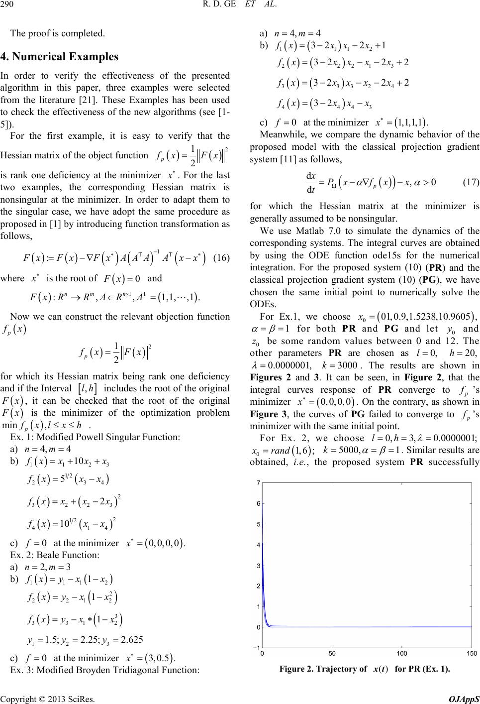 R. D. GE ET AL. 290 The proof is completed. 4. Numerical Examples In order to verify the effectiveness of the presented algorithm in this paper, three examples were selected frese Examples has been used e new algorithms (see [1- om the literature [21]. Th to check the effectiveness of th 5]). For the first example, it is easy to verify that the Hessian matrix of the object function 2 1 2 p xFx is rank one deficiency at the minimizer . For the last two examples, the corresponding matrix is no e procedure as n transformation as Hessian nsingular at the minimizer. In order to adapt them to the singular case, we have adopt the sam proposed in [1] by introducing functio follows, 1 TT : xFx FxAAAAxx (16) where is the root of 0Fx and 1Tnm n FxRRA RA :,,1,1, ,1. Now we can construct the relevant objection function p x 2 1 2 p xFx fo an if r which its Hessian matrix being rank one deficiency dthe Interval ,lh includes the root of the original x , it can be hat the root of the original checked t x min p is the mif the opization problem nimizer otim , xl xh . Ex. 1: Modified Powell Singular Function: a) 4, 4nm 1123 10 b) xx xx 12 34 5 2 xxx 2 3223 2 xx xx 2 12 41 10 4 xxx c) at the minimizer Ex. e Function: a) b) 2 0f 2: Beal 0,0,0,0 .x 2, 3nm 111 1 xyx x 2 21 2 12 xyx x 1 1 2 3 33 xyxx 12 3 1.5;2.25; 2.625yy y c) at the minimizer Ex. fied Broyden Triion: a) 0f 3: Modi 3,0.5 .x diagonal Funct 4, 4nm b) 111 3221fxxxx 2 2221 32 2fxxxxx 3 2 33324 322 2fxxxxx 44 32 43 xxxx c) 0f Meanwhile, we com at the minimizer pare thevior of the proposed model with the classical prection gradient system [11] as follows, 1,1,1 .x dynamic beha 1, oj dPx f t d,0 p xxx (17) simulate the dynamics of the corresponding systems. The integral curves a by using the ODE function ode15s for the numerical ch for which the Hessian matrix at the minimizer is generally assumed to be nonsingular. We use Matlab 7.0 tore obtained integration. For the proposed system (10) (PR) and the classical projection gradient system (10) (PG), we have osen the same initial point to numerically solve the ODEs. For Ex.1, we choose 001,0.9,1.5238,10.9605 ,x 1 for both PR and PG and let 0 y and 0 z be some random values between 0 and 12. The other parameters PR are chosen as 0,l 20,h 0.0000001, 3000k . The results are shown in Figures 2 and 3. It can b urves response of PR converge to e seen, in Figure 2, that the integral c ’s nimizer mi 0,0,0,0x. On the contrary, as shown in Figure 3, the curves of PG failed to converge to ’s in miniitial point. For Ex. 2, we choose 0, 3,0.0000001;lh mizer with the same 01, 6;xrand 5000, 1k . Similar results are obtained, i.e., tsed system PR successfully he propo Figure 2. Trajectory offor PR (Ex. 1). ()xt Copyright © 2013 SciRes. OJAppS 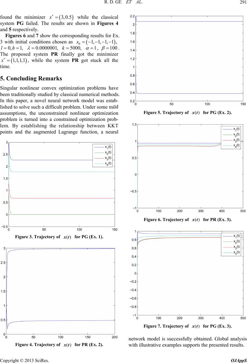 R. D. GE ET AL. 291 found the minimizer while the classical system PG failed. Thshown in Figures 4 and 5 respectively. Figures 6 and 7 show the corresponding results for Ex. 3 with initial conditions chosen as 3,0.5x e results are 01,1, 1, 1,x 0, 1,lh 0.0000001, 50k00, 1 , 100 . got the minimizer PR got stuck all the The proposed 1,1,1,1x time. system PR , while the sy finally stem 5. Concluding Remarks Singular nonlinear convex optimization problems have been traditionally studied by classical numerical methods. In this paper, a novel neural network model was estab lished to solve such a difficult problem. Under some mil assumped nn constraine mented Lagrange function, a neural - d tions, the unconstrainonlinear optimizatio problem is turned into a d optimization prob- lem. By establishing the relationship between KKT points and the aug Figure 3. Trajectory of ()xt for PG (Ex. 1). Figure 4. Trajectory of for PR (Ex. 2). ()xt Figure 5. Trajectory of for PG (Ex. 2). ()xt Figure 6. Trajectory offor PR (Ex. 3). ()xt Figure 7. Trajectory of for PG (Ex. 3). ()xt network model is successfully obtained. Global analysis with illustrative examples supports the presented results. Copyright © 2013 SciRes. OJAppS  R. D. GE ET AL. Copyright © 2013 SciRes. OJAppS 292 REFERENCES [1] R. B. Schnabel and T.-T. Chow, “Tensor Methods for Unconstrained Optimization Using Second Derivativ SIAM: SIAM Journal on Optimization, Vol. 1, No. 3, 199 1, pp. 293-315. doi:10.1137/0801020 es,” [2] D. Feng and R. B. Schnabel, “Tensor Methods for Equ lity Constrained Optimization,” SIAM: SIAM Journal on Optimization, Vol. 6, No. 3, 1996, pp. 653-673. doi:10.1137/S1052623494270790 a- [3] A. Bouaricha, “Tensor Methods for Large Sparse Uncon- strained Optimization,” SIAM: SIAM Journal on Optimi- zation, Vol. 7, No. 3, 1997, pp. 732-756. doi:10.1137/S1052623494267723 [4] R. Ge and Z. Xia, “Solving a Type of Modified BFGS Algorithm with Any Rank Defects and the Local Q-S perliner Convergence Properties,” Journal of Computa- tioatics , 2006 pp. 193-208. Advances and Applications, pp. 17- 35. u , - nal and Applied Mathem, Vol. 22, No. 1-2 [5] R. Ge and Z. Xia, “A Type of Modified BFGS Algorithm with Rank Defects and Its Global Convergence in Convex Minimization,” Journal of Pure and Applied Mathematics: , Vol. 3, No. 1, 2010 [6] Y. S. Xia and J. Wang, “On the Stability of Globally Pro- jected Dynamical Systems,” Journal of Optimization Theory and Applications, Vol. 106, No. 1, 2000, pp. 129- 150. doi:10.1023/A:1004611224835 [7] Y. S. Xia and J. Wang, “A New Neura l Network for Solv- ing Linear Programming Problems and Its Applications,” IEEE Transactions on Neural Networks, Vol. 7, No. 2, 1996, pp. 525-529. doi:10.1109/72.485686 [8] Y. S. Xia, “A New Neural Network for Solving Linear and Quadratic Programming Problems,” IEEE Transac- tions on Neural Networks, Vol. 7, No. 6, 1996, pp. 1544- 1547. doi:10.1109/72.548188 [9] Y. S. Xia, J. Wang, “A General Methodology for De- signing Globally Convergent Optimization Neural Net- works,” IEEE Transactions on Neural Networks, Vol. 9, No. 6, 1998, pp. 1331-1343. doi:10.1109/72.728383 [10] Y. S. Xia, “A Recurrent Ne ural Network for Solving Lin- ear Projection Equations,” IEEE Transactions on Neural Networks Vol. 13, No. 3, 2000, pp. 337-350. doi:10.1016/S0893-6080(00)00019-8 [11] Y. S. Xia, H. Leung and J. Wang, “A Projection Neural Network and Its Application to Constrained Optimi 58. zation Problems,” IEEE Transactions on Circuits and Systems I, Vol. 49, No. 4, 2002, pp. 447-4 doi:10.1109/81.995659 [12] Y. S. Xia and J. Wang, “A General Projection Neural Network for Solving Monotone Variational Inequality and Related Optimization Problems,” IEEE Transactions on Neural Networks, Vol. 15, No. 2, 2004, pp. 318-328. doi:10.1109/TNN.2004.824252 [13] X. Gao, L. Z. Liao and W. Xue, “A Neural Ne Class of Convex Quadratic Minimax Ptwork for a roblems with Con- straints,” IEEE Transactions on Neural Networks, Vol. 15, No. 3, 2004, pp. 622-628. doi:10.1109/TNN.2004.824405 [14] C. Y. Sun and C. B. Feng, “Neural Networks for Non- convex Nonlinear Programming Pro Control Approach,” Lecblems: A Switching ture Notes in Computer Science, Vol. 3496, 2005, pp. 694-699. doi:10.1007/11427391_111 [15] Q. Tao, X. Liu and M. S. Xue, “A Dynamic Genetic Al- gorithm Based on Continuous Neural Networks for a Kind of Non-Convex Optimiza tion Problems,” Applied Mathematics and Computation, Vol. 150, No. 3, 2004, pp. 811-820. doi:10.1016/S0096-3003(03)00309-6 [16] D. J. Bell and D. H. Jacobson, “Singular Optimal Control Problems,” Academic Press, New York, 1975. [17] F. Lamnabhi-Lagarrigue and G. Stefani, “Singular Opti- mal Control Problem: On the Necessary Conditions of Optimality,” SIAM: SIAM Journal on Control and Opti- mization, Vol. 28, No. 4, 1990, pp. 823-840. doi:10.1137/0328047 [18] L. Liu, R. Ge and P. Gao, “A Novel Neural Network for Solving Singular Nonlinear Convex Optimization Prob- lems,” Lecture Notes in Computer Science, Vol. 7063, 2011, pp. 554-561. doi:10.1007/978-3-642-24958-7_64 [19] D. Kinderlehrer and G. Stampacchia, “An Introduction to w and K. E. Hillstrom, “Testing Variational Inequalities and Their Applications,” Aca- demic Press, New York, 1980. [20] X. Du, Y. Yang and M. Li, “F urther Studies on the Heste- nes-Powell augmented Lagrangian Function for Equality Constraints in Nonlinear Programming Problems,” OR Transactions, Vol. 10, No. 1, 2006, pp. 38-46. [21] J. J. More, B. S. Garbo Unconstrained Optimization Software,” ACM Transac- tions on Mathematical Software, Vol. 7, No. 1, 1981, pp. 19-31. doi:10.1145/355934.355936
|