International Journal of Geosciences, 2013, 4, 898-903
http://dx.doi.org/10.4236/ijg.2013.45084 Published Online July 2013 (http://www.scirp.org/journal/ijg)
A Novel Approach in Identification of Urban Hot Spot
Using Geospatial Technology: A Case Study in Kamrup
Metro Distric t o f Assam
Jonali Goswami, Shreya Roy, S. Sudhakar
Department of Space, North Eastern Space Applications Centre, Umiam, India
Email: Jonali.goswami@gmail.com, hi_rumpa@yahoo.co.in, s.sudhakar@nesac.gov.in
Received April 19, 2013; revised May 22, 2013; accepted June 20, 2013
Copyright © 2013 Jonali Goswami et al. This is an open access article distributed under the Creative Commons Attribution License,
which permits unrestricted use, distribution, and reproduction in any medium, provided the original work is properly cited.
ABSTRACT
Urbanization in recent years plays an important role in increase in impervious areas with reducing in vegetation cover
and pervious areas of natural landscape. This leads to a rise in temperature of urban areas, by several degrees particu-
larly at night [1,2]. A novel geospatial approach has been adopted to determine the maximum temperature areas (hot
spots) over Kamrup Metro District of Assam, which is a gateway for seven neighboring north eastern states of India.
The G statistics have been calculated for detecting the presence of hot spot or cold spot over the entire study area which
is a new approach in urban heat island studies. The resultant z-scores and p-values show the pixels with either high or
low values cluster spatially. For statistically significant positive z-scores, the larger the z-score is, the more intense the
clustering of high values (hot spot) and vice versa. Land Surface Temperature (LST) anomaly values and percentage of
Impervious Surface Area (ISA) along with climatic data are used to conform the hot spot location. It is one of the
densely populated areas with more commercial pockets thereby giving rise to anthropogenic heat discharge which ac-
celerates the heat island phenomenon. Incorporation of socio-economic survey data as well as certain biophysical pa-
rameters can be used to know about the cause and future impact of urbanization.
Keywords: Hot Spot; LST; G Statistics; Impervious Area; Geospatial; RS GIS
1. Introduction
Vegetation cover has been replaced by impervious areas
in most parts of the world in recent years thus giving rise
to urban heat island, in which the temperature of urban
areas is several degrees higher than non urbanized areas
surrounding them, particularly at night [1,2]. The imper-
vious areas is largely contributed by use of materials like
concrete, bricks, tiles etc. for buildings and bitumen for
roads and parking lots [3]. The introduction of new sur-
face materials coupled with emission of heat, moisture
and pollutants dramatically change radiative, thermal,
moisture, roughness and emission properties of the sur-
face and the atmosphere above [4]. The effect of this can
be analyzed by observing the variation of night time LST
over different land use classes within the study area. LST
is generally defined as the skin temperature of the surface
which refers to land temperature for bare soil, canopy
surface temperature for densely vegetated ground and
combination of two in case of sparsely vegetated ground.
Satellite derived LST has been used for a number of ur-
ban hot spot analysis where LST dynamics with bio-
physical properties has been studied [5-7]. Past studies
explain the fact that green areas provide a cooling effect
to the surroundings in a city and the increase in building
spaces leads to a rise in LST.
Another indicator of urban hot spot is the percent im-
pervious area (%ISA) which bears a strong linear rela-
tionship with the LST [8]. The amount of impervious
surfaces is related to population growth and urbanization
[3]. The first global grid of %ISA at one km grid has
been prepared by Earth Observation Group, NOAA Na-
tional Geophysical Data Center, based on two coarse
resolution indicators of ISA—the brightness of satellite
observed nighttime lights and population count.
The main objective of this study is to determine the
maximum temperature areas (hot spots) over Kamrup
Metro District of Assam using MODIS night time LST,
%ISA along with climatic data for the month of May.
2. Study Area
Kamrup Metropolitan District is the capital of Assam
C
opyright © 2013 SciRes. IJG
J. GOSWAMI ET AL. 899
state, located in north eastern region of India with a geo-
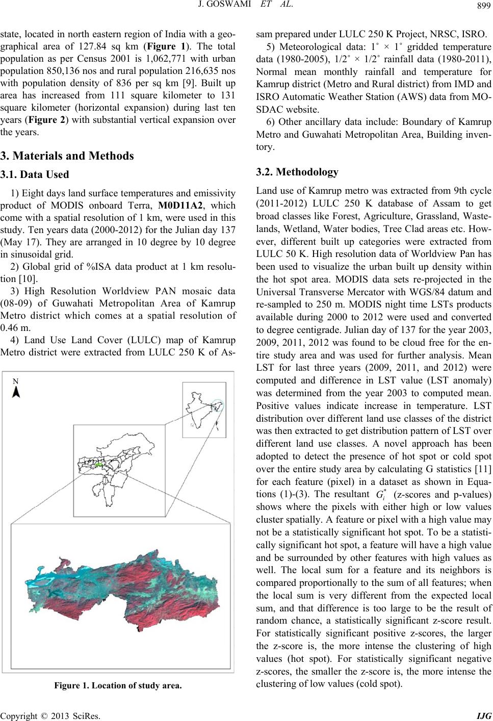
graphical area of 127.84 sq km (Figure 1). The total
population as per Census 2001 is 1,062,771 with urban
population 850,136 nos and rural population 216,635 nos
with population density of 836 per sq km [9]. Built up
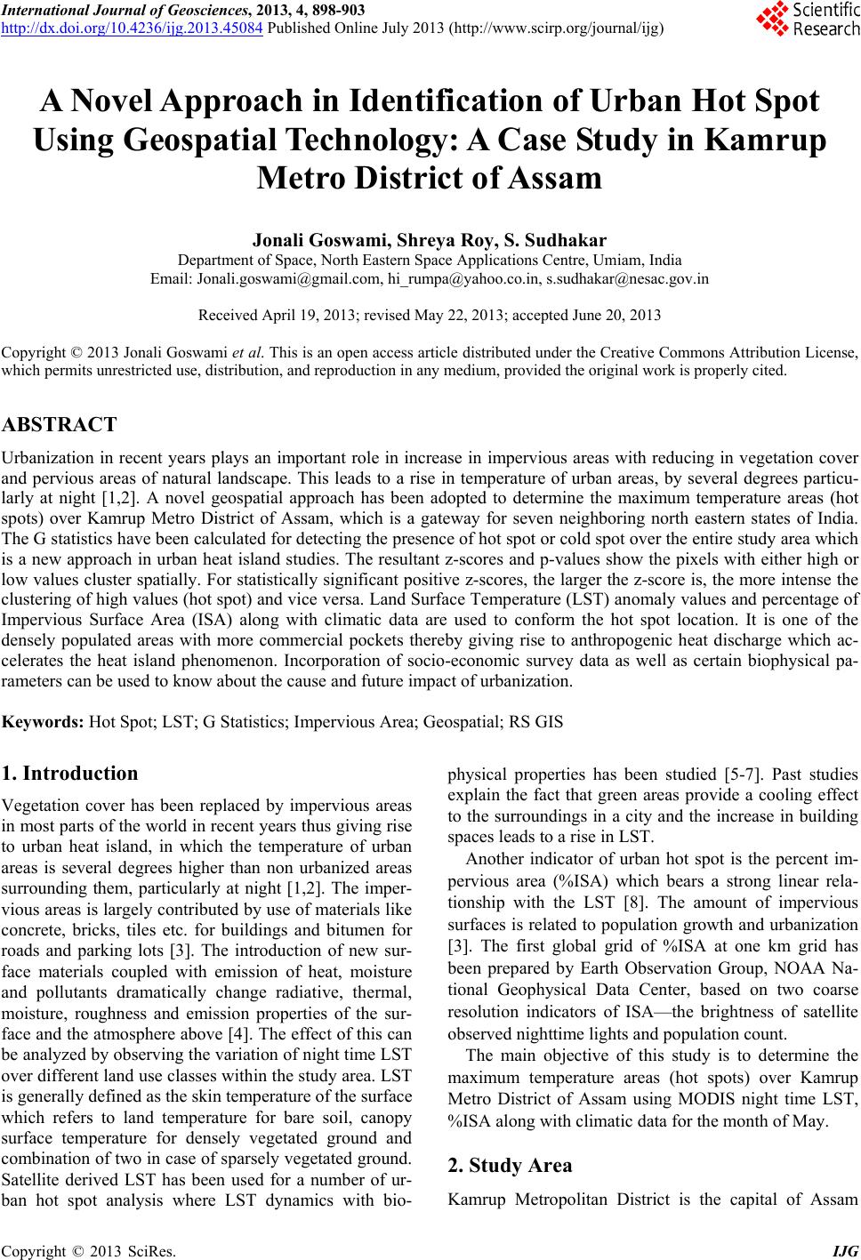
area has increased from 111 square kilometer to 131
square kilometer (horizontal expansion) during last ten
years (Figure 2) with substantial vertical expansion over
the years.
3. Materials and Methods
3.1. Data Used
1) Eight days land surface temperatures and emissivity
product of MODIS onboard Terra, M0D11A2, which
come with a spatial resolution of 1 km, were used in this
study. Ten years data (2000-2012) for the Julian day 137
(May 17). They are arranged in 10 degree by 10 degree
in sinusoidal grid.
2) Global grid of %ISA data product at 1 km resolu-
tion [10].
3) High Resolution Worldview PAN mosaic data
(08-09) of Guwahati Metropolitan Area of Kamrup
Metro district which comes at a spatial resolution of
0.46 m.
4) Land Use Land Cover (LULC) map of Kamrup
Metro district were extracted from LULC 250 K of As-
N
Figure 1. Location of study area.
sam prepared under LULC 250 K Project, NRSC, ISRO.
5) Meteorological data: 1˚ × 1˚ gridded temperature
data (1980-2005), 1/2˚ × 1/2˚ rainfall data (1980-2011),
Normal mean monthly rainfall and temperature for
Kamrup district (Metro and Rural district) from IMD and
ISRO Automatic Weather Station (AWS) data from MO-
SDAC website.
6) Other ancillary data include: Boundary of Kamrup
Metro and Guwahati Metropolitan Area, Building inven-
tory.
3.2. Methodology
Land use of Kamrup metro was extracted from 9th cycle
(2011-2012) LULC 250 K database of Assam to get
broad classes like Forest, Agriculture, Grassland, Waste-
lands, Wetland, Water bodies, Tree Clad areas etc. How-
ever, different built up categories were extracted from
LULC 50 K. High resolution data of Worldview Pan has
been used to visualize the urban built up density within
the hot spot area. MODIS data sets re-projected in the
Universal Transverse Mercator with WGS/84 datum and
re-sampled to 250 m. MODIS night time LSTs products
available during 2000 to 2012 were used and converted
to degree centigrade. Julian day of 137 for the year 2003,
2009, 2011, 2012 was found to be cloud free for the en-
tire study area and was used for further analysis. Mean
LST for last three years (2009, 2011, and 2012) were
computed and difference in LST value (LST anomaly)
was determined from the year 2003 to computed mean.
Positive values indicate increase in temperature. LST
distribution over different land use classes of the district
was then extracted to get distribution pattern of LST over
different land use classes. A novel approach has been
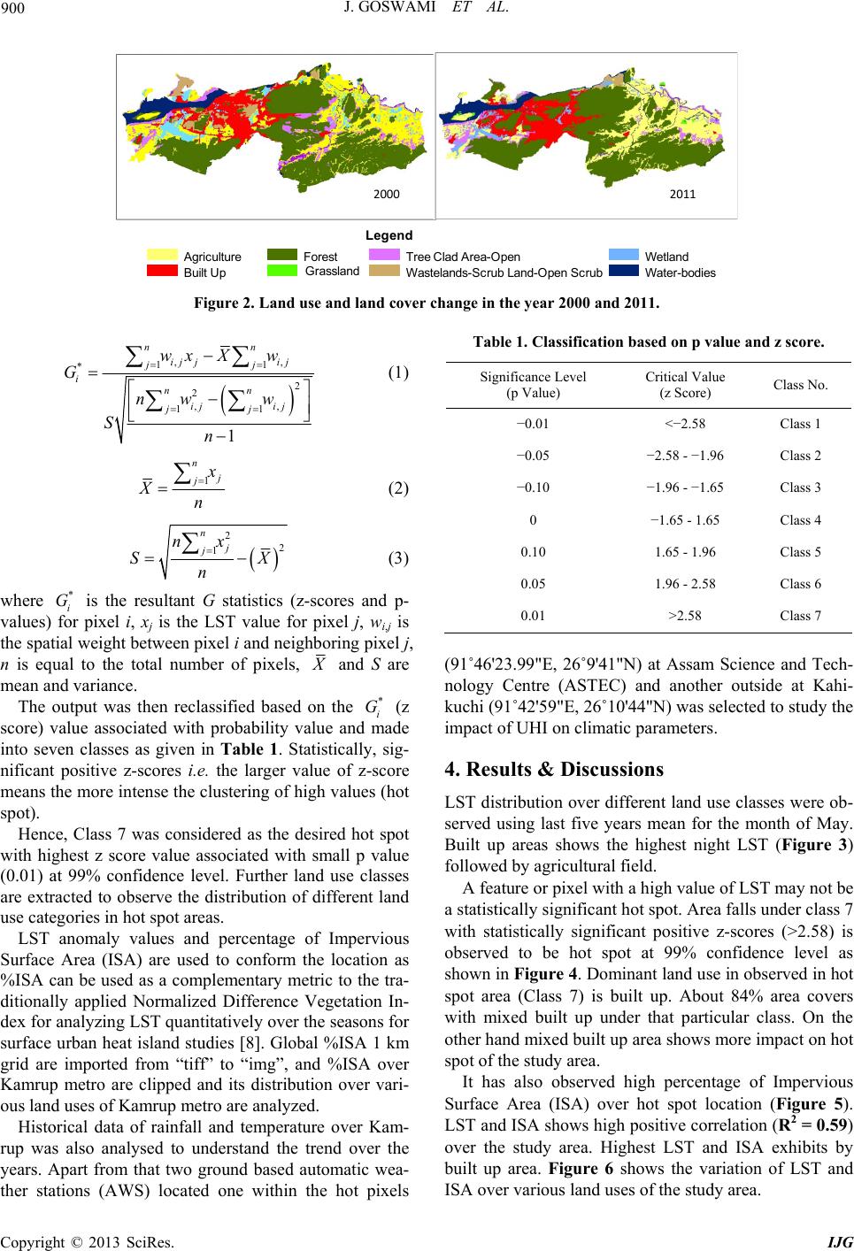
adopted to detect the presence of hot spot or cold spot
over the entire study area by calculating G statistics [11]
for each feature (pixel) in a dataset as shown in Equa-
tions (1)-(3). The resultant i (z-scores and p-values)
shows where the pixels with either high or low values
cluster spatially. A feature or pixel with a high value may
not be a statistically significant hot spot. To be a statisti-
cally significant hot spot, a feature will have a high value
and be surrounded by other features with high values as
well. The local sum for a feature and its neighbors is
compared proportionally to the sum of all features; when
the local sum is very different from the expected local
sum, and that difference is too large to be the result of
random chance, a statistically significant z-score result.
For statistically significant positive z-scores, the larger
the z-score is, the more intense the clustering of high
values (hot spot). For statistically significant negative
z-scores, the smaller the z-score is, the more intense the
lustering of low values (cold spot).
*
G
c
Copyright © 2013 SciRes. IJG
J. GOSWAMI ET AL.
Copyright © 2013 SciRes. IJG
900
Legend
Tree Clad Area-Open
Wastelands-Scrub Land-Open ScrubWetland
Water - bodi es
Forest
G rassland
Agriculture
Built Up
2000 2011
Figure 2. Land use and land cover change in the year 2000 and 2011.

1
*
2
ij j
i
ij
jwx
G
nw
Sn
,,
1
2
,,
11
1
nn
ij
j
nn
ij
jj
w
w
X






(1)
Table 1. Classification based on p value and z score.
Significance Level
(p Value)
Critical Value
(z Score) Class No.
0.01 <2.58 Class 1
0.05 2.58 - 1.96 Class 2
0.10 1.96 - 1.65 Class 3
0 1.65 - 1.65 Class 4
0.10 1.65 - 1.96 Class 5
0.05 1.96 - 2.58 Class 6
0.01 >2.58 Class 7
1
n
j
j
Xn
x
(2)

2
2
1
n
j
j
nxX
n
*
G
S (3)
where i is the resultant G statistics (z-scores and p-
values) for pixel i, xj is the LST value for pixel j, wi,j is
the spatial weight between pixel i and neighboring pixel j,
n is equal to the total number of pixels,
X
and S are
mean and variance.
(91˚46'23.99"E, 26˚9'41"N) at Assam Science and Tech-
nology Centre (ASTEC) and another outside at Kahi-
kuchi (91˚42'59"E, 26˚10'44"N) was selected to study the
impact of UHI on climatic parameters.
The output was then reclassified based on the i (z
score) value associated with probability value and made
into seven classes as given in Table 1. Statistically, sig-
nificant positive z-scores i.e. the larger value of z-score
means the more intense the clustering of high values (hot
spot).
*
G
4. Results & Discussio ns
LST distribution over different land use classes were ob-
served using last five years mean for the month of May.
Built up areas shows the highest night LST (Figure 3)
followed by agricultural field.
Hence, Class 7 was considered as the desired hot spot
with highest z score value associated with small p value
(0.01) at 99% confidence level. Further land use classes
are extracted to observe the distribution of different land
use categories in hot spot areas.
A feature or pixel with a high value of LST may not be
a statistically significant hot spot. Area falls under class 7
with statistically significant positive z-scores (>2.58) is
observed to be hot spot at 99% confidence level as
shown in Figure 4. Dominant land use in observed in hot
spot area (Class 7) is built up. About 84% area covers
with mixed built up under that particular class. On the
other hand mixed built up area shows more impact on hot
spot of the study area.
LST anomaly values and percentage of Impervious
Surface Area (ISA) are used to conform the location as
%ISA can be used as a complementary metric to the tra-
ditionally applied Normalized Difference Vegetation In-
dex for analyzing LST quantitatively over the seasons for
surface urban heat island studies [8]. Global %ISA 1 km
grid are imported from “tiff” to “img”, and %ISA over
Kamrup metro are clipped and its distribution over vari-
ous land uses of Kamrup metro are analyzed.
It has also observed high percentage of Impervious
Surface Area (ISA) over hot spot location (Figure 5).
LST and ISA shows high positive correlation (R2 = 0.59)
over the study area. Highest LST and ISA exhibits by
built up area. Figure 6 shows the variation of LST and
ISA over various land uses of the study area.
Historical data of rainfall and temperature over Kam-
rup was also analysed to understand the trend over the
years. Apart from that two ground based automatic wea-
ther stations (AWS) located one within the hot pixels
J. GOSWAMI ET AL. 901
21.6
21.8
22.0
22.2
22.4
22.6
22.8
23.0
Nighttime LST(°C)
Landuseclass
Figure 3. Distribution of LST over different land use
classes.
8.2% 0.7%
0.7
84.2%
4.7%
1.4%
%
Forest
waterbodies
Wetland
BuiltUpBuiltUp(Urban)Recreational
BuiltUpBuiltUp(Urban)Transportati on
BuiltUpBuiltUp(Urban)MixedBuiltUparea
Figure 4. Spatial location of hot spot and land covers dis-
tribution (percent area) in hot spot area.
Figure 5. Spatial view of percentage ISA.
LST anomaly has been worked out using cloud free
data of same period of the year 2003. Highest anomaly is
also observed in and around hot spot areas (Figure 7).
Maximum anomaly observed mainly in built up area fol-
lowed by tree clad area, which mostly includes small
huts with homestead garden and agricultural field par-
ticularly current fallow land.
While the surface urban hot spot is typically charac-
terized as land surface temperature (LST), atmospheric
urban hot spot are normally measured by in situ sensors
of air temperature via weather station networks [8]. It has
been observed (Figure 8) that over the last decade there
is an increasing trend in maximum temperature from
May to October over Kamrup (Metro and Rural district)
as compared to normal from 1971-2000. Similarly there
is a decreasing trend in rainfall pattern as compared to
last two decades particularly from May-September. Pre
and post monsoon has also shown decreasing trend as
shown in Figure 9. Pre monsoon and post monsoon also
shows an inverse relation over the years.
Similarly analysis has been done to see the tempera-
ture and rainfall variation over Kamrup district particu-
larly in the month of May (Figure 10). It has been ob-
served that there is an increasing trend of maximum tem-
perature with decrease in rainfall activity from 1995 on-
wards. Figure 11 also shows that there is an increase in
21.6
21.8
22
22.2
22.4
22.6
22.8
23
0.0
2.0
4.0
6.0
8.0
10.0
12.0
14.0
16.0
18.0 ISA
LST
ISA(%)
NightLST(°C)
Figure 6. Variation of LST and ISA over various land use
classes.
Figure 7. LST anomaly for a period of 10 years. (Positive
anomaly indi cates increas e in temperature.)
Copyright © 2013 SciRes. IJG
J. GOSWAMI ET AL.
902
22
24
26
28
30
32
Temp(°C)
Month
200010
Normal
0
10
20
30
40
1 3 5 7 91113151719212325272931
Temperature(°C)
Days
0
100
200
300
400
Rainfall(mm)
Month
198090
199000
200010
Figure 8. Monthly decadal temperature and rainfall distri-
bution over Kamrup.
120
100
80
60
40
20
0
20
40
60
2004 2005 2006 2007 2008 2009
%RainfallDeparture
2010 2011
PreMonsoon Monsoon PostMonsoon
Figure 9. Pre, post and monsoonal rainfall departure over
Kamrup for last eight years
27.0
28.0
29.0
30.0
31.0
32.0
0
100
200
300
400
Rainfall(m m)
Years
Rainfall Temper a ture
Temperature(°C)
Figure 10. Rainfall and temperature variation for the
month of May over Kamrup.
maximum temperature with decrease in rainfall activity
within the hot pixel area.
In the study district, hot spot have been identified in
the areas of the densely populated area with more com-
mercial pockets thereby giving rise to anthropogenic heat
discharge which accelerates the heat island phenomenon.
The location of the urban hot spot shows both rise in
0
10
20
30
40
50
60
1 3 5 7 911131517202224262830
Rainf all(mm)
Days
Figure 11. Temperature and rainfall variation over hot
pixel area (ASTEC) and outside the hot pixel area (Kahi-
kuchi) for the month of May, 2012.
surface and atmospheric temperature.
5. Conclusion
This study investigates the use of G statistics in deter-
mining the unusual pattern of spatial association which is
significantly different to what is generally observed
across the whole study area. Results indicate %ISA is an
important indicator of rise in surface temperature with
positive linear relationship between LST. Vegetation co-
ver provides a cooling effect to the surroundings. Thus,
in the future city planning and development more atten-
tion should be paid to urban greening and a minimum
available space between the buildings. A new concept of
urban farming is also in the picture now a day. However,
the shortcoming in this case study is unavailability of
cloud free satellite data for other seasons as well. There
is also a lack of a good network of ground based obser-
vation on climatic parameters. This study can be at-
tempted with high resolution satellite data and other so-
cio-economic survey data to know about the cause and
future impact of urban heat island.
REFERENCES
[1] D. R. Streutker, “A Remote Sensing Study of the Urban
Heat Island of Houston, Texas,” International Journal of
Remote Sensing, Vol. 23, No. 13, 2002, pp. 2595-2608.
doi:10.1080/01431160110115023
[2] J. A. Voogt and T. R. Oke, “Thermal Remote Sensing of
Urban Climates,” Remote Sensing of Environment, Vol.
86, No. 3, 2003, pp. 370-384.
Copyright © 2013 SciRes. IJG
J. GOSWAMI ET AL.
Copyright © 2013 SciRes. IJG
903
doi:10.1016/S0034-4257(03)00079-8
[3] S. J. Stanwoski, “Population Density as an Indirect Indi-
cator of Urban and Sub-Urban Land Surface Modifica-
tions,” US Geological Survey, pp. B219-B224.
[4] M. Roth, “Effects of Cities on Local Climates,” Proceed-
ings of Workshop of Institute for Global Environment
Studies/Asia-Pacific Network (IGES/APN), Kitakyushu,
23-25 January, p. 13.
[5] B. R. Parida, B. Oinam, N. R. Patel, N. Sharma, R. Kand-
wal and M. K. Hazarika, “Land Surface Temperature Va-
Riation in Relation to Vegetation Type Using MODIS
Satellite Data in Gujarat State of India,” International
Journal of Remote Sensing, Vol. 29, No. 14, 2008, pp.
4219-4235. doi:10.1080/01431160701871096
[6] S. Dumitrescu and S. Cheval, “The July Urban Heat Is-
land of Bucharest as Derived from MODIS Images,”
Theoretical and Applied Climatology, Vol. 96, No. 1-2,
2009, pp. 145-153.
[7] S. Khandelwal, R. Goyal, N. Kaul and V. Singhal, “Study
of Land Surface Temperature Variations with Distance
from Hot Spots for Urban Heat Island Analysis,” Geospa-
tial World Forum, Theme Dimensions and Directions of
Geospatial Industry, 18-21 January 2011, Hyderabad.
[8] F. Yuan and M. E. Baur, “Comparison of Impervious Sur-
face Area and Normalized Difference Vegetation Index as
Indicators of Surface Urban Heat Island Effects in Land-
sat Imagery,” Remote Sensing of Environment, Vol. 106,
No. 3, 2007, pp. 375-386. doi:10.1016/j.rse.2006.09.003
[9] District at a Glance. http://kamrupmetro.nic.in/glance.asp
[10] Global Distribution and Density of Constructed Impervi-
ous Surfaces.
http://ngdc.noaa.gov/eog/dmsp/download_global_isa.html
[11] A. Getis and J. K. Ord, “The Analysis of Spatial Associa-
tion by Use of Distance Statistics,” Geographical Analy-
sis, Vol. 24, No. 3, 1992, pp. 189-207.
doi:10.1111/j.1538-4632.1992.tb00261.x