Engineering, 2013, 5, 601-610
http://dx.doi.org/10.4236/eng.2013.57072 Published Online July 2013 (http://www.scirp.org/journal/eng)
Multi-Objective Optimization Using Genetic Algorithms
of Multi-Pass Turning Process
Abdelouahhab Jabri, Abdellah El Barkany, Ahmed El Khalfi
Faculty of Sciences and Technology, Department of Mechanical Engineering,
Sidi Mohammed Ben Abdellah University, Fez, Morocco
Received April 22, 2013; revised May 22, 2013; accepted June 1, 2013
Copyright © 2013 Abdelouahhab Jabri et al. This is an open access article distributed under the Creative Commons Attribution Li-
cense, which permits unrestricted use, distribution, and reproduction in any medium, provided the original work is properly cited.
ABSTRACT
In this paper we present a multi-optimization technique based on genetic algorithms to search optimal cuttings parame-
ters such as cutting depth, feed rate and cutting speed of multi-pass turning processes. Tow objective functions are si-
multaneously optimized under a set of practical of machining constraints, the first objective function is cutting cost and
the second one is the used tool life time. The proposed model deals multi-pass turning processes where the cutting op-
erations are divided into multi-pass rough machining and finish machining. Results obtained from Genetic Algorithms
method are presented in Pareto frontier graphic; this technique helps us in decision making process. An example is pre-
sented to illustrate the procedure of this technique.
Keywords: Genetic Algorithms; Mutli-Objective Optimization; Turning Process; Machining
1. Introduction
Cutting parameters such as depth of cut, cutting speed
and feed rate influence directly on machining time and
cost, in addition these parameters have a great impact on
product quality. The objective of process planning is to
select appropriate cutting parameters which generate
maximum profit rate to the company and reach costumer
requirements in terms of product quality and lead time.
Cutting parameters are: cutting speed (V), feed rate (f)
and cutting depth (d), Figure 1 illustrates these parame-
ters. In the present paper we present a multi-objective
optimization technique of multi-pass turning processes
based on Genetic Algorithms. Indeed, tow objective
functions are simultaneously optimized which are the
cutting cost and the used tool life of cutting tool, subject
to a set of practical constraints like cutting force, ma-
chine power and surface quality.
Several previous research have dealt with cutting con-
ditions optimization by means of different techniques,
fuzzy logics, neural networks, simulated annealing, ge-
netic algorithms, colony optimization and practical swarm
optimization, etc.
Tsai [1] studied the relationship between the multi-
pass machining and single-pass machining. He presented
the concept of a break-even point, i.e. there is always a
point, a certain value of depth of cut, at which sin-
gle-pass and double-pass machining are equally effective.
When the depth of cut drops below the break-even point,
the single-pass is more economical than the double-pass,
and when the depth of cut rises above this break-even
point, double-pass is better. Carbide tools are used to turn
the carbon steel work material.
Chua [2] used a sequential quadratic programming
technique for optimizing the cutting conditions for multi-
pass turning operations. Shin and Joo [3] proposed a
mathematical model for the multi-pass turning process,
which was subsequently used by many researchers.
Figure 1. Cutting parameters of a turning operation.
C
opyright © 2013 SciRes. ENG

A. JABRI ET AL. 602
Agapiou [4] formulated single-pass and multi-pass ma-
chining operations. Production cost and total time were
taken as objectives and a weighting factor was assigned
to prioritize, the two objectives in the objective function.
He optimized the number of passes, depth of cut, cutting
speed and feed rate in his model, through a multi-stage
solution process called dynamic programming. Several
physical constraints were considered and applied in his
model. In his solution methodology, every cutting pass is
independent of the previous pass; hence the optimality
for each pass is not reached simultaneously.
A feed-forward neural network was used by Wang [5]
for solving the multi-objective problem, which involved
productivity, operation cost and cutting quality. Gupta [6]
worked on the optimality of depth of cut of the multi-
pass turning operation using an integer programming
model. Chen and Tsai [7] applied the simulated anneal-
ing approach to solve the optimization problem for
minimum unit production costs of the multi-pass turning
process. Kee [8] outlined the optimization strategies for
multi-pass rough turning on conventional and CNC
lathes with practical constraints, such as force and power.
Nian [9] carried out the optimization of turning opera-
tions based on the Taguchi method and considered vari-
ous multiple performance characteristics, such as tool life,
cutting force, and surface finish. Alberti and Perrone [10]
used the genetic algorithm to solve a fuzzy probabilistic
optimization model for determining the cutting parame-
ters.
Arezoo [11] developed an expert system to select cut-
ting tools and conditions of turning operations using
Prolog. The system can select the tool holder, and the
insert and cutting conditions, such as cutting speed, feed
rate and depth of cut. Dynamic programming was used to
optimize the cutting conditions. Dereli [12] developed an
optimization system for cutting parameters of prismatic
parts based on genetic algorithms. Onwubolu and Ku-
malo [13] used the mathematical model of Chen and Tsai
[7] and applied the genetic algorithm to minimize the
unit production cost. Al-Ahmari [14] presented a nonlin-
ear programming model for the optimization of machin-
ing parameters and subdivisions of the depth of cut in
multi-pass turning operations. Wang [15] used the ge-
netic algorithm to select optimal cutting parameters and
cutting tools in multi-pass turning operations with more
focus on the tool wear and chip breakability aspects of
the process.
Vijayakumar [16] used the ant colony optimization
algorithm and attempted the same mathematical model as
Chen and Tsai [7] and Onwubolu and Kumalo [13].
Franci and Joze [17] proposed a multi-objective optimi-
zation technique based on Genetic Algorithm where cut-
ting cost, cutting time and surface quality are optimized
simultaneously. Zuperl [18] proposed a hybrid optimiza-
tion technique for complex optimization of cutting pa-
rameters; this optimization technique is based on the Ar-
tificial Neural Network ANN and OPTIS routine.
Wang and Jawahir [19] proposed a new GA-based
methodology, whose research was focused on the selec-
tion of different cutting tools for different passes of turn-
ing operations and allocation of the depth of cut. Sardi-
nas [20] used the micro-genetic algorithm for attempting
the multi-objective optimization model and obtained the
Pareto front result. Cus and Zuperl [21] proposed an op-
timization technique based on Artificial Neural Network
to solve the same problem studied by Franci and Joze
[17].
Abburi and Dixit [22] developed an optimization meth-
odology, which was a combination of a real coded ge-
netic algorithm and sequential quadratic programming, to
obtain Pareto optimal solutions for minimizing the pro-
duction cost. Yildiz [23] attempted the same mathe-
matical model as Vijayakumar [16] using the hybrid Ta-
guchi harmony search algorithm. Ojha [24] used a neural
network fuzzy set and genetic algorithm-based soft
computing methodology to optimize process parameters
in multi-pass turning operations. Srinivas [25] used par-
ticle swarm intelligence for selecting the optimum ma-
chining parameters in multi-pass turning operations.
Deepak [26] used a geometric programming method to
optimize the production time of turning process; in this
technique, only cutting speed and feed rate are taken in
consideration. venkata and kaliyankar [27] the parameter
optimization of a multi-pass turning operation was car-
ried out using an optimization algorithm, named, the
teaching-learning-based optimization algorithm. For de-
tailed literature review, see Aggarwal [28] and Deepak
[29].
The above mentioned efforts show the interest of se-
lecting optimal cutting parameters in turning process.
Almost all research papers have dealt with multi-pass
process turning; in our study we propose an optimization
of multi-pass turning process where two objective func-
tions are optimized simultaneously: cutting cost and used
tool life of cutting tool.
2. Multi Pass Turning Process Model
The goal of this multi-optimization cutting model is to
determine the optimal machining parameters “cutting
speed, feed rate, and cutting depth” in order to minimize
simultaneously the cutting cost and the used tool life of a
multi pass turning process; In other words this turning
process has multiple rough cut and a single finish cut.
Therefore, this optimization model includes six machin-
ing parameters (Vr, fr, dr, Vf, ff, df): the three first pa-
rameters for rough machining and the last three parame-
ters are for finishing operation.

A. JABRI ET AL. 603
2.1. Notation Used in the Cutting Model
m
C cutting cost by actual time in cut ($/piece),
o
K
direct labor cost + overhead ($/min),
D, L diameter and length of work-piece (mm),
n number of rough cuts as integer
T, Tr, Tf tool life, expected tool life for rough machining,
and expected tool life, for finish machining (min),
Tp tool life of weighted combination of Tf and Tr (min),

a weight for Tp [0, 1],
TU, TL upper and lower bounds for tool life (min),
t
d depth of material to be removed (mm),
0,,,C pqr constants of the tool-life equation,
1,,K

 constants of cutting force equation,
2,,,K

 constants related to equation of chip-tool
interface temperature,
R Surface roughness
a
R
nose radius of cutting tool (mm),
U
SR maximum allowable surface roughness (mm),
U
F
maximum allowable cutting force (kgf),
U
P maximum allowable cutting power (kW),
power efficiency,
,
rf
QQ chip-tool interface rough and finish machining
temperatures(˚C),
U
Q maximum allowable chip-tool interface
temperature (˚C),
,
rL rU
VV lower and upper bound of cutting speed in
rough machining (m/min),
,
rL rU
dd lower and upper bound of depth of cut in
rough machining (mm),
,
rL rU
f
f lower and upper bound of feed rate in rough
machining (mm/rev),
,
f
LfU
VV lower and upper bound of cutting speed in
finish machining (m/min),
,
f
LfU
dd lower and upper bound of depth of cut in
finish machining (mm),
,
f
LfU
f
f Lower and upper boud of feed rate in finish
machining (mm/rev),
2.2. Objective Functions
In this model, we adopt the same components considered
in the previous works related to multi-pass turning proc-
ess: [3,7,13].
2.2.1. Cutti ng Cost
According to [3], the unit production cost for the multi
pass turning operations problem consists of four basic
cost components:
 Cutting cost by actual time in cutting operation,
 Machine idle cost due to loading and unloading op-
erations and idle tool motion,
 Cost for tool replacement,
 Tool cost.
In this work, we consider only the Cutting cost for
multi-pass turning process, it is expressed as:
mo
CKt
m

 (1)
where: tm is the cutting time of the actual operation [3].
Since the operation is a multi-pass, tm can be divided
into two parts; therefore it is expressed as the sum of
roughing and finishing operations times:
mmrmf
tt t

 (2)
where:
1000 1000
tf
mr
rrrr r
dd
DL DL
tn
VfVf d







(3)
1000
mf
f
f
DL
tVf

 (4)
Finally, based on the above equations, the cutting cost
can be expressed as:
1000 1000
tf
mo
rrrf f
dd
DL DL
CK VfdV f


 

 




 


(5)
2.2.2. Used Tool Life
The second objective function is the used tool life ξ, it is
considered as the part of the whole tool life which is
consumed in the process:

100%
1
mf
mr
rf
t
t
TT









(6)
where: Tr and Tf are the Taylor tool life of roughing and
finishing operations, respectively [30].

1000
1000 100%
1
tf
ff
rr r
rf
dd DL
DL
Vf
Vf d
TT



 











(7)
0
r
p
qr
rrr
C
TVfd  (8)
0
fpqr
f
ff
C
TVfd  (9)
2.3. Machining Constraints
Several constraints are taken in consideration in this
model; some of these limitations are the allowed values
of cutting parameters (cutting speed V, feed rate f and
cutting depth d), given by the tool maker, and limited by

A. JABRI ET AL. 604
the bottom and top permissible limits.
For the selected tool the tool maker specifies the limi-
tations of the cutting conditions. The limitation on the
machine is the cutting power and the cutting force. Simi-
larly, the machining characteristics of the work piece
material are determined by physical properties. The con-
sumption of the power [3] can be expressed as the func-
tion of the cutting force and cutting speed:
6120
F
V
P

 (10)
where η is the mechanical efficiency of the machine and
F is given by the following formula [3]:
1
F
Kf d


 (11)
Other limitations that will be taken into account are:
surface finish constraint [31] and chip-tool interface tem-
perature constraint, [32].
2
QKVfd


 (12)
2
8a
f
RR  (13)
2.4. Final Cutting Model
Based on the previous equations, the optimization model
for multi pass turning operation can be formulated as
shown below:
min 1000 1000
tf
mo
rrrff
dd
DL DL
CK VfdV f


 



















(14)

1000
1000
min 100%
1
tf
ff rr r
rf
dd DL
DL
Vf
Vf d
TT


 






 
















(15)
Subject to:
Roughing:
rL rrU
VVV (16)
rL r rU
ddd (17)
rL rrU
f
ff (18)
rU
F
F (19)
rU
PP (20)
r
QQU (21)
Finishing:
f
Lf fU
VVV (22)
f
Lff
ddd
f
Lf fU
f
ff

 (24)
f
U
FF (24)
f
U
PP (26)
f
U
QQ (27)
f
U
RSR (28)
The cutting model formulated above is non-linear con-
strained programming (NCP) problem with multiple con-
tinuous variables referred to as the machining parameters.
The machining parameters in roughing and finishing are
dependent intrinsically, hence they are analyzed simul-
taneously. The proposed genetic algorithm optimization
technique that is capable of solving the complex problem
is described below.
3. Optimization Algorithm
3.1. Genetic Algorithms
Genetic Algorithms (GA) are search algorithms based on
the mechanics of natural selection and natural genetics
[33]. GA then iteratively creates new populations from
the old by ranking the strings and interbreeding the fittest
to create new, and conceivably better, populations of
strings which are (hopefully) closer to the optimum solu-
tion to the problem at hand. So in each generation, the
GA creates a set of strings from the bits and pieces of the
previous strings, occasionally adding random new data to
keep the population from stagnating. The end result is a
search strategy that is tailored for vast, complex, multi-
modal search spaces. GA is a form of randomized search,
in that the way in which strings are chosen and combined
is a stochastic process; Figure 2 shows a flow chart of
EvaluateS(t)
Select S(t) from
S(t-1)
Diversify S(t)
IntensifyS(t)
EvaluateS(t)
End
Stopping condition
Initialize solution
space S(0)
U
(23) Figure 2. Flowchart of the basic genetic algorithm steps, [13].

A. JABRI ET AL. 605
geneticalgorithm method, [13].
3.2. Basic Genetic Algorithm Operations
There are three basic operators found in every genetic
algorithm: initialization, evaluation, selection, diversifi-
cation and intensification.
3.2.1. Initialization
The first step of GA is the generation of the individuals
for the initial population. Randomly generated strings of
Feed rate, speed and depth of cut form the solution space
(popsize). These strings are generated between the limits:
 Feed rate: [frL, frU] and [ffL, ffU] for the roughing and
finishing conditions respectively.
 Speed: [VrL, VrU] and [VfL, VfU] for the roughing and
finishing conditions respectively.
 Depth of cut: [drL, drU] and [dfL, dfU] for the roughing
and finishing conditions respectively.
3.2.2. Evaluation
This operation allows individual strings to be copied for
possible inclusion in the next generation. The chance that
a string will be copied is based on the string’s fitness
value, calculated from a fitness function. For each gen-
eration, the reproduction operator chooses strings that are
placed into a mating pool, which is used as the basis for
creating the next generation.
A score (objective) function is calculated, it represents
the score for each strings of the solution space and the
string that has the maximum score function value is de-
termined. For an optimization problem where there is a
function to be minimized, the competitiveness of the ith
solution


i
f
t is obtained as follows:
 
max
iii
f
tf gt (29)
where

i
g
t is the objective function of a string and
fmax is the least objective function value in the current
solution space. The corresponding selection probability
P(i) is equal to:




popsize
1
i
i
k
ft
Pi
f
t

 (30)
The most competitive solution strings are affected by a
higher probability of sampling, for advancement to sub-
sequent state.
There are six alternate selection schemes presented in
[33] deterministic sampling, remainder stochastic sam-
pling without replacement, remainder stochastic sam-
pling with replacement, stochastic sampling without re-
placement, stochastic sampling with replacement, and
stochastic tournament. The remainder stochastic sam-
pling without replacement is superior to other five strate-
gies [33] and is the one used in the work reported here. In
this strategy, the expected count ei is calculated as usual:



popsize
1
p
opsize
i
ii
k
ft
eft

 (31)
The fractional parts of ei are treated as probabilities.
One by one, weighted coin tosses are performed using
the fractional parts as success probabilities. The strings
receive copies equal to the whole parts of ei.
3.2.3. Cross ov er Operation
Crossover in biological terms refers to the blending of
chromosomes from the parents to produce new chromo-
somes for the offspring. The analogy carries over to
crossover in Gas. The GA selects two strings at random
from the mating pool and then calculates whether cross-
over should take place using a parameter called the
crossover probability (pcross). If the GA decides not to
perform crossover, the two selected strings are simply
copied to the new population. If crossover does take
place, then a random splicing point is chosen in a string,
the two strings are spliced and the spliced regions are
mixed to create two (potentially) new strings. These child
strings are then placed in the new population. As an ex-
ample, we present a two-point crossover on a binary
number. The following strings are selected for crossover:
String 1: 000000000000001^001^110.
String 2: 000000000000001^101^100.
where: “^” represents the cross positions.
After crossover operation, the newly created strings
are:
New String 1: 000000000000001^101^110.
New String 2: 000000000000001^001^100.
3.2.4. Mut ation
Mutation is a random modification of a randomly se-
lected string. It guarantees the possibility of exploring the
space of solutions for any initial solution space so as to
permit a zone of local minimum to be abandoned. Muta-
tion is done with a mutation probability (Pmutate). Two
random integers r1, and r2 are selected from strings 1 and
2 respectively such that 1 1r

; 2 (block-size) and
12
rn
rr

. The GA procedure then inverts (from 0 to 1, or 1
to 0) string bits designated by positions r1 and r2. For
example, if r1 = 17 and r2 = 18, then the previous new
strings 1 and 2 (mutated positions are underlined) be-
come:
New String 1: 000000000000001001110.
New String 2: 000000000000001011100.
4. An Application Example
In this section an example is presented to illustrate the
proposed multi-objective optimization. As presented in
previous section two objective functions are optimized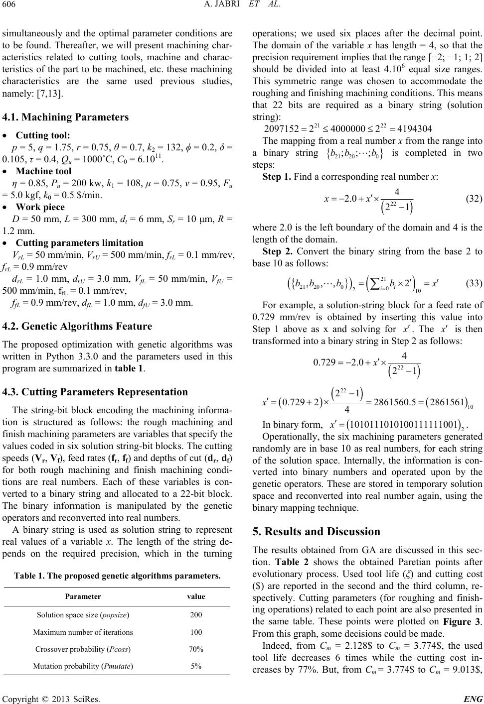

A. JABRI ET AL. 606
simultaneously and the optimal parameter conditions are
to be found. Thereafter, we will present machining char-
acteristics related to cutting tools, machine and charac-
teristics of the part to be machined, etc. these machining
characteristics are the same used previous studies,
namely: [7,13].
4.1. Machining Parameters
 Cutting tool:
p = 5, q = 1.75, r = 0.75, θ = 0.7, k2 = 132, ϕ = 0.2, δ =
0.105, τ = 0.4, Qu = 1000˚C, C0 = 6.1011.
 Machine tool
η = 0.85, Pu = 200 kw, k1 = 108, μ = 0.75, ν = 0.95, Fu
= 5.0 kgf, k0 = 0.5 $/min.
 Work piece
D = 50 mm, L = 300 mm, dt = 6 mm, Sr = 10 μm, R =
1.2 mm.
 Cutting parameters limitation
VrL = 50 mm/min, VrU = 500 mm/min, frL = 0.1 mm/rev,
frL = 0.9 mm/rev
drL = 1.0 mm, drU = 3.0 mm, VfL = 50 mm/min, VfU =
500 mm/min, ffL = 0.1 mm/rev,
ffL = 0.9 mm/rev, dfL = 1.0 mm, dfU = 3.0 mm.
4.2. Genetic Algorithms Feature
The proposed optimization with genetic algorithms was
written in Python 3.3.0 and the parameters used in this
program are summarized in table 1.
4.3. Cutting Parameters Representation
The string-bit block encoding the machining informa-
tion is structured as follows: the rough machining and
finish machining parameters are variables that specify the
values coded in six solution string-bit blocks. The cutting
speeds (Vr, Vf), feed rates (fr, ff) and depths of cut (dr, df)
for both rough machining and finish machining condi-
tions are real numbers. Each of these variables is con-
verted to a binary string and allocated to a 22-bit block.
The binary information is manipulated by the genetic
operators and reconverted into real numbers.
A binary string is used as solution string to represent
real values of a variable x. The length of the string de-
pends on the required precision, which in the turning
Table 1. The proposed genetic algorithms parameters.
Parameter value
Solution space size (popsize) 200
Maximum number of iterations 100
Crossover probability (Pcoss) 70%
Mutation probability (Pmutate) 5%
operations; we used six places after the decimal point.
The domain of the variable x has length = 4, so that the
precision requirement implies that the range [−2; −1; 1; 2]
should be divided into at least 4.106 equal size ranges.
This symmetric range was chosen to accommodate the
roughing and finishing machining conditions. This means
that 22 bits are required as a binary string (solution
string):
21 22
209715224000000 24194304 
The mapping from a real number x from the range into
a binary string


21 200
;;;bb b is completed in two
steps:
Step 1. Find a corresponding real number x:

22
4
2.0 21 xx

  (32)
where 2.0 is the left boundary of the domain and 4 is the
length of the domain.
Step 2. Convert the binary string from the base 2 to
base 10 as follows:




21
21 2000
210
,,, 2
i
i
bb bbx




 (33)
For example, a solution-string block for a feed rate of
0.729 mm/rev is obtained by inserting this value into
Step 1 above as x and solving for
x
. The
x

is then
transformed into a binary string in Step 2 as follows:

22
4
0.729 2.021 x  




22
10
21
0.729 22861560.52861561
4
x
 
In binary form,


2
Operationally, the six machining parameters generated
randomly are in base 10 as real numbers, for each string
of the solution space. Internally, the information is con-
verted into binary numbers and operated upon by the
genetic operators. These are stored in temporary solution
space and reconverted into real number again, using the
binary mapping technique.
10101110101 0011 111100 1x.
5. Results and Discussion
The results obtained from GA are discussed in this sec-
tion. Table 2 shows the obtained Paretian points after
evolutionary process. Used tool life (ξ) and cutting cost
($) are reported in the second and the third column, re-
spectively. Cutting parameters (for roughing and finish-
ing operations) related to each point are also presented in
the same table. These points were plotted on Figure 3.
From this graph, some decisions could be made.
Indeed, from Cm = 2.128$ to Cm = 3.774$, the used
tool life decreases 6 times while the cutting cost in-
creases by 77%. But, from C = 3.774$ to Cm = 9.013$,
m

A. JABRI ET AL. 607
Table 2. Pareto front points generated by the proposed optimization technique.
N˚ Cm ($) ζ (%) fr (mm/rev) dr (mm) Vr (m/min) ff (mm/rev) df (mm) Vf (m/min)
1 2.128 27.780 0.258 1.231 212.127 0.193 1.303 250.777
2 2.251 22.064 0.258 1.231 212.128 0.193 1.428 186.777
3 2.546 13.081 0.116 2.289 208.381 0.240 1.309 177.725
4 2.951 8.887 0.115 2.287 176.138 0.241 1.309 173.600
5 3.303 6.758 0.163 1.749 157.624 0.297 1.030 113.811
6 3.619 5.006 0.106 2.468 165.480 0.139 1.962 119.811
7 3.774 3.963 0.115 2.373 144.219 0.166 1.634 121.162
8 5.003 1.684 0.142 1.994 101.711 0.120 2.197 103.352
9 5.543 1.214 0.114 2.376 94.075 0.131 2.056 94.648
10 6.242 0.899 0.133 2.135 82.057 0.118 2.106 86.302
11 7.044 0.530 0.103 2.628 75.415 0.231 1.371 60.907
12 8.056 0.435 0.207 1.486 60.565 0.177 1.566 54.171
13 9.013 0.274 0.127 2.205 55.618 0.226 1.332 52.609
Used tool life ζ (%)
Cutting cost ($)
2 3 4 5 6 7 8 9 10
30
25
20
15
10
5
0
Figure 3. Pareto Front.
the used tool life decreases drastically, however the cut-
ting cost increases by 140%. For a normal state, it is clear
that the point (Cm = 3.774$ and ξ = 4%) is to be selected
point 7 in Table 2.
After this point: cutting cost increases but the other
hand we do not gain great reduction of used tool life;
before this value (3.774$ and ξ = 4%), cutting cost is
reduced but used tool life is more and more greater
which could increases strongly the total cutting cost.
In terms of cost, the cost selected tool edge is 14.17$,
which means that the tool cost of this operation is 0.5$
and cutting cost is 4$. After this point cutting tool cost is
reduced to 0.25$ but which means that we gain 0.25$ but
in the other hand cutting cost increase by 1$, Figure 4.
The total cost of cutting operation is the sum of cutting
cost and the tool cost. Figure 4 presents the sum of these
two entities of each points of Table 2. From this graph it
is clear that: points from 4 to 7 are optimal values of cut-
ting cost and used cutting tool.
Figure 5 presents objective functions (Used tool life
and cutting cost) in function of feed rate and cutting
speed. From these figures it is clear that:
 Used tool life increases with cutting speed,
 Cutting cost decreases with cutting speed.
Minimum cutting cost is achieved for maximal values
of cutting speed, however for minimal used tool life, lit-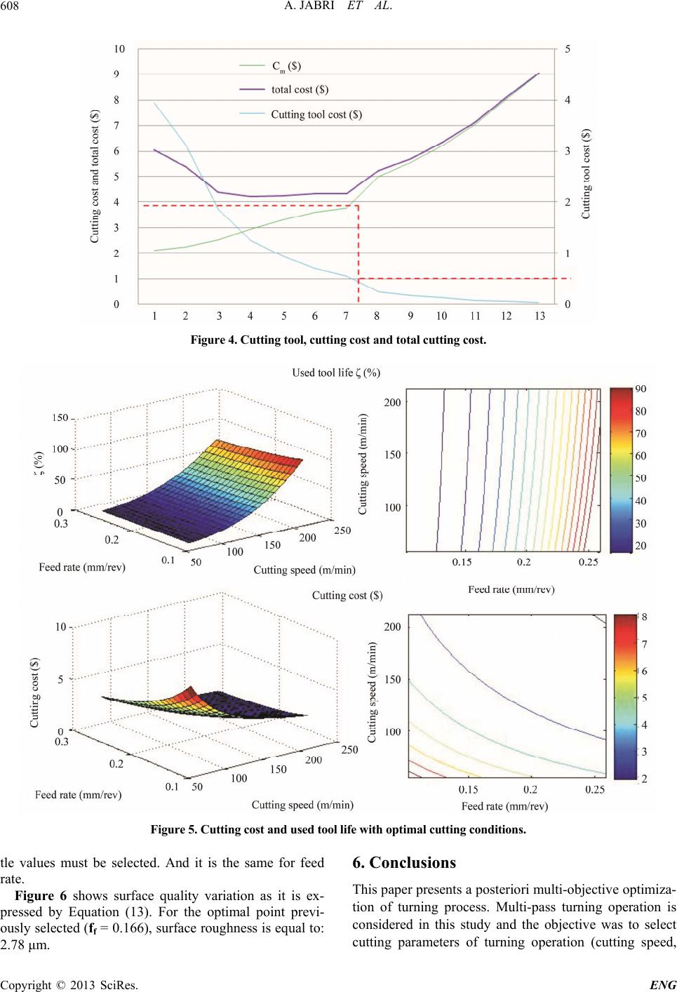

A. JABRI ET AL. 608
Figure 4. Cutting tool, cutting cost and total cutting cost.
Figure 5. Cutting cost and used tool life with optimal cutting conditions.
tle values must be selected. And it is the same for feed
rate.
Figure 6 shows surface quality variation as it is ex-
pressed by Equation (13). For the optimal point previ-
ously selected (ff = 0.166), surface roughness is equal to:
2.78 μm.
6. Conclusions
This paper presents a posteriori multi-objective optimiza-
tion of turning process. Multi-pass turning operation is
considered in this study and the objective was to select
cutting parameters of turning operation (cutting speed,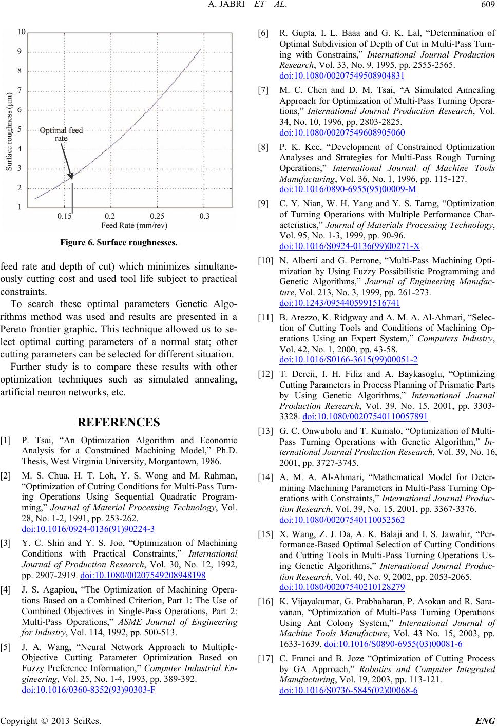

A. JABRI ET AL. 609
Figure 6. Surface roughnesses.
feed rate and depth of cut) which minimizes simultane-
ously cutting cost and used tool life subject to practical
constraints.
To search these optimal parameters Genetic Algo-
rithms method was used and results are presented in a
Pereto frontier graphic. This technique allowed us to se-
lect optimal cutting parameters of a normal stat; other
cutting parameters can be selected for different situation.
Further study is to compare these results with other
optimization techniques such as simulated annealing,
artificial neuron networks, etc.
REFERENCES
[1] P. Tsai, “An Optimization Algorithm and Economic
Analysis for a Constrained Machining Model,” Ph.D.
Thesis, West Virginia University, Morgantown, 1986.
[2] M. S. Chua, H. T. Loh, Y. S. Wong and M. Rahman,
“Optimization of Cutting Conditions for Multi-Pass Turn-
ing Operations Using Sequential Quadratic Program-
ming,” Journal of Material Processing Technology, Vol.
28, No. 1-2, 1991, pp. 253-262.
doi:10.1016/0924-0136(91)90224-3
[3] Y. C. Shin and Y. S. Joo, “Optimization of Machining
Conditions with Practical Constraints,” International
Journal of Production Research, Vol. 30, No. 12, 1992,
pp. 2907-2919. doi:10.1080/00207549208948198
[4] J. S. Agapiou, “The Optimization of Machining Opera-
tions Based on a Combined Criterion, Part 1: The Use of
Combined Objectives in Single-Pass Operations, Part 2:
Multi-Pass Operations,” ASME Journal of Engineering
for Industry, Vol. 114, 1992, pp. 500-513.
[5] J. A. Wang, “Neural Network Approach to Multiple-
Objective Cutting Parameter Optimization Based on
Fuzzy Preference Information,” Computer Industrial En-
gineering, Vol. 25, No. 1-4, 1993, pp. 389-392.
doi:10.1016/0360-8352(93)90303-F
[6] R. Gupta, I. L. Baaa and G. K. Lal, “Determination of
Optimal Subdivision of Depth of Cut in Multi-Pass Turn-
ing with Constrains,” International Journal Production
Research, Vol. 33, No. 9, 1995, pp. 2555-2565.
doi:10.1080/00207549508904831
[7] M. C. Chen and D. M. Tsai, “A Simulated Annealing
Approach for Optimization of Multi-Pass Turning Opera-
tions,” International Journal Production Research, Vol.
34, No. 10, 1996, pp. 2803-2825.
doi:10.1080/00207549608905060
[8] P. K. Kee, “Development of Constrained Optimization
Analyses and Strategies for Multi-Pass Rough Turning
Operations,” International Journal of Machine Tools
Manufacturing, Vol. 36, No. 1, 1996, pp. 115-127.
doi:10.1016/0890-6955(95)00009-M
[9] C. Y. Nian, W. H. Yang and Y. S. Tarng, “Optimization
of Turning Operations with Multiple Performance Char-
acteristics,” Journal of Materials Processing Technology,
Vol. 95, No. 1-3, 1999, pp. 90-96.
doi:10.1016/S0924-0136(99)00271-X
[10] N. Alberti and G. Perrone, “Multi-Pass Machining Opti-
mization by Using Fuzzy Possibilistic Programming and
Genetic Algorithms,” Journal of Engineering Manufac-
ture, Vol. 213, No. 3, 1999, pp. 261-273.
doi:10.1243/0954405991516741
[11] B. Arezzo, K. Ridgway and A. M. A. Al-Ahmari, “Selec-
tion of Cutting Tools and Conditions of Machining Op-
erations Using an Expert System,” Computers Industry,
Vol. 42, No. 1, 2000, pp. 43-58.
doi:10.1016/S0166-3615(99)00051-2
[12] T. Dereii, I. H. Filiz and A. Baykasoglu, “Optimizing
Cutting Parameters in Process Planning of Prismatic Parts
by Using Genetic Algorithms,” International Journal
Production Research, Vol. 39, No. 15, 2001, pp. 3303-
3328. doi:10.1080/00207540110057891
[13] G. C. Onwubolu and T. Kumalo, “Optimization of Multi-
Pass Turning Operations with Genetic Algorithm,” In-
ternational Journal Production Research, Vol. 39, No. 16,
2001, pp. 3727-3745.
[14] A. M. A. Al-Ahmari, “Mathematical Model for Deter-
mining Machining Parameters in Multi-Pass Turning Op-
erations with Constraints,” International Journal Produc-
tion Research, Vol. 39, No. 15, 2001, pp. 3367-3376.
doi:10.1080/00207540110052562
[15] X. Wang, Z. J. Da, A. K. Balaji and I. S. Jawahir, “Per-
formance-Based Optimal Selection of Cutting Conditions
and Cutting Tools in Multi-Pass Turning Operations Us-
ing Genetic Algorithms,” International Journal Produc-
tion Research, Vol. 40, No. 9, 2002, pp. 2053-2065.
doi:10.1080/00207540210128279
[16] K. Vijayakumar, G. Prabhaharan, P. Asokan and R. Sara-
vanan, “Optimization of Multi-Pass Turning Operations
Using Ant Colony System,” International Journal of
Machine Tools Manufacture, Vol. 43 No. 15, 2003, pp.
1633-1639. doi:10.1016/S0890-6955(03)00081-6
[17] C. Franci and B. Joze “Optimization of Cutting Process
by GA Approach,” Robotics and Computer Integrated
Manufacturing, Vol. 19, 2003, pp. 113-121.
doi:10.1016/S0736-5845(02)00068-6

A. JABRI ET AL. 610
[18] U. Zuperl, F. Cus, B. Mursecb and T. Ploj, “A Hybrid
Analytical-Neural Network Approach to the Determina-
tion of Optimal Cutting Conditions,” Journal of Materials
Processing Technology, Vol. 157-158, 2004, pp. 82-90.
doi:10.1016/j.jmatprotec.2004.09.019
[19] X. Wang and I. S. Jawahir, “Optimization of Multi-Pass
Turning Operations Using Genetic Algorithms for the
Selection of Cutting Conditions and Cutting Tools with
Tool-Wear Effect,” International Journal Production
Research, Vol. 43, No. 17, 2005, pp. 3543-3559.
doi:10.1080/13629390500124465
[20] R. Q. Sardinas, M. R. Santana and E. A. Brindis, “Ge-
netic Algorithm-Based Multi-Objective Optimization of
Cutting Parameters in Turning Processes,” Engineering
Applications of Artificial Intelligence, Vol. 19, No. 2,
2006, pp. 127-133. doi:10.1016/j.engappai.2005.06.007
[21] F. Cus and U. Zuperl “Approach to Optimization of Cut-
ting Conditions by Using Artificial Neural Networks,”
Journal of Materials Processing Technology, Vol. 173,
No. 3, 2006, pp. 281-290.
doi:10.1016/j.jmatprotec.2005.04.123
[22] N. R. Abburi and U. S. Dixit, “Multi-Objective Optimiza-
Tion of Multi-Pass Turning Processes,” International
Journal of Advanced Manufacturing Technology, Vol. 32,
No. 9-19, 2007, pp. 902-910.
doi:10.1007/s00170-006-0425-6
[23] A. R. Yildiz, “Hybrid Taguchi-Harmony Search Algo-
rithm for Solving Engineering Optimization Problems,”
International Journal of Industrial Engineering, Vol. 15,
No. 3, 2008, pp. 286-293.
[24] D. K. Ojha, U. S. Dixit and J. P. Davim, “A Soft Com-
puting Based Optimization of Multi-Pass Turning Proc-
esses,” International Journal Material Production Tech-
nology, Vol. 35, No. 1-2, 2009, pp. 145-166.
doi:10.1504/IJMPT.2009.025224
[25] J. Srinivas, R. Giri and S. H. Yang, “Optimization of
Multi-Pass Turning Using Particle Swarm Intelligence,”
International Journal of Advanced Manufacturing Tech-
nology, Vol. 40, 2009, pp. 56-66.
[26] K. Deepak “Cutting Speed and Feed Rate Optimization
for Minimizing Production Time of Turning Process,”
International Journal of Modern Engineering Research,
Vol.2, No. 5, 2012, pp. 3398-3401.
[27] R. Venkata and V. Kalyankar “Multi-Pass Turning Proc-
ess Parameter Optimization Using Teaching-Learning-
Based Optimization Algorithm,” Transactions D: Com-
puter Science & Engineering and Electrical Engineering,
2013 (in press).
[28] A. Aggarwal and H. Singh, “Optimization of Machining
Techniques—A Retrospective and Literature Review,”
Sadhana, Vol. 30, No. 6, 2005, pp. 699-711.
doi:10.1007/BF02716704
[29] K. Deepak “Applications of Different Optimization
Methods for Metal Cutting Operation—A Review,” Re-
search Journal of Engineering Sciences, Vol. 1 No. 3,
2012, pp. 52-58.
[30] E. J. A. Armarego and R. H. Brown, “The Machining of
Metal,” Prentice-Hall, Englewood Cliffs, 1969.
[31] S. K. Hati and S. S. Rao, “Determination of Optimum
Machining Conditions Deterministic and Probabilistic
Approaches,” Journal of Engineering for Industry, Vol.
98, No. 1, 1976, pp. 354-359.
[32] R. V. Narang and G. W. Fischer, “Development of a
Frame Work to Automate Process Planning Functions and
Determine Machining Parameters,” International Journal
of Production Research, Vol. 31, No. 8, 1993, pp. 1921-
1942. doi:10.1080/00207549308956832
[33] D. Goldberg “Genetic Algorithms in Search, Optimiza-
tion, and Machine Learning,” Machine Learning, Vol. 3,
No. 2-3, 1988, pp. 95-99. doi:10.1023/A:1022602019183