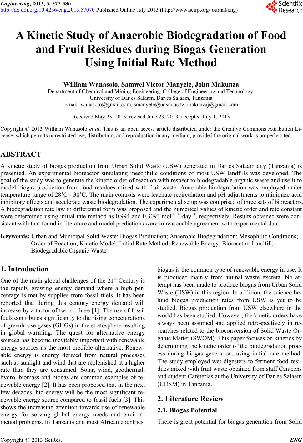
Engineering, 2013, 5, 577-586
http://dx.doi.org/10.4236/eng.2013.57070 Published Online July 2013 (http://www.scirp.org/journal/eng)
A Kinetic Study of Anaerobic Biodegradat ion of Food
and Fruit Residues during Biogas Generation
Using Initial Rate Method
William Wanasolo, Samwel Victor Manyele, John Makunza
Department of Chemical and Mining Engineering, College of Engineering and Technology,
University of Dar es Salaam, Dar es Salaam, Tanzania
Received May 23, 2013; revised June 23, 2013; accepted July 1, 2013
Copyright © 2013 William Wanasolo et al. This is an open access article distributed under the Creative Commons Attribution Li-
cense, which permits unrestricted use, distribution, and reproduction in any medium, provided the original work is properly cited.
ABSTRACT
A kinetic study of biogas production from Urban Solid Waste (USW) generated in Dar es Salaam city (Tanzania) is
presented. An experimental bioreactor simulating mesophilic conditions of most USW landfills was developed. The
goal of the study was to generate the kinetic order of reaction with respect to biodegradable organic waste and use it to
model biogas production from food residues mixed with fruit waste. Anaerobic biodegradation was employed under
temperature range of 28˚C - 38˚C. The main controls were leachate recirculation and pH adjustments to minimize acid
inhibitory effects and accelerate waste biodegradation. The experimental setup was comprised of three sets of bioreactors.
A biodegradation rate law in differential form was proposed and the numerical values of kinetic order and rate constant
were determined using initial rate method as 0.994 and 0.3093 mol0.006·day−1, respectively. Results obtained were con-
sistent with that found in literature and model predictions were in reasonable agreement with experimental data.
Keywords: Urban and Municipal Solid Waste; Biogas Production; Anaerobic Biodegradation; Mesophilic Conditions;
Order of Reaction; Kinetic Model; Initial Rate Method; Renewable Energy; Bioreactor; Landfill;
Biodegradable Organic Waste
1. Introduction
One of the main global challenges of the 21st Century is
the rapidly growing energy demand where a high per-
centage is met by supplies from fossil fuels. It has been
reported that during this century energy demand will
increase by a factor of two or three [1]. The use of fossil
fuels contributes significantly to the rising concentrations
of greenhouse gases (GHGs) in the stratosphere resulting
in global warming. The quest for alternative energy
sources has become inevitably important with renewable
energy sources as the most credible alternative. Renew-
able energy is energy derived from natural processes
such as sunlight and wind that are replenished at a higher
rate than they are consumed. Solar, wind, geothermal,
hydro, biomass and biogas are common examples of re-
newable energy [2]. It has been proposed that in the next
few decades, bio-energy will be the most significant re-
newable energy source compared to fossil fuels [3]. This
shows the increasing attention towards use of renewable
energy for solving global energy needs and environ-
mental problems. In Tanzania and most African countries,
biogas is the common type of renewable energy in use. It
is produced mainly from animal waste excreta. No at-
tempt has been made to produce biogas from Urban Solid
Waste (USW) in this region. In addition, the science be-
hind biogas production rates from USW is yet to be
studied. Biogas production from USW elsewhere in the
world has been studied. However, the kinetic orders have
always been assumed and applied retrospectively in re-
searches related to the bioconversion of Solid Waste Or-
ganic Matter (SWOM). This paper focuses on kinetics by
determining the kinetic order of the biodegradation proc-
ess during biogas generation, using initial rate method.
The study employed wet digesters to ferment food resi-
dues mixed with fruit waste obtained from staff Canteens
and student Cafeterias at the University of Dar es Salaam
(UDSM) in Tanzania.
2. Literature Review
2.1. Biogas Potential
There is great potential for biogas generation from Solid
C
opyright © 2013 SciRes. ENG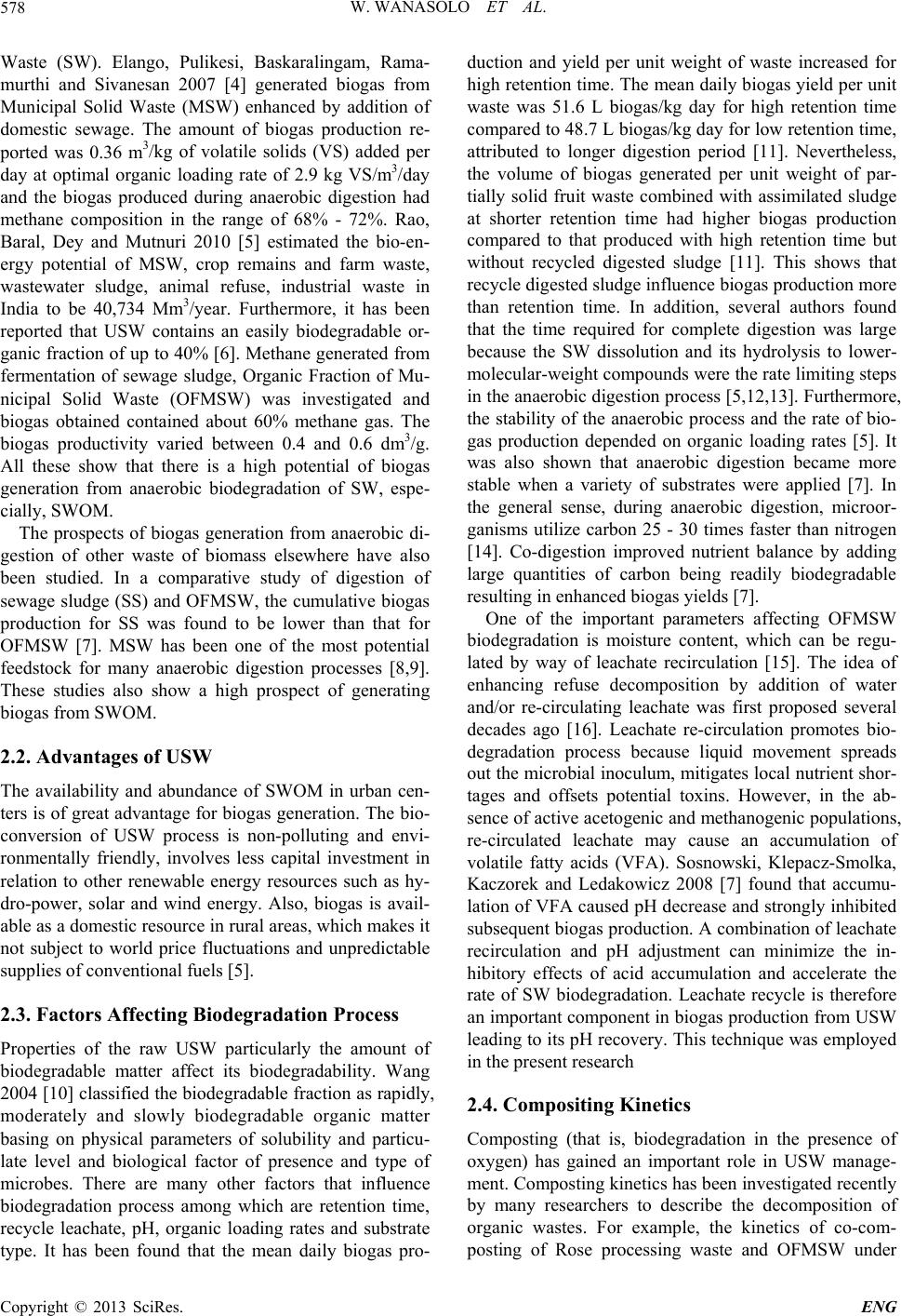

W. WANASOLO ET AL. 578
Waste (SW). Elango, Pulikesi, Baskaralingam, Rama-
murthi and Sivanesan 2007 [4] generated biogas from
Municipal Solid Waste (MSW) enhanced by addition of
domestic sewage. The amount of biogas production re-
ported was 0.36 m3/kg of volatile solids (VS) added per
day at optimal organic loading rate of 2.9 kg VS/m3/day
and the biogas produced during anaerobic digestion had
methane composition in the range of 68% - 72%. Rao,
Baral, Dey and Mutnuri 2010 [5] estimated the bio-en-
ergy potential of MSW, crop remains and farm waste,
wastewater sludge, animal refuse, industrial waste in
India to be 40,734 Mm3/year. Furthermore, it has been
reported that USW contains an easily biodegradable or-
ganic fraction of up to 40% [6]. Methane generated from
fermentation of sewage sludge, Organic Fraction of Mu-
nicipal Solid Waste (OFMSW) was investigated and
biogas obtained contained about 60% methane gas. The
biogas productivity varied between 0.4 and 0.6 dm3/g.
All these show that there is a high potential of biogas
generation from anaerobic biodegradation of SW, espe-
cially, SWOM.
The prospects of biogas generation from anaerobic di-
gestion of other waste of biomass elsewhere have also
been studied. In a comparative study of digestion of
sewage sludge (SS) and OFMSW, the cumulative biogas
production for SS was found to be lower than that for
OFMSW [7]. MSW has been one of the most potential
feedstock for many anaerobic digestion processes [8,9].
These studies also show a high prospect of generating
biogas from SWOM.
2.2. Advantages of USW
The availability and abundance of SWOM in urban cen-
ters is of great advantage for biogas generation. The bio-
conversion of USW process is non-polluting and envi-
ronmentally friendly, involves less capital investment in
relation to other renewable energy resources such as hy-
dro-power, solar and wind energy. Also, biogas is avail-
able as a domestic resource in rural areas, which makes it
not subject to world price fluctuations and unpredictable
supplies of conventional fuels [5].
2.3. Factors Affecting Biodegradation Process
Properties of the raw USW particularly the amount of
biodegradable matter affect its biodegradability. Wang
2004 [10] classified the biodegradable fraction as rapidly,
moderately and slowly biodegradable organic matter
basing on physical parameters of solubility and particu-
late level and biological factor of presence and type of
microbes. There are many other factors that influence
biodegradation process among which are retention time,
recycle leachate, pH, organic loading rates and substrate
type. It has been found that the mean daily biogas pro-
duction and yield per unit weight of waste increased for
high retention time. The mean daily biogas yield per unit
waste was 51.6 L biogas/kg day for high retention time
compared to 48.7 L biogas/kg day for low retention time,
attributed to longer digestion period [11]. Nevertheless,
the volume of biogas generated per unit weight of par-
tially solid fruit waste combined with assimilated sludge
at shorter retention time had higher biogas production
compared to that produced with high retention time but
without recycled digested sludge [11]. This shows that
recycle digested sludge influence biogas production more
than retention time. In addition, several authors found
that the time required for complete digestion was large
because the SW dissolution and its hydrolysis to lower-
molecular-weight compounds were the rate limiting steps
in the anaerobic digestion process [5,12,13]. Furthermore,
the stability of the anaerobic process and the rate of bio-
gas production depended on organic loading rates [5]. It
was also shown that anaerobic digestion became more
stable when a variety of substrates were applied [7]. In
the general sense, during anaerobic digestion, microor-
ganisms utilize carbon 25 - 30 times faster than nitrogen
[14]. Co-digestion improved nutrient balance by adding
large quantities of carbon being readily biodegradable
resulting in enhanced biogas yields [7].
One of the important parameters affecting OFMSW
biodegradation is moisture content, which can be regu-
lated by way of leachate recirculation [15]. The idea of
enhancing refuse decomposition by addition of water
and/or re-circulating leachate was first proposed several
decades ago [16]. Leachate re-circulation promotes bio-
degradation process because liquid movement spreads
out the microbial inoculum, mitigates local nutrient shor-
tages and offsets potential toxins. However, in the ab-
sence of active acetogenic and methanogenic populations,
re-circulated leachate may cause an accumulation of
volatile fatty acids (VFA). Sosnowski, Klepacz-Smolka,
Kaczorek and Ledakowicz 2008 [7] found that accumu-
lation of VFA caused pH decrease and strongly inhibited
subsequent biogas production. A combination of leachate
recirculation and pH adjustment can minimize the in-
hibitory effects of acid accumulation and accelerate the
rate of SW biodegradation. Leachate recycle is therefore
an important component in biogas production from USW
leading to its pH recovery. This technique was employed
in the present research
2.4. Compositing Kinetics
Composting (that is, biodegradation in the presence of
oxygen) has gained an important role in USW manage-
ment. Composting kinetics has been investigated recently
by many researchers to describe the decomposition of
organic wastes. For example, the kinetics of co-com-
posting of Rose processing waste and OFMSW under

W. WANASOLO ET AL. 579
aerobic conditions was evaluated and the results showed
first order kinetics as the best fitting kinetic model [13].
No model has been proposed to fix the kinetic orders for
anaerobic processes of USW. Several other researchers
used first order kinetic models to describe different bio-
degradation processes. Kirchmann and Bernal, 1997 [17]
applied first-zero-order model for aerobic biodegradation
of different material types such as cattle dung, pig dung,
and sewage sludge-cotton waste mixture. Paredes, Bernal,
Cegarra and Roig, 2002 [18] found that organic matter
losses followed a first-order kinetic equation for aerobic
biodegradation of olive mill wastewater sludge. Baptista,
Antunes, Gonçalves, Morvan and Silveira, 2010 [19]
investigated the kinetics of solid waste compositing
based on VS change and the experimental data were fit-
ted with a first-order kinetic model, and a rate constant of
composting under optimum conditions was obtained.
2.5. Modeling Kinetics
Modeling has often been used as the main tool in the
study of composting as well as anaerobic biodegradation
processes, frequently with the aim of optimizing the de-
sign and operation of full-scale plant. Such studies
yielded models such as the Anaerobic Digestion Model
No. 1 (ADM 1) [20] and several other mathematical
models. However, few studies have applied such models
to full scale plants [19]. Besides, Kinetic models for an-
aerobic digestion of organic substrates were derived for
substrate utilization and methane production [21]. The
model equations considered hydrolyzed products as lim-
iting nutrients for microbial growth and biogas produc-
tion according to Monod kinetics. Additionally, a kinetic
model for investigation of the anaerobic digestion of
wastewater generated from orange rind pressing during
orange juice making was proposed basing on the experi-
mental results determined at mesophilic conditions [22].
Monod type kinetic models were also widely used to
describe process kinetics of anaerobic digesters success-
fully [15,23]. Although there was some success in ap-
plying Monod type kinetics to the anaerobic process,
some researchers found it difficult to apply them for their
systems [15,23]. Furthermore, a two-stage model com-
bining zero and first order kinetics based on enzyme re-
action and Monod type micro-organism growth rate
equation was proposed and developed for handling hos-
pital waste biodegradation in landfills [10]. This model
successfully predicted both the cumulative biogas pro-
duction and its rate. It assumed zero order kinetics at the
start of the process followed by a first order kinetics with
respect to biodegradable organic carbon. The model did
not differentiate between the time when the zero order
ends and the start of first order and therefore it was used
ambiguously. Also, Garcı́a-Ochoa, Santos, Naval, Guar-
diola and Lopez, 1999 [12] developed two separate ki-
netic models to explain the anaerobic digestion of live-
stock refuse. This model replicated the experimental data
obtained for cow manure anaerobic digestion with more
accuracy.
In this study, the simulation model developed by
Wang, 2004 [10] was adopted and modified in derivation.
It was assumed that the biodegradation of organic matter
depended on both the amount of biodegradable organic
matter present and moisture content as the primary limit-
ing factors. The model selection was influenced by the
strength of experimental support and mathematical deri-
vations.
3. Methods and Equipment
3.1. Design Features of Experimental Setup
The experimental set-up comprised of three sets of bio-
reactor cells shown in Figure 1. The first set had three
cells in series labeled BA1, BA2 and BA3. The second
had two: BB1 and BB2 and the third had one, BC1. Each
of these cells was of volume 3 liters. Leachate was col-
lected in tanks Lt1, Lt2 and Lt3 and recycled using pumps
P1, P2 and P3, respectively. The pipe system was made of
IPS material to limit corrosion and contamination. Bio-
gas was tapped to the gas measuring device LI1 con-
nected to a calibrated manometer LI2. Using control
valve CV1, the gas volume was measured at regular time
intervals and collected in gas collection bag GB. In gen-
eral a batch type of bioreactors in series was operated at
temperature range of 28˚C - 38˚C.
3.2. Data Collection
Three batches of 12.0, 12.9 and 13.2 kg were prepared at
three different times. Batch one of 12.0 kg was distrib-
uted in six bioreactor cells of Figure 1. Three experi-
ments of weight (Mw) = 6 kg (set one), 4 kg (set two) and
2 kg (set three) each were carried out simultaneously
over a period of about one week. This was repeated for
batches two and three. All the batches comprised of food
residues, fruit waste and non biodegradables shown in
Figure 2.
The SW was sorted and categorized as biodegradable
food residues (BFR), biodegradable fruit waste (BFW)
and non-biodegradable waste (NBW). This categoriza-
tion is shown in Table 1 while Table 2 shows the moles
of biodegradable matter of batches one, two and three. In
the first batch, the different categories of waste were
mixed and distributed in the six bioreactor cells each
taking about 2 kg. Water of pH 7.04 and microbial in-
oculum were added at temperature of 32˚C. The bioreac-
tors were then completely sealed to avoid oxygen inter-
ference and allow mesophilic biodegradation process to
take place. The biogas volume measurements were done

W. WANASOLO ET AL. 580
Figure 1. Experimental Setup: (Lt = Leachate collection tank (10 L), P = Leachate circulation pump (0. 5 Hp), B = Bioreactor
cells (3 L), LI1 = Level Indicator (tank), LI2 = Level Indicator (Manometer), CV1 = Volume control valve and GB = Gas col-
lection bag).
the biodegradation process ceased, indicated by lack of
liquid level displacement at LI2. The pH was restored to
the range of 5.50 to 8.00 by adding leachate after adjust-
ing using Kaoline and also by direct additions of sodium
hydroxide solution. Pumps were switched off to avoid
pump pressure interference with biogas pressure during
volume measurements. The pressure of the system was
brought to zero or atmospheric pressure which was the
reference point for pressure and volume measurements.
Figure 2. Food residues and fruit waste from USDM.
Table 1. Percent composition of food residues mixed with
fruit waste.
Type of waste Batch
One Two Three
BFR 52.50% 53.49% 61.36%
BFW 45.80% 44.19% 37.88%
NBW 1.70% 2.32% 0.76%
Total 100% 100% 100%
3.3. Model Formulation
Table 2. Initial moles of biodegradable waste, nbi
Experimental setup Batch oneBatch two Batch three
1 0.4913 0.5246 0.5578
2 0.3275 0.3497 0.3718
3 0.1638 0.1749 0.1859
Model formulation was based on assumption that the
biodegradation reaction was carried out at standard pres-
sure (atmospheric pressure of 1 atmosphere). However,
the temperature deviated slightly (mesophilic) from stan-
dard conditions. Therefore, the conditions of biodegrade-
tion process were approximated to standard temperature
and pressure. From Avogadro’s law, the volume of 1 mole
of gas at standard temperature and pressure (STP) is
22,400 ml. Therefore, the number of moles of biogas
produced in an experiment, ng, can be determined as per
Equation (1), where Vb = volume of biogas produced in
ml.
22400
b
g
V
n (1)
Using Equation (1), the biogas production rate in 2
minutes sampling time for batches one, two and three
experiments were determined as summarized in Tables
daily for a period of 4 days. After 2 days of biodegrada-
tion, the pH of the reacting matrix dropped significantly
overnight and during the day time to below pH of 4.5 and 3-5, respectively.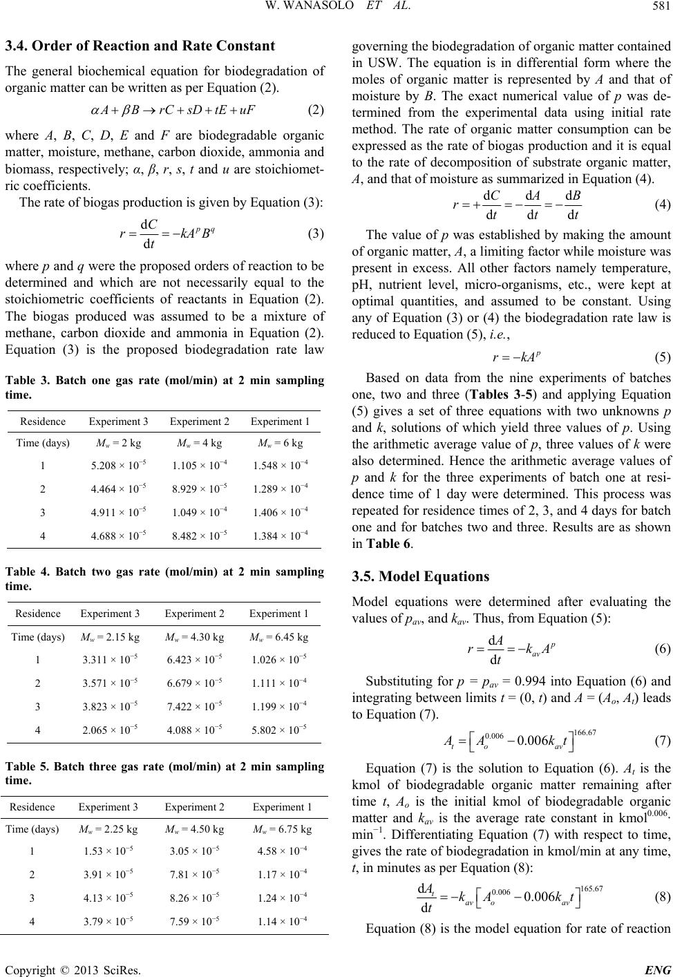

W. WANASOLO ET AL. 581
3.4. Order of Reaction and Rate Constant
ion of
goving the ationattd
in USW. The m
molof orga is r by Aof
The general biochemical equation for biodegradat
organic matter can be written as per Equation (2).
ABrCsD tEuF

  (2)
where A, B, C, D, E and F are biodegrada
matter, moisture, methane, carbon dioxide, a
ble organic
mmonia and
biomass, respectively; α, β, r, s, t and u are stoichiomet-
ric coefficients.
The rate of biogas production is given by Equation (3):
d
d
p
q
C
rkAB
t
 (3)
where p and q were the proposed ord
determined and which are not necessarily equal to the
ers of reaction to be
stoichiometric coefficients of reactants in Equation (2).
The biogas produced was assumed to be a mixture of
methane, carbon dioxide and ammonia in Equation (2).
Equation (3) is the proposed biodegradation rate law
Table 3. Batch one gas rate (mol/min) at 2 min sampling
me. ti
Residence Experiment 3 Experiment 2 Experiment 1
Time (days) M = 2 kg M = 4 kg M = 6 kg
w w w
1 5.208 × 10−5 1.105 × 10−4 1.548 × 10−4
2 4.464 × 10
−58.929 × 10 −51.289 × 10 −4
3 4.911 × 10
−5−4−4
−5−5−4
1.049 × 10 1.406 × 10
4 4.688 × 10 8.482 × 10 1.384 × 10
Table 4. Batche ( 2
me. two gas ratmol/min) atmin sampling ti
Residence Experiment 3 Experiment 2 Experiment 1
Time (days) Mw = 2.15 kg Mw = 4.30 kg Mw = 6.45 kg
1 3.
−5
311 × 10423 × 10026 × 10
−5−5−4
−5−5−5
−56.
−5
−51.
−4
−5
2 3.571 × 10 6.679 × 10 1.111 × 10
3 3.823 × 10 7.422 × 10 1.199 × 10
4 2.065 × 10 4.088 × 10 5.802 × 10
Table 5. Batceng
me. h three gas rat (mol/min) at 2 min sampli ti
Residence Experiment 3 Experiment 2 Experiment 1
Time (days) M = 2.25 kg M = 4.50 kg M = 6.75 kg
w ww
1 1.53 × 10
−5
−53.05 × 10
−5
−54.58 × 10
−4
−4
2 3.91 × 10 7.81 × 10 1.17 × 10
3 4.13 × 10
ernbiodegrad of organic mer containe
equation is in
nic matter
differential for
epresented
where the
and that es
moisture by B. The exact numerical value of p was de-
termined from the experimental data using initial rate
method. The rate of organic matter consumption can be
expressed as the rate of biogas production and it is equal
to the rate of decomposition of substrate organic matter,
A, and that of moisture as summarized in Equation (4).
ddd
ddd
CAB
rttt   (4)
The value of p was established by making the amount
of organic matter, A, a limiting factor whi
present in excess. All other factors namely temperature,
pH
e experiments of batches
one, two and three (Tables 3-5) a
(5) gives a set of three equations
an
tions were determined after evaluating the
, from Equation (5):
le moisture was
, nutrient level, micro-organisms, etc., were kept at
optimal quantities, and assumed to be constant. Using
any of Equation (3) or (4) the biodegradation rate law is
reduced to Equation (5), i.e.,
p
rkA (5)
Based on data from the nin
nd applying Equation
with two unknowns p
d k, solutions of which yield three values of p. Using
the arithmetic average value of p, three values of k were
also determined. Hence the arithmetic average values of
p and k for the three experiments of batch one at resi-
dence time of 1 day were determined. This process was
repeated for residence times of 2, 3, and 4 days for batch
one and for batches two and three. Results are as shown
in Table 6.
3.5. Model Equations
Model equa
values of pav, and kav. Thus
d
d
p
av
A
rkA
t
 (6)
Substituting for p = pav = 0.994 into Equation (6) and
integrating between limits t = (0, t) a
to Equation (7).
s the solution to Equation (6). At is the
kmol of biodegradable organic matter rem
time t, A is the initial kmol of biodegradab
m
nd A = (Ao, At) leads
166.67
0.006 0.006
to av
AA kt



(7)
Equation (7) i
aining after
le organic
o
atter and kav is the average rate constant in kmol0.006·
min−1. Differentiating Equation (7) with respect to time,
gives the rate of biodegradation in kmol/min at any time,
t, in minutes as per Equation (8):
−5−5−4
4 3.79 × 10−5 7.59 × 10−5 1.14 × 10−4
8.26 × 10 1.24 × 10
165.67
0.006
d0.006
d
t
av oav
AkA kt
t
 

(8)
Equation (8) is the model equation for rate of reaction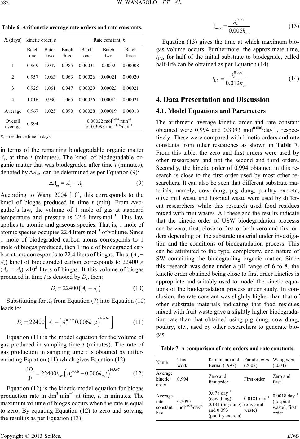

W. WANASOLO ET AL. 582
Table 6. Arithmetic average rate orders and ra
R
te constants.
t (days) kinetic order, p Rate constant, k
Batch
one
Batch
two
Batch
three
Batch
one
Batch
two
Batch
three
1 0.969 1.047 0. 0.00038
Avge
Overall
average
0.006·m −1
06·
985 1 0.0002 0.0000
2 0.957 1.063 0.963 0.00026 0.00021 0.00020
3 0.925 1.061 0.947 0.00029 0.00023 0.00021
4 1.016 0.930 1.065 0.00026 0.00012 0.00021
era0.967 1.025 0.990 0.00028 0.00019 0.00018
0.994 0.0002
or 0.3
2 mol
93 mol0.00
in
day−1
Re d
inorem ining biodegtter
The kmol of biodegradable or-
biodegraded after time t (minutes),
t = residenc time inays.
terms f the aradable organic ma
At, at time t (minutes).
anic matter that wasg
denoted by ∆Aot, can be determined as per Equation (9):
oto t
A
AA (9)
According to Wang 2004 [10], this corresponds to the
kmol of biogas produced in time t (min). From Avo-
gadro’s law, the volume of 1 mole of gas at standard
temperature and pressure is 22.4 liters·mol−1. This law
applies to atomic and gaseous species. That is, 1 mole of
atomic species occupies 22.4 liters·mol−1 of volume. Since
1 mole of biodegraded carbon atoms corresponds to 1
mole of biogas produced, then 1 mole of biodegraded car-
bon atoms corresponds to 22.4 liters of biogas. Thus, (Ao −
At) kmol of biodegraded carbon corresponds to 22400 
(Ao − A
t) 103 liters of biogas. If this volume of biogas
produced in time t is denoted by Dt, then:


22400
tot
DAA
(10)
Substituting for At from Equation (7) into Equation (10)
leads to:

(11) is the model equation for the volume of
gas produced in sampling time t (minutes).
gas production in sampling time t is obtaine
en

166.67
0.006


00
22400 0.006
tav
DAAkt


(11)
Equation
The rate of
d by differ-
tiating Equation (11) which gives Equation (12).

165.67
0.006
d22400 0.006
d
t
av oav
DkA kt
t
(12)
Equation (12) is the kinetic model equation for biogas
production rate in dm3·min−1 at time, t, in min
maximum volume of biogas occurs when the rat
to
th
utes. The
e is equal
zero. By equating Equation (12) to zero and solving,
e result is as per Equation (13):
0.006
max 0.006
o
av
A
tk  (13)
Equation (13) gives the time at which maximum bio-
gas volume occurs. Furthermore, the approximate time,
t1/2, for half of the initial substrate to
half-life can be obtained as per Equation (14).
biodegrade, called
0.006
12 0.012
o
av
A
tk  (14)
4. Data Presentation and Discussion
4.1. Model Equations and Para
The arithmetic average kinetic order and rate constant
1, respec-
ers and rate
in Table 7.
work Bernal (1997) (2002) (2004)
meters
obtained were 0.994 and 0.3093 mol0.006·day−
tively. These were compared with kinetic ord
constants from other researches as shown
From this table, the zero and first orders were used by
other researchers and not the second and third orders.
Secondly, the kinetic order of 0.994 obtained in this re-
search is close to the first order used by most other re-
searchers. It can also be seen that different substrate ma-
terials, namely, cow dung, pig dung, poultry excreta,
olive mill waste and hospital waste were used by differ-
ent researchers while this research used food residues
mixed with fruit wastes. All these and the results indicate
that the kinetic order of USW biodegradation processs
can be zero, first, close to first or both zero and first or-
ders depending on the substrate material under investiga-
tion and the conditions of biodegradation process. This
can be attributed to the type, complexity, and nature of
SW containing the biodegrading organic matter. Since
this research was done under a pH range of 6 to 8, the
kinetic order obtained being close to first order kinetics is
appropriate and suitably used to model the kinetic equa-
tions of the biodegradation process under study. In con-
clusion, the rate constant was slightly higher than that of
other substrate materials indicating that food residues
mixed with fruit waste gave a slightly higher biodegrada-
tion rate than that obtained using pig dung, cow dung,
poultry, etc., used by other researchers to generate bio-
gas.
Table 7. A comparison of rate orders and rate constants.
Name This Kirchmann and Parades et al. Wang et al.
Average
k
or
inetic
der
0.994 Zero and
first order First order Zero and first
Average
·day−1ung)
reta)
ay−1
(olive mill
ay
t
.
rate
constant
kav
0.3093
mol0.006
0.078 day−1
(cow dung),
0.131 (pig d
and 0.093
(poultry exc
0.0181 d
waste)
0.0018 d−1
(hospital
waste), firs
order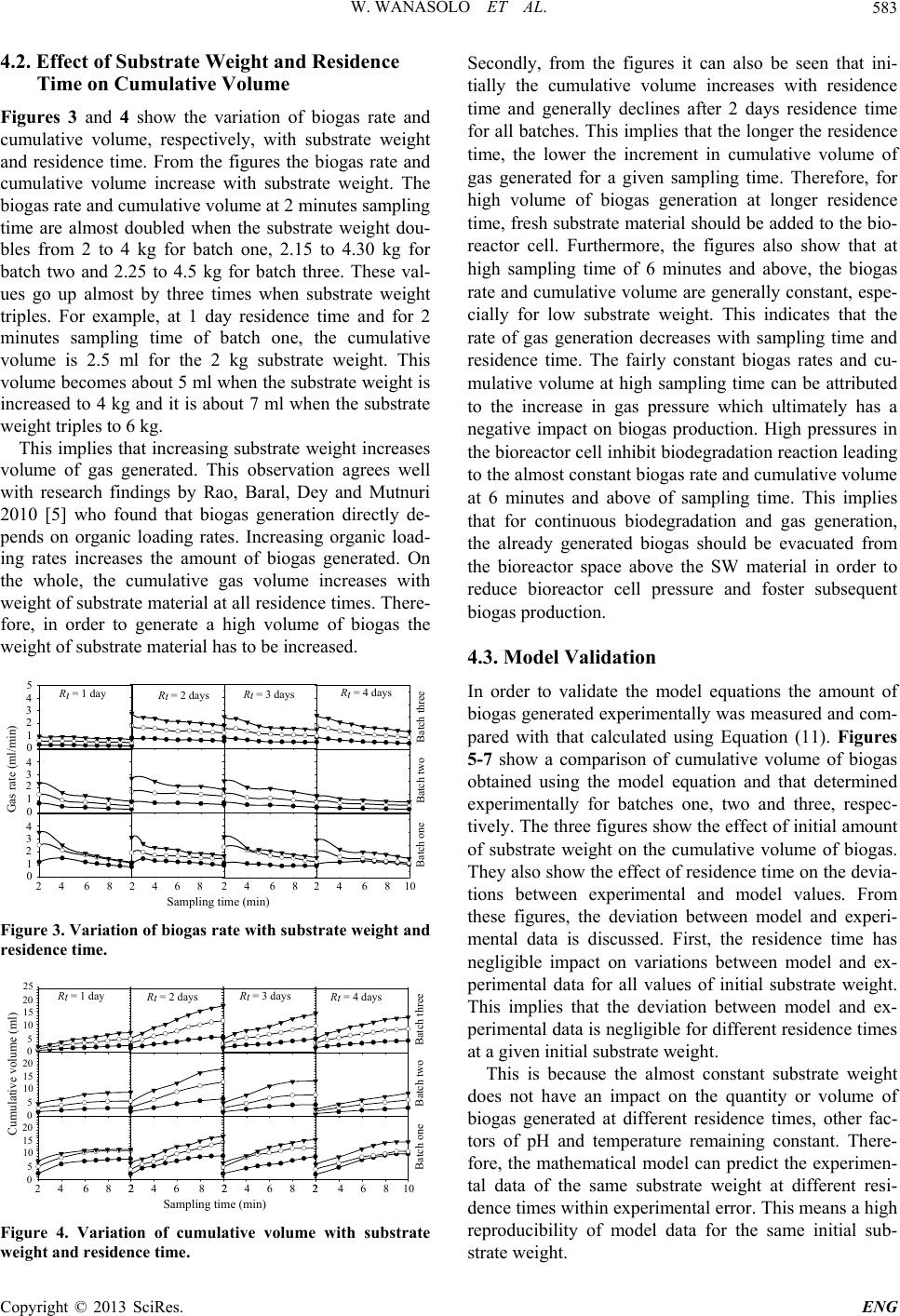

W. WANASOLO ET AL. 583
4.2. Effect of Substrate Weight and Residen
Tim
Figures
ce
s rate and
e on Cu
3 ad 4 sh
m lu
nriatibioga
cumulative volume,with substrate weight
nd
he
biogutes sampling
ulative Vo
ow the va
respectively,
me
on of
and residence time. From the figures the biogas rate a
cumulative volume increase with substrate weight. T
as rate and cumulative volume at 2 min
time are almost doubled when the substrate weight dou-
bles from 2 to 4 kg for batch one, 2.15 to 4.30 kg for
batch two and 2.25 to 4.5 kg for batch three. These val-
ues go up almost by three times when substrate weight
triples. For example, at 1 day residence time and for 2
minutes sampling time of batch one, the cumulative
volume is 2.5 ml for the 2 kg substrate weight. This
volume becomes about 5 ml when the substrate weight is
increased to 4 kg and it is about 7 ml when the substrate
weight triples to 6 kg.
This implies that increasing substrate weight increases
volume of gas generated. This observation agrees well
with research findings by Rao, Baral, Dey and Mutnuri
2010 [5] who found that biogas generation directly de-
pends on organic loading rates. Increasing organic load-
ing rates increases the amount of biogas generated. On
the whole, the cumulative gas volume increases with
weight of substrate material at all residence times. There-
fore, in order to generate a high volume of biogas the
weight of substrate material has to be increased.
Sampling time (min)
Batch one
2 4 6 8 10 2 4 6 8
1
4
2
3
02 4 6 82 4 6 8
Batch two
1
4
3
2
0
Gas rate (ml/min)
Rt = 4 days
Batch three
Rt = 3 days Rt = 2 days
5
1
4
2
3
0
Rt = 1 day
Figure 3. Variation of biogas rate with substrate weight and
residence time.
Sampling time (min)
2 4 6 8 2
0
5
10
15
20
2 4 6 8 22 4 6 8 22 4 6 8 10
Batch oneBatch two
Cumulative volume (ml)
0
5
10
Rt = 4 days
15
20
Batch three
Rt = 3 days
Rt = 2 days
0
5
10
25
15
20
Rt = 1 day
Figure 4. Variation of cumulative volume with substrate
weight and residence time.
Secondly, from the figures it can also be seen that ini-
tially the cumulative volume increases with residence
time and generally declines after 2 days residence time
for all batches. This implies that the longer the residence
time, the lower the increment in cumulative volume of
gas generated for a given sampling time. Therefore, for
high volume of biogas generation at longer residence
time, fresh substrate material should be added to the bio-
reactor cell. Furthermore, the figures also show that at
high sampling time of 6 minutes and above, the bioga
erimental and model values. From
these figures, the deviation between model and experi-
First, the residence time has
s
rate and cumulative volume are generally constant, espe-
cially for low substrate weight. This indicates that the
rate of gas generation decreases with sampling time and
residence time. The fairly constant biogas rates and cu-
mulative volume at high sampling time can be attributed
to the increase in gas pressure which ultimately has a
negative impact on biogas production. High pressures in
the bioreactor cell inhibit biodegradation reaction leading
to the almost constant biogas rate and cumulative volume
at 6 minutes and above of sampling time. This implies
that for continuous biodegradation and gas generation,
the already generated biogas should be evacuated from
the bioreactor space above the SW material in order to
reduce bioreactor cell pressure and foster subsequent
biogas production.
4.3. Model Validation
In order to validate the model equations the amount of
biogas generated experimentally was measured and com-
pared with that calculated using Equation (11). Figures
5-7 show a comparison of cumulative volume of biogas
obtained using the model equation and that determined
experimentally for batches one, two and three, respec-
tively. The three figures show the effect of initial amount
of substrate weight on the cumulative volume of biogas.
They also show the effect of residence time on the devia-
tions between exp
mental data is discussed.
negligible impact on variations between model and ex-
perimental data for all values of initial substrate weight.
This implies that the deviation between model and ex-
perimental data is negligible for different residence times
at a given initial substrate weight.
This is because the almost constant substrate weight
does not have an impact on the quantity or volume of
biogas generated at different residence times, other fac-
tors of pH and temperature remaining constant. There-
fore, the mathematical model can predict the experimen-
tal data of the same substrate weight at different resi-
dence times within experimental error. This means a high
reproducibility of model data for the same initial sub-
strate weight.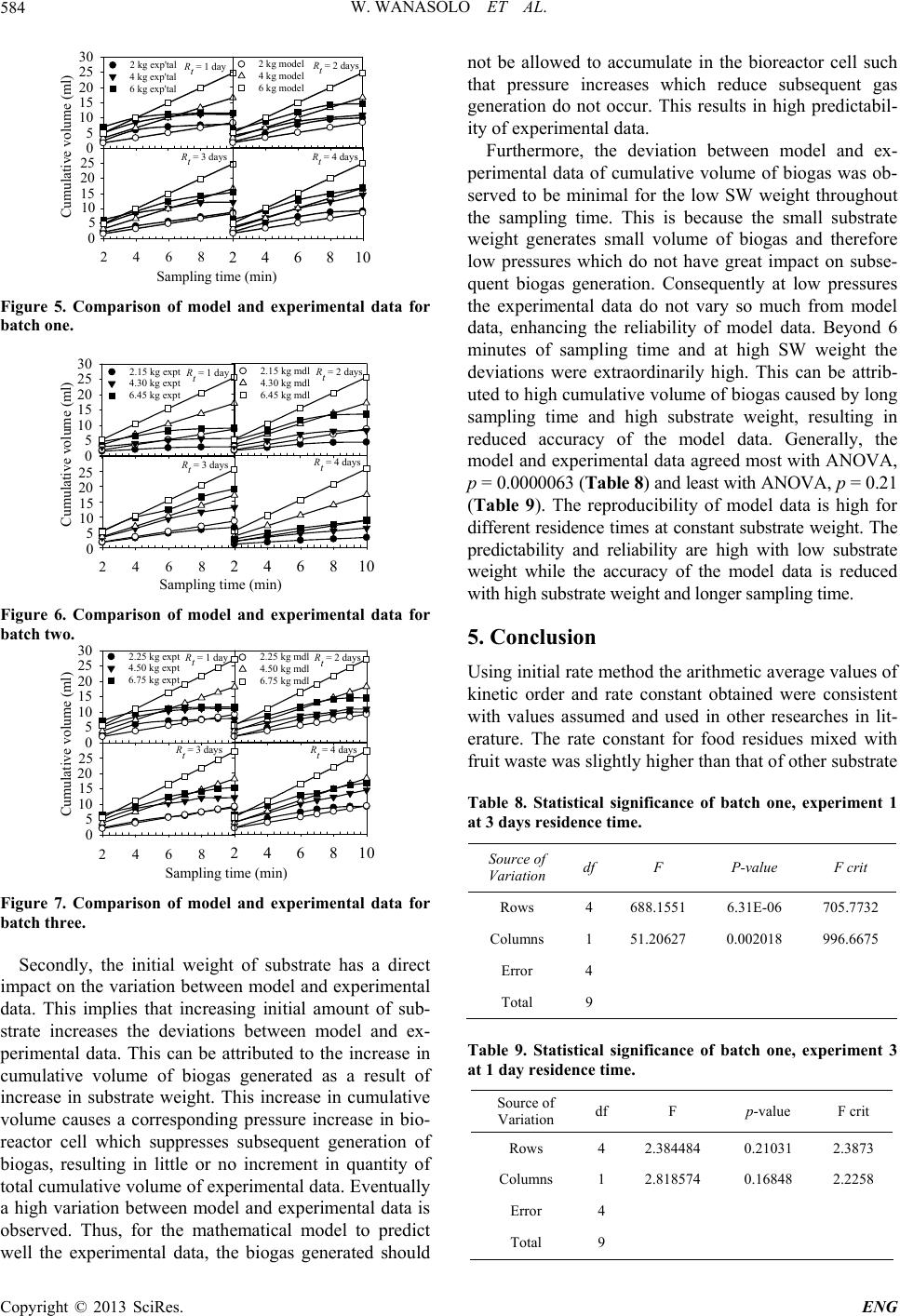

W. WANASOLO ET AL. 584
Rt = 1 day
0
5
10
15
20
25
30
4 kg exp'tal
6 kg exp'tal
2 kg exp'tal
Rt = 3 days
Sampling time (min)
Cumulative volume (ml)
0
5
10
15
20
25
2 4 6 8
Rt = 4 days
246810
Rt = 2 days
2 kg model
4 kg model
6 kg model
Figure 5. Comparison of model and experimental data for
batch one.
Rt = 1 day
0
5
10
15
20
25
30
2.15 kg expt
4.30 kg expt
6.45 kg expt
Rt = 2 days
2.15 kg mdl
4.30 kg mdl
6.45 kg mdl
Rt = 4 days
24681
0
Rt = 3 days
Sampling time (min)
Cumulative volume (ml)
2 4 6 8
0
5
10
15
20
25
Figure 6. Comparison of model and experimental data for
atch two. b
Rt = 2 days
2.25 kg mdl
4.50 kg mdl
6.75 kg mdl
Rt = 1 day
0
5
10
15
20
25
30
2.25 kg expt
4.50 kg expt
6.75 kg expt
Rt = 4 days
24681
0
Rt = 3 days
Sampling time (min)
Cumulative volume (ml)
2 4 6 8
0
5
10
15
20
25
Figure 7. Comparison of model and experimental data for
batch three.
Secondly, the initial weight of substrate has a direct
impact on the variation between model and experimental
data. This implies that increasing initial amount of sub-
strate increases the deviations between model and ex-
perimental data. This can be attributed to the increase in
cumulative volume of biogas generated as a result of
increase in substrate weight. This increase in cumulative
volume causes a corresponding pressure increase in bio-
reactor cell which suppresses subsequent generation of
biogas, resulting in little or no increment in quantity of
bserved. Thus, for the mathematical model to predict
well the experimental data, the biogas generated should
no
model data. Generally, the
m
total cumulative volume of experimental data. Eventually
a high variation between model and experimental data is
o
t be allowed to accumulate in the bioreactor cell such
that pressure increases which reduce subsequent gas
generation do not occur. This results in high predictabil-
ity of experimental data.
Furthermore, the deviation between model and ex-
perimental data of cumulative volume of biogas was ob-
served to be minimal for the low SW weight throughout
the sampling time. This is because the small substrate
weight generates small volume of biogas and therefore
low pressures which do not have great impact on subse-
quent biogas generation. Consequently at low pressures
the experimental data do not vary so much from model
data, enhancing the reliability of model data. Beyond 6
minutes of sampling time and at high SW weight the
deviations were extraordinarily high. This can be attrib-
uted to high cumulative volume of biogas caused by long
sampling time and high substrate weight, resulting in
reduced accuracy of the
odel and experimental data agreed most with ANOVA,
p = 0.0000063 (Table 8) and least with ANOVA, p = 0.21
(Table 9). The reproducibility of model data is high for
different residence times at constant substrate weight. The
predictability and reliability are high with low substrate
weight while the accuracy of the model data is reduced
with high substrate weight and longer sampling time.
5. Conclusion
Using initial rate method the arithmetic average values of
kinetic order and rate constant obtained were consistent
with values assumed and used in other researches in lit-
erature. The rate constant for food residues mixed with
fruit waste was slightly higher than that of other substrate
Table 8. Statistical significance of batch one, experiment 1
at 3 days residence time .
Source of
Variation df F P-value F crit
Rows 4 688.1551 6.31E-06 705.7732
Columns 1 51.20627 0.002018 996.6675
Error 4
Total 9
Table 9. Statistical significance of batch one, experiment 3
at 1 day residence time.
Source of
Variation dfF p-value F crit
Rows 4 2.384484 0.21031 2.3873
Columns 1 2.8574 8
Total 9
810.1684 2.2258
Error 4

W. WANASOLO ET AL. 585
maplyg aggrade
than obtainng pig dung, cow dung, poultr
usedher researchers to generate ogas. This i
portnsidrenewable energy sources for im
roved efficiencies and yield. The cumulative gas
idence times. In order to gen
a hie of biogas the weight of substrate material
hascreased. Alsor high volud
high tion e atsidee, fb-
straterial shold beo thctor
for us bdegandnerae
alreaneratebiogas ould be removed fro the
bioreactor in order to ena le more biogas production.
Biotechnology, Vo
85, No. 4, 2010, pp. 849-860.
246-7
terials imin slightly hiher biodeation rat
that
by ot
ed usiy, etc.,
s im-bi
ant coering -
vop l-
ume and gas generation rate increase with weight of sub-
strate material at all reserate
gh volum
to be in, fo biogasme an
genera
mate
rat
u
longer re
added t
nce tim
e biorea
resh su
cell and
continuoioradation gas getion, th
dy ged shm
b
Increasing the substrate weight increased the absolute
deviation, absolute mean and standard deviations, attrib-
uted to the increase in biogas pressure caused by cumula-
tive gas volume in the manometer. The longer the resi-
dence time the lower the absolute deviation, absolute
mean and standard deviations, attributing to the low gas
pressure due to low cumulative volume. The model pre-
dicted well the experimental data for low substrate weight
at all residence times and for high substrate weight at
longer residence time. For the model which has predicted
well the experimental data at higher substrate weight and
shorter residence time, the biogas generated should have
been removed from the bioreactor cell immediately when
it is formed. It would be helpful to pursue further re-
search about the study and experimental design consid-
ering detaching the cumulative volume measuring unit
from the bioreactor cell thereby eliminating biogas ac-
cumulation within the bioreactor cell.
6. Acknowledgements
The success of this work has been made possible with
financial assistance from Kyambogo University, Uganda
and University of Dar es Salaam, Tanzania.
REFERENCES
[1] OECD/IEA, “World Energy Outlook, International En-
ergy Agency,” OECD/IEA, Paris, 2006.
[2] OECD/IEA, “Working Together to Ensure Reliable, Af-
fordable and Clean Energy, International Energy
Agency,” 2012,
[3] P. Weiland, “Biogas Production: Current State and Per-
spectives,” Applied Microbiology andl.
doi:10.1007/s00253-009-2
007, pp. 301-
304. doi:10.1016/j.jhazmat.2006.07.003
[4] D. Elango, M. Pulikesi, P. Baskaralingam, V. Rama-
murthi and S. Sivanesan, “Production of Biogas from
Municipal Solid Waste with Domestic Sewage,” Journal
of Hazardous Materials, Vol. 141, No. 1, 2
[5] P. V. Rao, S. . Mutnuri, “Biogas
o. 7, 2010, pp.
S. Baral, R. Dey and S
Generation Potential by Anaerobic Digestion for Sus-
tainable Energy Development in India,” Renewable and
Sustainable Energy Reviews, Vol. 14, N
2086-2094. doi:10.1016/j.rser.2010.03.031
[6] P. Sosnowski, A. Wieczorek and S. Ledakowicz, “An-
aerobic Co-Digestion of Sewage Sludge and Organic
49-7
Fraction of Municipal Solid Wastes,” Advances in Envi-
ronmental Research, Vol. 7, No. 3, 2003, pp. 609-616.
doi:10.1016/S1093-0191(02)000
a, K. Kaczorek and S. [7] P. Sosnowski, A. Klepacz-Smolk
Ledakowicz, “Kinetic Investigations of Methane Co-
Fermentation of Sewage Sludge and Organic Fraction of
Municipal Solid Wastes,” Bioresource Technology, Vol.
99, No. 13, 2008, pp. 5731-5737.
doi:10.1016/j.biortech.2007.10.019
[8] K. Braber, “Anaerobic Digestion of Municipal Solid
Waste: A Modern Waste Disposal Option on the Verge of
Breakthrough,” Biomass and Bioenergy, Vol. 9, No. 1-5,
1995, pp. 365-376. doi:10.1016/0961-9534(95)00103-4
[9] A. Ambulkar and A. Shekdar, “Prospects of Biomethana-
tion Technology in the Indian Context: A Pragmatic Ap-
proach,” Resources, Conservation and Recycling, Vol. 40,
No. 2, 2004, pp. 111-128.
doi:10.1016/S0921-3449(03)00037-5
[10] Q. Wang, “Aspects of Pretreated Hospital Waste Biodeg-
s Production and Its
d Management, Vol.
radation in Landfills,” Department of Mechanical Engi-
neering, University of Duisburg-Essen, Essen, 2004.
[11] G. Lastella, C. Testa, G. Cornacchia, M. Notornicola, F.
Voltasio and V. K. Sharma, “Anaerobic Digestion of
Semi-Solid Organic Waste: Bioga
Purification,” Energy Conversion an
43, No. 1, 2002, pp. 63-75.
doi:10.1016/S0196-8904(01)00011-5
[12] F. Garcı́a-Ochoa, V. Santos, L. Naval, E. Guardiola and B.
Lopez, “Kinetic Model for Anaerobic Digestion of Live-
stock Manure,” Enzyme and Microbial Technology, Vol.
25, No. 1-2, 1999, pp. 55-60.
doi:10.1016/S0141-0229(99)00014-9
[13] I. Tosun, M. Gönüllü, E.
“Co-Composting Kinetics of Rose Pro
Arslankaya and A. Günay,
cessing Waste with
Organic Fraction of Municipal Solid Waste,” Bioresource
Technology, Vol. 99, No. 14, 2008, pp. 6143-6149.
doi:10.1016/j.biortech.2007.12.039
[14] T. Sreekrishnan, S. Kohli and V. Rana, “Enhancement of
Biogas Production from Solid Substrates Using Different
Techniques—A Review,” Bioresource Technology, Vol.
95, No. 1, 2004, pp. 1-10.
doi:10.1016/j.biortech.2004.02.010
002/bit.10450
[15] V. Vavilin, S. Rytov, L. Lokshina, S. Pavlostathis and M.
Barlaz, “Distributed Model of Solid Waste Anaerobic
Digestion: Effects of Leachate Recirculation and pH Ad-
justment,” Biotechnology and Bioengineering, Vol. 81,
No. 1, 2003, pp. 66-73. doi:10.1
Stabilization with
Bio-
[16] F. G. Pohland, “Sanitary Landfill
Leachate Recycle and Residual Treatment, Epa,” Civil
Engineering, Vol. 106, No. 6, 1975, pp. 1057-1069
[17] H. Kirchmann and M. Bernal, “Organic Waste Treatment
and C Stabilization Efficiency,” Soil Biology and

W. WANASOLO ET AL. 586
pp. 1747-1753. chemistry, Vol. 29, No. 11-12, 1997,
doi:10.1016/S0038-0717(97)00065-5
[18] C. Paredes, M. Bernal, J. Cegarra and A. Roig, “Bio-
Degradation of Olive Mill Wastewater Sludge by Its
Co-Composting with Agric
Technology, Vol. 85, No. 1, 2002, pp
ultural Wastes,” Bioresource
. 1-8.
doi:10.1016/S0960-8524(02)00078-0
[19] M. Baptista, F. Antunes, M. S. Gonçalves, B. Morvan and
A. Silveira, “Composting Kinetics in Full-Scale Me-
chanical-Biological Treatment Plants,” Waste Manage-
ment, Vol. 30, 2010, pp. 1908-1921.
[20] R. K. Dereli, M. E. Ersahin, H. Ozgun, I. Ozturk and A. F.
Aydin, “Applicability of Anaerobic Digestion Model No.
1 (Adm1) for a Specific Industrial Wastewater: Opium
Alkaloid Effluents,” Chemical Engineering Journal, Vol.
165, No. 1, 2010, pp. 89-94.
doi:10.1016/j.cej.2010.08.069
[21] A. Barthakur, M. Bora and H. D. Singh, “Kinetic Model
for Substrate Utilization and Methane Production in the
Anaerobic Digestion of Organic Feeds,” Biotechnology
Progress, Vol. 7, 1991, pp. 369-376.
doi:10.1021/bp00010a012
[22] J. Siles, M. Martin, A. Chica and R. Borja, “Kinetic Mod-
elling of the Anaerobic Digestion of Wastewater Derived
from the Pressing of Orange
Juice Manufacturing,” Chemi
Rind Produced in Orange
cal Engineering Journal,
Vol. 140, No. 1-3, 2008, pp. 145-156.
doi:10.1016/j.cej.2007.09.026
[23] K. P. Singh, S. Gupta, A. K. Singh and S. Sinha, “Opti-
mizing Adsorption of Crystal Violet D
Magnetic Nanocomposite U
ye from Water by
sing Response Surface Mod-
eling Approach,” Journal of Hazardous Materials, Vol.
186, 2011, pp. 1462-1473.