Journal of Modern Physics, 2013, 4, 85-95
http://dx.doi.org/10.4236/jmp.2013.47A1010 Published Online July 2013 (http://www.scirp.org/journal/jmp)
Dark Particles Answer Dark Energy
John L. Haller Jr.
Predictive Analytics, CCC Information Services, Chicago, USA
Received April 11, 2013; revised May 13, 2013; accepted June 15, 2013
Copyright © 2013 John L. Haller Jr. This is an open access article distributed under the Creative Commons Attribution License,
which permits unrestricted use, distribution, and reproduction in any medium, provided the original work is properly cited.
ABSTRACT
This paper argues that a hypothetical “dark” particle (a black hole with the reduced Planck mass and arbitrary tempera-
ture) gives a simple explanation to the open question of dark energy and has a relic density of only 17% more than the
commonly accepted value. By considering an additional near-horizon boundary of the black hole, set by its quantum
length, the black hole can obtain an arbitrary temperature. Black-body radiation is still present and fits as the source of
the Universe’s missing energy. Support for this hypothesis is offered by showing that a stationary solution to the black
hole’s length scale is the same if derived from a quantum analysis in continuous time, a quantum analysis in discrete
time, or a general relativistic analysis.
Keywords: Dark Particle; Dark Energy; Black Hole; Black-Body Radiation; Diffusion; Brownian Motion; Langevin
Equation; Dark Matter
1. Introduction
Cosmological observations from early in the last century
indicate the Universe is expanding. These observations
show that the speed at which objects move away from
Earth has a strong correlation with their distance, known
as Hubble’s Law. However, it was not until the end of
the last century, when we had observations of Type Ia
supernova, that we concluded the Universe is also accel-
erating [1].
The most popular explanation for these findings is an
elusive energy density with an equation of state, w <
−1/3 [2] coined “Dark Energy” making up ~73% [3] of
the energy density of the Universe. Many attempts have
been made to explain dark energy’s origin [4], yet those
attempts have ultimately been unsatisfying [2,5]. Many
theories are still under review [6,7]; with the most ac-
cepted being the Lambda Cold Dark Matter model,
ΛCDM where Lambda, the Cosmological Constant, pro-
vides a negative pressure , to the Universe [1,2]. 1w
1w
By hypothesizing a “dark particle” we begin to answer
the question of the missing dark energy density. We will
see that a dark particle is a black hole with the reduced
Planck mass. At this mass, the original assumption in
Hawking’s work on black hole radiation [8] breaks down
and I show how a quantum boundary, set by the width of
the wave packet, is larger than the event horizon. The
surface gravity at this new quantum boundary is such that
the temperature is arbitrary. Still the distribution of ki-
netic and potential energy is shown to be that of the
black-body.
We now have a source of a black-body energy density
that contributes to the energy density of the Universe.
One might conclude that dark particles are in thermal
equilibrium with the Cosmic Microwave Background;
however, I will argue that the coupling mechanism be-
tween the dark particles and the background radiation
field has been turned off since after the Dark Ages when
re-ionization happened. If this is the case and if the dark
particles temperature is frozen, they have an equation of
state of

 and the right relic density to explain
dark energy.
It is also shown how the dark particles cool via a sta-
tionary diffusive process where the quantum solution to
width of the wave packet (the near horizon quantum
boundary) is derived. I present this analysis in both con-
tinuous and discrete space-time and use a computer model
to show that the two give the same solution. A linkage
between quantum mechanics and gravity is gained by
considering three energy density terms of the dark parti-
cle. The resulting length scale, as solved by Friedmann’s
equation, is identical to solution of its quantum length.
Section 2 argues that a black hole with the reduced
Planck mass (a dark particle) has an arbitrary tempera-
ture and that its density explains dark energy. Section 3
confirms that a dark particle’s energy is still in the form
C
opyright © 2013 SciRes. JMP

J. L. HALLER JR. 86
of black-body radiation. Section 4 solves the length scale
of a dark particle from a continuous quantum derivation
and explains the mechanism by which the dark particle
cools. Section 5 validates the solution to the length scale
derived in Section 4 by modeling the diffusive process in
discrete space-time. Section 6 shows that an identical
solution to the length scale can also be derived from
Friedmann’s equation when appropriate densities are con-
sidered. Section 7 discusses other similar work and how
dark particles might solve other open questions as well,
such as dark matter.
2. Missing Energy
2.1. Dual Gaussians
We begin by setting the context on a particle of mass m
in equilibrium with a heat bath at temperature T. We as-
sume a particle is in the dual Gaussian ground state.



2
2
0
2Δ
2e
x
x
0
1
~
2Δ
x
px dxx 
dx

 (1)
 

2
2
0
2Δ
e
x
p
p
2
0
1
~
2Δ
x
xx
pppdp p x dp



2
0B
(2)
Using the equipartition theorem on the kinetic energy
[9], one has
Δ
p
mk T

(3)
And using Heisenberg’s Uncertainty equation [9],

22
2
04B
mk T

 2
0
Δ
4Δ
xp  (4)
Making use of the equipartition theorem implies that
the particle is coupled to an ensemble of particles or heat
bath [10]. The bath in this case is an external radiation
field (for example, the Cosmic Microware Background).
However, as we will see, the coupling between the dark
particles and the heat back can be turned on or off with
the presence or absence of neutral hydrogen atoms. We
will use the temperature at the time of last coupling and
the particle’s mass to define the width of the wave func-
tion.
2.2. Black Holes
We will now apply these lengths to our understanding of
black holes, specifically holes with a mass equal to the
reduced Planck mass.
8
c
mG 
 (5)
A number of special conditions arise at this value of
mass. First, the quantum limit, 2dx mc is equal to a
circle’s circumference with the Schwarzschild radius,
Figure 1.
24
2S
dxR Gm
mc  (6)
Indeed this is a small cross-sectional area for the black
hole.
Second, the Hawking temperature is equal to the mass
of the black hole,

3
262
Hawking 4.3 10grams
8
Bc
kT mcc
Gm





5
10 g

(7)
Third, it is not clear that the Hawking temperature is
valid at this value of the mass. Specifically Hawking
stated in his seminal paper from 1975 [8], “Eventually,
when the mass of the black hole is reduced to ,
the quasi-stationary approximation will break down. At
this point, one cannot continue to use the concept of a
classical metric. However, the total mass or energy re-
maining in the system is very small.”
Even more recent derivations of Hawking’s work still
breakdown at this mass [11]. I will argue that when a
black hole has the reduced Planck mass, the Hawking
temperature breaks down because a secondary quantum
boundary is greater than the Schwarzschild radius and it
is this boundary that defines the near horizon’s surface
gravity. The length of the boundary is such that its sur-
face gravity/temperature is arbitrary. I will also argue
that even though “the total energy in the system is very
small,” it has just the right density (given the history of
our Universe) to explain dark energy.
2.3. Quantum Boundary
As the event horizon is defined by the quantum limit, dx,
the outer quantum boundary is defined by the square root
of the position’s variance 

0
Δ
x
. If 0 Δ
x
defines the
circumference of the boundary (as defines the cir-
cumference of the event horizon), the radius of the outer
boundary will be , see Figure 1.
dx
QB
R
RS
dx
RQB Δx
Figure 1. Event horizon (solid line) and quantum boundary
(dotted line) of dark particle.

J. L. HALLER JR. 87
Nocoupling
mechanism
0
QB
Δ
2π
x
R4πB
mk T

r
(8)
The surface gravity at radius is [12],

222
Gm Gm
cr cr




QB
R
12
1
2
rr





 (9)
The effective temperature [8] for surface gravity at ra-
dius will thus be,

2
8πGm T
TT
c 
R
QB
DarkParticle 2πB
R
kc



(10)
The width of the black hole’s wave packet (which is
set by the temperature of the heat bath) that defines the
outer quantum boundary is just the right size to define a
surface gravity such that the temperature is arbitrary and
not a function of mass or other defining feature of the
black hole. The temperature is its own independent pa-
rameter of the black hole. Thus I will call a black hole
with the reduced Planck mass and arbitrary temperature a
dark particle.
ω
2
Couplingmechanism
thro u gh hydrogenatoms
Hydrogenatoms
ω
1
When the mass of a black hole is greater than the re-
duced Planck mass, the quantum boundary QB is nec-
essarily smaller than RSchwarzschild and thus it is RSchwarzschild
that defines the surface gravity. When the black hole is a
dark particle it can’t lose any more mass lest its quantum
limit will become larger than RSchwarzschild; thus it will
cease to be a black hole. If the dark particle loses radia-
tion it must shed its non-massive energy and thus de-
crease in temperature. On the flip side, if the dark parti-
cle is in a heat bath at a higher temperature than the dark
particle, it will match that larger temperature (assuming a
coupling mechanism is in place) without gaining mass
until the reduced Planck temperature is reached.
2.4. Dark Energy
Now hypothesize that a local group of dark particles are
able to exchange heat with the Cosmic Microwave Back-
ground wh en neutral hydrogen atoms or other sinks are
nearby to capture the radiation from its gravitational
binding but that th ey become frozen (constant tempera-
ture) when neutral hydrogen atoms are not nearby.
This hypothesis rests on the idea that a virtual particle
that leaves its pair becomes trapped by the outer quantum
boundary, even if it escapes the event horizon, unless a
sink is around to capture it. See Figure 2. With no sink
the net energy to escape is zero. However if a sink is
around, like a neutral hydrogen atom, the sink can absorb
radiation at one energy and release radiation into the dark
particle at another energy, keeping it in thermal equilib-
rium.
During the dark ages, the time between decoupling and
re-ionization [13], the Universe was filled with hydrogen
Figure 2. Without a coupling mechanism, the radiation
can’t escape thereby not allowing the dark particle to cool.
However with a hydrogen atom or other sink the dark par-
ticle can equilibrate with the background field.
atoms that provided the coupling mechanism between the
dark particles and regular energy. In these conditions the
dark particles were coupled to the Cosmic Microwave
Background (CMB). However after re-ionization, the
hydrogen was ionized and the dark particles and its asso-
ciated radiation energy density became frozen. The
red-shift of re-ionization and the current temperature of
the CMB provide an estimate of the temperature of the
dark particles at the time of re-ionization where it re-
mains constant up to today.


DPRe-ionization CMB-today
1 constantTz T (11)
If we know the temperature of the dark particles at
re-ionization, then we should have an idea for the total
energy density that contributes to the Cosmological con-
stant today.

4
2
Dark Particles-BBR35
15
BDP
kT
c



D
(12)
Because we have estimates of today’s z value of re-
ionization and today’s temperature of the CMB we can
estimate the density, P-BBR

. The Lambda Cold Dark
Matter model, , provides a completely inde-
pendent estimate of the density of dark energy, Λ
ΛCDM
CDM

[1], which we can estimate using the parameter, ,
and today’s Hubble constant.
Λ
Ω
2
ΛΛcritical Λ
3
ΩΩ
8
CDM
H
G
  
 (13)

J. L. HALLER JR. 88
Using the 7-year Wilkinson Microwave Anisotropy
Probe [3] as a source for our estimates Table 1 and Fig-
ure 3 show how our model’s estimate of dark energy is
higher by 17% but well within the confidence range de-
fined by .
re-ionization
z
34
~10
26
0
2.5. Inflation
It is also supportive to examine how this theory holds up
to the inflationary period just after the big bang. The in-
flationary period that follows the grand unified period
lasts for seconds and during this time, the scale
factor of the Universe grows exponentially by a factor of
[14]. Assuming that dark particles are able to
release heat, thereby maintaining equilibrium with the
rest of the Universe’s energy during the time of grand
unification (immediately preceding inflation), but that
once the inflation period began the dark particles became
isolated,then the dark particles will have a constant en-
ergy density during inflation leading to exponential ex-
pansion (but with a much higher rate than today).
~1
The theory also provides insights into reheating, the
period after inflation. If you imagine the dark particles
were at the temperature of grand unification at the begin-
ning of the inflationary epoch only to become isolated,
Table 1. Estimate and confidence ranges of Dark Energy
from the Dark Particles BBR model and the Lambda Cold-
Dark Matter model using 7-year WMAP data.
Low Average High
DP BBR




3
kg m 5.22E−27 8.12E−27 1.21E−26
today
T


degrees
re-ionization
z
CDM


2.725 2.725 2.725
9.3 10.5 11.7


3
kg m
H
6.21E−27 6.95E−27 7.74E−27

km sec Mpc


68.5 71.0 73.5
0.705 0.734 0.763
4.0 6.0 8.0 10.012.014.01e‐27kg/m
ρ(Dark Particles’BBR)
ρ(ΛCDM)
2
PE Cx
3
Figure 3. Visualization of density of dark energy from two
models.
the dark particles would remain constant during the infla-
tion while the rest of the energy density in the Universe
would cool by a factor of ~(1026)4. If quarks, anti-quarks
or gluons (which became available at the end of the in-
flationary period) are able to couple dark particles to the
rest of the Universe’s energy (as we hypothesized neutral
hydrogen atoms are able to do), heat could flow from the
hot dark particles back into the rest of the Universe, re-
heating it.
3. Black-Body Radiation
With the derivation of the Hawking temperature breaking
down at the reduced Planck mass, the derivation of
black-body radiation is also in question. However as we
see below, a black hole with the reduced Planck mass
and arbitrary temperature still radiates a density of en-
ergy with the black-body distribution.
3.1. Resistive Force
We begin by assuming aquadratic potential energy term.
If the equipartition theorem and Heisenberg Uncertainty
principle hold [9] we can derive the potential energy term.
We have for one dimension,
(14)
From the equipartition theorem,
2
B
kT
PE KE (15)
2
2
22
B
kT
p
Cx m
 (16)
If 0xp

 and if 02px

, one can deduce
the potential energy and the associated force
2
2
2
mx
PE  (17)

2
mx
F


 (18)
where,
2B kT. (19)



In Section 4 we show how this force is related to ki-
netic motion. Further in Section 6 we show this resistive
force can also be derived from the self-gravitational po-
tential of the particle and thus only acts over the distance
defined by the Schwarzschild radius. Since the Sch-
warzschild radius is much smaller than the quantum step
size of any particle we have experimental data on, we
have never directly observed this effect.

J. L. HALLER JR. 89
3.2. Energy Density
Pulling together the kinetic and potential energy terms
for all three dimensions we have the energy of the 3-D
oscillator

2 2 2222
2
1
2 2
x
yy
m
x
yz m  ppp

0, 0xp
(20)
Again as the harmonic oscillator is in the ground state,
we see our starting point with dual Gaussian wave func-
tions is justified. Again solutions for position and mo-
mentum in the ground state given by Equations (1)-(4).
Thus the particle’s wave function is isomorphic to a
Wigner function of a point particle at
squeezed to assure the equipartition theorem holds for
both the kinetic and potential energy [15]. We can solve
for the probability distribution on

[16].
 
32
3e
B
kT
B
d
kT


~,
2
pTd

  

(21)
The average energy of this distribution is the 3-D
ground state energy of the harmonic oscillator,
0
3232spring constant3mkT    B. However
before we can associate this probability distribution with
the internal radiation density, we must account for the
fact that multiple photons can occupy the same state [9].
Thus if
M
is the number of photons we have,
6
2
B
kT


M (22)

21
22
mx
MM
m 




2
2
B
xkT
p   (23)
T
T
M
 (24)
And
 
33
radiation ,
2B
TM
pdpd
MkT
2
3e
B
M
kT d



 







(25)
To deduce the radiation density from the probability
distribution on the photons, one must divide by the sur-
face area at c

,

2
4
A
c

 and multiply by 1
times the power which in this case is
c

 divided by
one period of the harmonic oscillator, 00 212f

  
 
adiation
pd
radiation- r
2
Md
Ac


 


 (26)
3
23
eB
M
kT d
c


2


 

 (27)
radiation radiation-
1, 11
33
23 23
1
1
e
e1
B
M
pol M
M
kT
MkT
dd
dd
cc



 


 





 









mx p
Lastly, sum over all states of photons M (from 1 to ∞),
and both degrees of polarization [17] since all are possi-
ble.
(28)
One will recognize the energy density of Black-body
radiation, [17].
4. Quantum Solution (Continuous Space
Time)
4.1. Free Particle Diffusion
We begin with the quantum diffusion of a free particle,
which can be derived from the equations of motion [10].
With zero force and



one can deduce,
0
p
x
tx t
m


(29)

x
Calculating the variance and using 02xt m

 
we have,

2
2 202
02
Δ
ΔΔ p
x
tx tt
mm



(30)
This solution has three parts. The linear term is from
classical diffusion and Einstein’s kinetic theory [18].
2
2
dd
d2
d
f
f
tm
x
 (31)
D
BB
kT kT
m

 

(32)
2
linear
Δtt
m

x
(33)
The constant and quadratic parts are from quantum
diffusion which is solved (typically by) Fourier Analysis
on the kinetic energy Hamiltonian.
2
2
p
Hm  (34)
2
2
did
d2 d tm x


 

(35)
2
2 202
02
constant & quadratic
Δ
ΔΔ
p
x
txt
m

 (36)
4.2. Resistive Force
In Section 3 we assumed a quadratic potential energy
term and derived a resistive spring force. Here we will
derive the same force but from kinematic arguments. If

J. L. HALLER JR. 90
we look at classical diffusion term and consider the value
at t


2
2B mm kT
 

2D (37)
Next rearrange the diffusion constant
2
BB
vt
tk T22DtkT
F


 (38)
Replacing
x
vtD and equating 2

to we
have,
2Dt
2
mx
F


 (39)
4.3. Modified Langevin Equation
With a particle no longer free we must re-solve for the
variance using the Langevin equation. However contrary
to the ordinary Langevin equation [15,18] we will change
the assumption that the noisy driving force is uncorre-
lated with the particle’s location. As we just derived, the
force is anti-correlated with the position 2
Fmr


1D
.
The equations of motion become,
 
2
mm
x x



mx
 (40)
This equation can be used to solve 2
x
if one assumes
the virial theorem [9] where the average quadratic poten-
tial energy is equal to the average kinetic energy. The
initial condition 
02
x
xt
m is also assumed
ensuring the equation’s boundary conditions obey Hei-
senberg’s Uncertainty. With calculus and the chain rule,
one has,
 
2 1e
t
D
2
2
21e
2
B
kTt
B
x
mk T




2D



 (41)
This version of the Langevin equation has the familiar

term; however, it represents a stationary process
where the ordinary Langevin equation is non-stationary.
4.4. Stationary Diffusion
The quantum solution from the modified Langevin pre-
sented in Section 4.3 is very interesting for two reasons.
First it has a finite asymptotic value, which is what we
would expect for a quantum solution to a black hole. We
would expect that a black hole has a finite width to it and
the outward diffusive pressure is balanced by an inward
gravitational pressure.
Secondly we notice the asymptotic variance of posi-
tion is twice that of 0
where the particle gets the energy needed to radiate. The
energy transfers over to the radiation field when the dark
particle’s wave function collapses as the photon is cre-
ated. After the photon releases, the dark particle begins to
diffuse again now at temperature of

2
Δ
x
. This represents the dark
particle cooling. As the particle diffuses out to 0

2
2Δ
x
the temperature cools to 2T
B
kT and the total energy in the
oscillator goes from 3 to 32
B
kT . This is also
2T
T
.
To remain consistent with our analysis above, if the
photon is not collected by a neutral hydrogen atom be-
fore the next cycle of the harmonic oscillator begins, the
photon will be re-absorbed, the dark particles’ position
will become fuzzy again and it will regain its energy and
maintain its original temperature .
5. Quantum Solution (Discrete Space-Time)
5.1. Discrete Space Time
Adding credibility to the modified Langevin equation, I
simulate the outcome. Discrete space-time has been
around for a while [19] and is becoming even more im-
portant [20]. To derive the correct model and the correct
parameters for the model we will start with what we
know.
5.2. Standard Bernoulli Process
The standard Bernoulli process is thoroughly reviewed
by Reif [17] and Chandrasekhar [21]. In the standard
Bernoulli process a particle steps to the right or steps to
the left a distance ,1


x

with probability

re-
spectively at every time step t

. To derive the spatial
step size,
x

, we look at the variance as a function of
the number of steps,
K
, and compare it to the continu-
ous solution. Assuming 12,



22
ΔK
x
xK   (42)
From Dirac’s solution to the eigenvalue of the velocity
[22] of a particle we know,
x
ct

 
tKt , and since


, we have,

2
ΔK
x
xct  

22
ΔK ppK  
(43)
A similar uncorrelated process in the momentum space
gives us
(44)
From the virial theorem [9] we see, pmcK


,
giving us the discrete linear solution

2
22 2
2
Δ
ΔΔ 2
K
K
p
x
txt xct
m




(45)
2
Δ
x
From the continuous linear solution ttm
one deduces,
2
xmc   (46)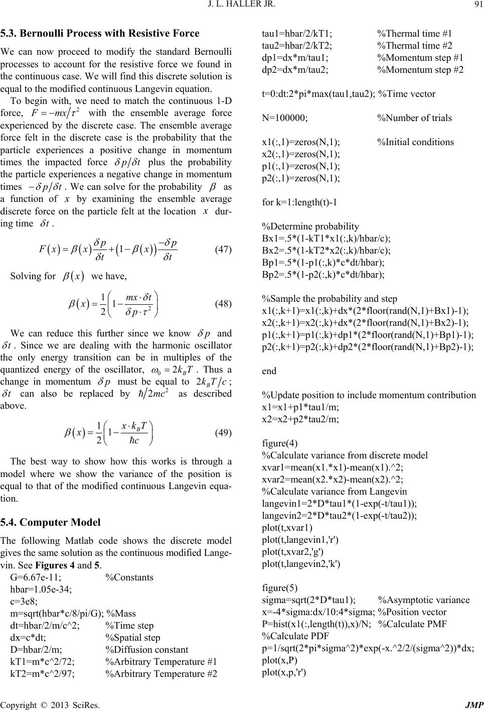

J. L. HALLER JR. 91
5.3. Bernoulli Process with Resistive Force
We can now proceed to modify the standard Bernoulli
processes to account for the resistive force we found in
the continuous case. We will find this discrete solution is
equal to the modified continuous Langevin equation.
To begin with, we need to match the continuous 1-D
force, 2
Fmx

 with the ensemble average force
experienced by the discrete case. The ensemble average
force felt in the discrete case is the probability that the
particle experiences a positive change in momentum
times the impacted force pt

 plus the probability
the particle experiences a negative change in momentum
times pt

 . We can solve for the probability

as
a function of
x
by examining the ensemble average
discrete force on the particle felt at the location
x
dur-
ing time t

.
  
1Fxxpp x
tt








 (47)
Solving for
x

we have,

2
1mx t
p
1
2
x




 




p
(48)
We can reduce this further since we know

and
t

. Since we are dealing with the harmonic oscillator
the only energy transition can be in multiples of the
quantized energy of the oscillator, 0B 2kT

. Thus a
change in momentum p

must be equal to 2kTc
tB;

can also be replaced by 2
2mc as described
above.

1
21B
x
kT
c






x 
(49)
The best way to show how this works is through a
model where we show the variance of the position is
equal to that of the modified continuous Langevin equa-
tion.
5.4. Computer Model
The following Matlab code shows the discrete model
gives the same solution as the continuous modified Lange-
vin. See Figures 4 and 5.
G=6.67e-11; %Constants
hbar=1.05e-34;
c=3e8;
m=sqrt(hbar*c/8/pi/G); %Mass
dt=hbar/2/m/c^2; %Time step
dx=c*dt; %Spatial step
D=hbar/2/m; %Diffusion constant
kT1=m*c^2/72; %Arbitrary Temperature #1
kT2=m*c^2/97; %Arbitrary Temperature #2
tau1=hbar/2/kT1; %Thermal time #1
tau2=hbar/2/kT2; %Thermal time #2
dp1=dx*m/tau1; %Momentum step #1
dp2=dx*m/tau2; %Momentum step #2
t=0:dt:2*pi*max(tau1,tau2); %Time vector
N=100000; %Number of trials
x1(:,1)=zeros(N,1); %Initial conditions
x2(:,1)=zeros(N,1);
p1(:,1)=zeros(N,1);
p2(:,1)=zeros(N,1);
for k=1:length(t)-1
%Determine probability
Bx1=.5*(1-kT1*x1(:,k)/hbar/c);
Bx2=.5*(1-kT2*x2(:,k)/hbar/c);
Bp1=.5*(1-p1(:,k)*c*dt/hbar);
Bp2=.5*(1-p2(:,k)*c*dt/hbar);
%Sample the probability and step
x1(:,k+1)=x1(:,k)+dx*(2*floor(rand(N,1)+Bx1)-1);
x2(:,k+1)=x2(:,k)+dx*(2*floor(rand(N,1)+Bx2)-1);
p1(:,k+1)=p1(:,k)+dp1*(2*floor(rand(N,1)+Bp1)-1);
p2(:,k+1)=p2(:,k)+dp2*(2*floor(rand(N,1)+Bp2)-1);
end
%Update position to include momentum contribution
x1=x1+p1*tau1/m;
x2=x2+p2*tau2/m;
figure(4)
%Calculate variance from discrete model
xvar1=mean(x1.*x1)-mean(x1).^2;
xvar2=mean(x2.*x2)-mean(x2).^2;
%Calculate variance from Langevin
langevin1=2*D*tau1*(1-exp(-t/tau1));
langevin2=2*D*tau2*(1-exp(-t/tau2));
plot(t,xvar1)
plot(t,langevin1,'r')
plot(t,xvar2,'g')
plot(t,langevin2,'k')
figure(5)
sigma=sqrt(2*D*tau1); %Asymptotic variance
x=-4*sigma:dx/10:4*sigma; %Position vector
P=hist(x1(:,length(t)),x)/N; %Calculate PMF
%Calculate PDF
p=1/sqrt(2*pi*sigma^2)*exp(-x.^2/2/(sigma^2))*dx;
plot(x,P)
plot(x,p,'r')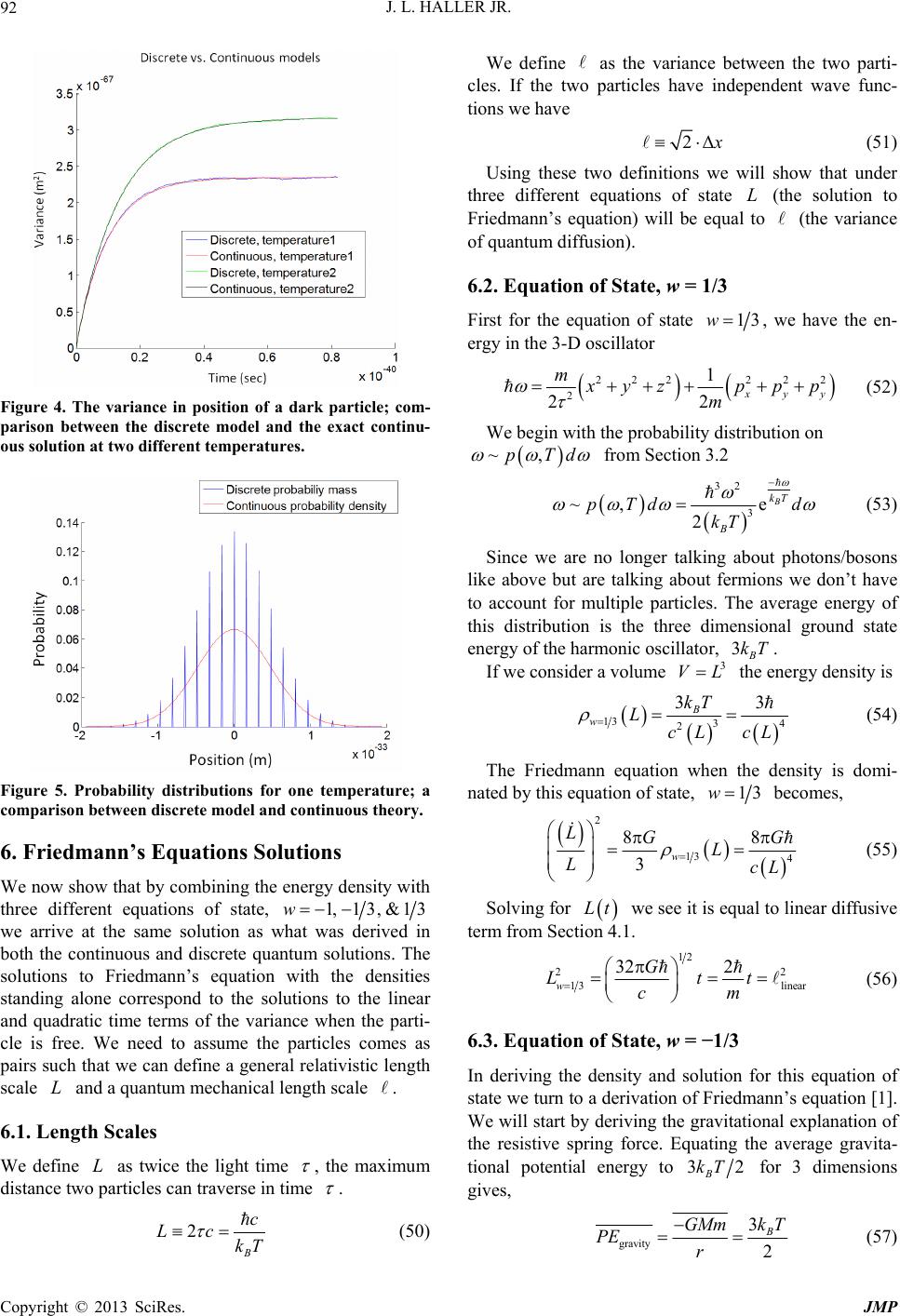

J. L. HALLER JR. 92
Figure 4. The variance in position of a dark particle; com-
parison between the discrete model and the exact continu-
ous solution at two different temperatures.
Figure 5. Probability distributions for one temperature; a
comparison between discrete model and continuous theory.
6. Friedmann’s Equations Solutions
We now show that by combining the energy density with
three different equations of state, 1,13,&13w
we arrive at the same solution as what was derived in
both the continuous and discrete quantum solutions. The
solutions to Friedmann’s equation with the densities
standing alone correspond to the solutions to the linear
and quadratic time terms of the variance when the parti-
cle is free. We need to assume the particles comes as
pairs such that we can define a general relativistic length
scale
L
and a quantum mechanical length scale .

6.1. Length Scales
We define
L
as twice the light time

, the maximum
distance two particles can traverse in time

.
2
B
c
Lc
kT
 


(50)
We define as the variance between the two parti-
cles. If the two particles have independent wave func-
tions we have
2Δ
x
(51)


Using these two definitions we will show that under
three different equations of state
L
(the solution to
Friedmann’s equation) will be equal to (the variance
of quantum diffusion).

6.2. Equation of State, w = 1/3
First for the equation of state 13w, we have the en-
ergy in the 3-D oscillator

2222 2 2
2
1
2 2
x
yy
m
x
yz ppp
m
  (52)
We begin with the probability distribution on


~,pTd


 
from Section 3.2
32
3
~, e
2
B
kT
B
pTd d
kT







3kT
3
VL

(53)
Since we are no longer talking about photons/bosons
like above but are talking about fermions we don’t have
to account for multiple particles. The average energy of
this distribution is the three dimensional ground state
energy of the harmonic oscillator, .
B
If we consider a volume the energy density is
  
13 34
2
33
B
wkT
LcL cL 

 (54)
The Friedmann equation when the density is domi-
nated by this equation of state, 13w

becomes,
 
2
13 4
88
3w
LGG
L
LcL


 




 (55)


L
Solving for t we see it is equal to linear diffusive
term from Section 4.1.
12
22
13 linear
32 2
wG
Ltt
cm







 (56)
6.3. Equation of State, w = −1/3
In deriving the density and solution for this equation of
state we turn to a derivation of Friedmann’s equation [1].
We will start by deriving the gravitational explanation of
the resistive spring force. Equating the average gravita-
tional potential energy to 3 for 3 dimensions
gives,
2
B
kT
gravity
3
2
B
kT
GMm
PE r

 (57)

J. L. HALLER JR. 93
When 3
43Mr


2
4
3
GMmG mr
r
 
 (58)
Due to symmetry we can re-write 2 r as

2
0
3Δ2 34
B
x
mk T [9] to arrive at,

2
2
2
8
3
B
kT
G    (59)
Plugging this back into the relationship between po-
tential energy and force [9] and with time constant
2B kT

 we have,

2
2
22
dd d4
ddd 3
4
8
3
r
B
GMmGmr
FPE
rrrr
mkT
Gmr mr
r




 

 






 

(60)
When a particle moves within the space curved by the
black hole, a resistive spring force is in play. Here we see
a gravitational explanation for the spring force.
Going back to solve for the density we have,
2
0
3
32
B
kT r
T
4Gm   (61)
Where 0 is constant. With

2
22
3Δ32rx
0
and m the reduced Planck mass, the density is
 
0
2
6B mk T
c



13w

  (62)
Friedmann’s equation and its solution show 13 is
equal to the quadratic diffusive term from Section 4.1.
w
L

 
2
13
8
3w
LG
L


 





0
2
2B kT
LmL

 (63)
2
1 3
2B
w
kT
L
m






22
quadratic
t   (64)
Notice the solution of 13w is imaginary because of
the positive curvature associated with this equation of
state [1]. Yet we still have
L
L
cle
. In the next two
paragraphs we derive the holistic energy density,
dark parti

which is always positive and thus
is real.
dark particle
L
1w
The last term we need is a constant energy density,
. To solve for the constant density, we insert
00B (which we show is the asymptotic
value of the solution) into the density of the oscillator.
LmkT



2
2
0
43
3B mkT
c


11 3 0
0
3
ww
LL cL 
 

 (65)
The solution to Friedmann’s equation with this density
is exponentially increasing, however if we add this den-
sity term to our other two densities we see the solution is
equal to the solution of the Langevin equation.
dark partilce11313ww w


 


(66)

   
2
2
2
0
0
422
2
3B
B
DP
mkT
mk T
LcLt Lt 








(67)
By applying calculus, the solution to Friedmann’s
equation with this density is

22
0
2
8
3
B
DP
LkT
GL
LmL

 



 


 (68)

0
2
2 2
0
1e B
kTt
DP B
Lmk T



 (69)


0B0
2kT With



and the
D
2m
L, this is re-written, showing DP equal to the stationary Lange-
vin equation from Section 4.3.


0
22
0 Langevin
41e
t
DP
LD



 (70)
We see the solutions to Friedmann’s equation and the
equations of quantum diffusion behave in the same way.
It is interesting to note that the density vanishes at the
asymptotic value


0DP so we don’t have to
worry about this fermionic density contributing to the
cosmological constant.
0L  
1w
7. Discussion
A similarity one might find with other current work
would be Primordial Black Hole Remnants (PBHR).
Chen uses PBHRs nicely to explain dark matter [23]. In-
terpreted here the density of state is determined by how
the density scales as a function of the length scale. We
have suggested that when the dark particles cannot cou-
ple to ordinary matter the temperature and thus density is
frozen, implying a density of state of and ex-
plaining dark energy. However if the dark particles are
near neutral hydrogen atoms (et al. near galaxies), al-
lowing them to couple and release heat, the density of
state could be positive and the acceleration equation
would be positive, more in line with dark matter [1].
A test of the hypothesis that if neutral hydrogen atoms
are near, dark particles act like more like dark matter
than dark energy would be to look for cosmological ob-
servations where we observe either bountiful or scanty
amount of neutral hydrogen. Perhaps Virgo21 (where we
observe neutral hydrogen atoms and possibly a high den-
sity of dark matter) [24] or global clusters (where any
neutral atoms would be ionized and almost no dark mat-

J. L. HALLER JR. 94
ter) [25] could serve as a first validation.
A further validation of this hypothesis might be ex-
perimentally possible on Earth. A team led by Perl [26]
has suggested two identical side-by-side atom interfer-
ometers could reveal a dark energy density by measuring
the time it takes for atoms to fall through gravity, respec-
tively between the two interferometers. One could build
on this approach and artificially alter the density of the
dark particles by surrounding each interferometer in a
bath of neutral hydrogen atoms (or other suitable sink
that is not dangerous at high temperatures). One bath
could be kept at a low temperature and the other at a high
temperature. If the bath was large enough to allow the
neutral hydrogen and the dark particles to couple and
exchange heat before the dark energy reference frame
moves past the interferometers [26], the density of dark
particles that interacts with the falling atoms would be
different between the hot and the cold interferometers
and the difference would be measured.
Questions still remain, like the exact mechanism for
how the dark particle exchanges heat, and more analysis
is needed for dark particles fully to answer the questions
of dark energy [2,5], or for that matter other open ques-
tions like dark matter [27]. Yet this initial brief report is
intended to set the physical parameters and give guidance
for how the forces of gravity and quantum mechanics
work together and have complementary solutions in a
simple straightforward way.
While it is not possible to create a particle with the
reduced Planck mass artificially, it would explain why
prior experiments have been unable to locate the missing
energy.
As a note, the dark particle was built out of research in
Finite Difference Time Domain (FDTD) modeling of
diffusive motion [19]. By noticing a connection between
Bernoulli’s process [17,21] and black-body radiation [17]
it was possible to derive the continuous version of the
theory. Application to Friedmann’s equation followed a
need to explain the resistive spring force that keeps the
particle stationary. When the theory suggested a density
of black-body radiation was hidden (because the cross
section of the dark particle is on the order of the Planck
length) the tie to dark energy was made.
Mountain View, CA, March 2011.
8. Acknowledgements
JLH would like to thanks his family who encouraged him
to stick with his work. JLH also would like to call out
those around the world who helped, specifically in the
Electrical Engineering and Physics departments at Prince-
ton and Stanford where the foundation of this research
was built.
REFERENCES
[1] A. Liddle, “An Introduction to Modern Cosmology,” 2nd
Edition, John Wiley & Sons, Ltd., W. Sussex, 2003.
[2] P. Peebles and B. Ratra, Reviews of Modern Physics, Vol.
75, 2003, pp. 559-606. doi:10.1103/RevModPhys.75.559
[3] D. Larson, J. Dunkley, et al., “Seven-Year Wilkinson Mi-
crowave Anisotropy Probe (WMAP) Observations: Power
Spectra and WMAP-Derived Parameters,” 2010.
arXiv:1001.4635v2
[4] S. E. Rugh and H. Zinkernagel, Studies in History and
Philosophy of Modern Physics, Vol. 33, 2002, pp. 663-
705. doi:10.1016/S1355-2198(02)00033-3
[5] B. Greene, “The Fabric of the Cosmos,” Vintage Books,
New York, 2004.
[6] L. Papantonopoulos, “Lecture Notes in Physics 720 The
Invisible Universe: Dark Matter and Dark Energy,” Sprin-
ger, Berlin, 2007. doi:10.1007/978-3-540-71013-4
[7] L. Amendola and S. Tsujikawa, “Dark Energy: Theory
and Observations,” Cambridge University Press, Cam-
bridge, 2010. doi:10.1017/CBO9780511750823
[8] S. W. Hawking, Communications in Mathematical Phys-
ics, Vol. 43, 1975, pp. 199-220. doi:10.1007/BF02345020
[9] Feynman, “Lectures on Physics,” Addison-Wesley Pub-
lishing, Reading, 1965.
[10] C. W. Gardiner and P. Zoller, “Quantum Noise,” Springer,
Berlin, 2004.
[11] C. Barcelo, S. Liberati, S. Sonego and M. Visser, Physi-
cal Review D, 83, 2011, Article ID: 041501.
doi:10.1103/PhysRevD.83.041501
[12] S. A. Hayward, Classical and Quantum Gravity, Vol. 15,
1998, p. 3147. doi:10.1088/0264-9381/15/10/017
[13] R. Barkana and A. Loeb, Physics Reports, Vol. 349, 2001,
pp. 125-238. doi:10.1016/S0370-1573(01)00019-9
[14] A. R. Liddle and D. H. Lyth, “Cosmological Inflation and
Large-Scale Structure,” Cambridge University Press, Cam-
bridge, 2000. doi:10.1017/CBO9781139175180
[15] D. F. Walls and G. J. Milburn, “Quantum Optics,”
Springer, Berlin, 1994.
[16] J. Pan, “Email Correspondence,” Fudan University, Shang-
hai, 2007.
[17] Reif, “Fundamentals of Statistical and Thermal Physics,”
McGraw Hill, Boston, 1965.
[18] R. Kubo, Reports on Progress in Physics, Vol. 29, 1966,
p. 255. doi:10.1088/0034-4885/29/1/306
[19] Forsythe & Wasow, “Finite-Difference Methods for Par-
tial Differential Equations,” John Wiley & Sons, Inc.,
New York, 1960.
[20] M. Mecklenburg and B. C. Regan, Physical Review Let-
ters, Vol. 106, 2011, Article ID: 116803.
doi:10.1103/PhysRevLett.106.116803
[21] Chandrasakhar, Reviews of Modern Physics, Vol. 15,
1943.
[22] P. A. M. Dirac, “The Principles of Quantum Mechanics,”
4th Edition, Oxford University Press, Oxford, 1958, p.
262.

J. L. HALLER JR. 95
[23] P. Chen, “Generalized Uncertainty Principle and Dark
Matter,” Quantum Aspects of Beam Physics, World Sci-
entific Publishing, Singapore, 2004, p. 315.
[24] R. Minchin, et al., Astrophysics Journal, Vol. 670, 2007,
pp. 1056-1064. doi:10.1086/520620
[25] S. Mashchenko and A. Sills, Astrophysical Journal, Vol.
619, 2005, pp. 243-257. doi:10.1086/426132
[26] R. J. Adler, H. Mueller and M. L. Perl, “A Terrestrial
Search for Dark Contents of the Vacuum, Such as Dark
Energy, Using Atom Interferometry,” 2011.
arXiv:1101.5626v1
[27] Bertone & Silk, “Particle Dark Matter: Observations,
Models, and Searches,” Cambridge University Press, Cam-
bridge, 2010.